Helioseismology of Pre-Emerging Active Regions II: Average Emergence Properties

Abstract

We report on average sub-surface properties of pre-emerging active regions as compared to areas where no active region emergence was detected. Helioseismic holography is applied to samples of the two populations (pre-emergence and without emergence), each sample having over 100 members, which were selected to minimize systematic bias, as described in Paper I (Leka et al., 2012). We find that there are statistically significant signatures (i.e., difference in the means of more than a few standard errors) in the average subsurface flows and the apparent wave speed that precede the formation of an active region. The measurements here rule out spatially extended flows of more than about 15 m s^-1 in the top 20 Mm below the photosphere over the course of the day preceding the start of visible emergence. These measurements place strong constraints on models of active region formation.

1. Introduction

As discussed in Leka et al. (2012) (Paper I), the mechanisms behind the formation of solar active regions (AR) are not known. Possibilities include magnetic flux tubes rising essentially intact from the base of the convection zone (for a review see Fan, 2009). Alternatively, near-surface effects could dominate the formation mechanism (e.g. Brandenburg, 2005); hybrid scenarios are also a possibility. More generally, understanding of the formation of active regions may lead to a better understanding of the solar dynamo.

Local helioseismology (Gizon & Birch, 2005; Gizon et al., 2010) is among the tools that potentially could be used to determine the subsurface dynamics associated with active region formation. While helioseismic analysis samples the state of the plasma below the visible surface, the interpretation of the results is not always straightforward – especially when the region sampled is quickly changing in context, such as an emerging magnetic flux region.

Numerous studies have attempted to detect – and thus characterize – the signature of one or two active regions at their earliest stages of formation. In one of the earliest studies, Braun (1995) applied Hankel analysis (Braun et al., 1987, 1992) to South Pole observations of the formation of NOAA AR 5247. In the few days before the region’s sunspot was reported, the Hankel analysis detected negative phase shifts (i.e., reduced wave speed). The cause of the phase shifts is not known, and the supporting magnetic measurements were very sparse.

Chang et al. (1999) used acoustic imaging (Chang et al., 1997) applied to MDI and also TON data (Chou et al., 1995) to study the emergence of NOAA AR 7978. Based on an analysis of the focus-depth dependence of observations with a two-day resolution, they suggested that they had detected a magnetic flux concentration moving upwards towards the photosphere. However, the detected positive phase shifts that are co-spatial with the emerging active region are also co-temporal with the appearance of surface flux.

Jensen et al. (2001) used time-distance helioseismology (Duvall et al., 1993) to study two active regions that formed on 11 January 1998 (NOAA AR 8131 and AR 8132) and found changes in the subsurface wave speed that developed at about the same time as the magnetic signatures of the regions were seen in MDI magnetograms. There was no apparent change in subsurface structure before the surface magnetic features were seen.

Hartlep et al. (2011) measured the acoustic power from MDI observations before and during the emergence of AR 10488. This study suggested a decrease in acoustic power in the 3 to 4 mHz band and a reduction in subsurface wavespeed before significant magnetic flux is seen at the photosphere.

Kosovichev (2009) used time-distance helioseismology to study two emerging active regions (NOAA AR 8167 and AR 10488). These case studies inferred increases in the subsurface wave speed associated with flux emergence, however there was no clear indication that these increases preceded the appearance of magnetic flux at the photosphere. Zharkov & Thompson (2008) also used time-distance helioseismology in a case-study of the emergence of NOAA AR 10790; sound-speed increases were also found with (but not prior to) the appearance of surface field.

Komm et al. (2008) used ring-diagram analysis (Hill, 1988) to infer the subsurface flows; it was applied to a few active regions undergoing flux emergence: newly-emerging regions (including AR 10488) were compared to older but resurging active regions. The analysis, which included a comparison with magnetic field in the target areas, found indications of upflows prior to emergence that were followed by downflows.

In an extension of the above study to one of the few truly statistical approaches, Komm et al. (2009, 2011) then used the same ring-diagram analysis approach on a very large sample of active regions characterized by the evolution of the magnetic field (from increasing to decreasing). Key to this study was the “control” dataset of as many “quiet” areas. This study found that growing active regions show a preference for upflows of a fraction of m s^-1, with this effect most apparent at the depth of about 8–10 Mm and reversed below this depth.

There are indications that the details of particular data analysis methods may be very important in determining the helioseismic signals seen for emerging active regions. Ilonidis et al. (2011) showed several cases (including AR 10488) where a travel-time reduction of order 10 s for measurements sensitive to a depth 60 Mm was seen to precede the emergence of an AR. Braun (2012) showed that this result is not reproduced (on the same active regions) using helioseismic holography.

It is difficult to get a consensus picture of the results, likely for a variety of reasons. While most studies report some detection of a signal associated with the appearance of an active region, only Komm et al. (2008), Hartlep et al. (2011), Komm et al. (2009), and Komm et al. (2011) include any comparison to a “control” sample by which to evaluate the detections, although in most cases the criteria for this evaluation are not discussed in detail. The presence of surface fields may complicate the interpretation of any ‘pre-emergence’ signal.

While mention of the surface field evolution was included in most studies, a detailed accounting of the presense (or absence) of surface-field for the full time period used for the helioseismology data analysis was rarely included. The studies cited above are predominantly case studies, with the analysis performed at (or over) varying times in their target regions’ evolution. Case studies are enlightening and critical for guidance – but as discussed in Paper I and shown in Ilonidis et al. (2011), regions emerge with different rates and into different surface contexts; this points to the need for statistical studies, but also reveals why few strong results have emerged from the large-sample studies to date (Komm et al., 2009, 2011).

Numerical simulations have been used to model the emergence of magnetic flux through the last few tens of Mm below the photosphere. Stein et al. (2011) used a radiative magnetoconvection simulation in which horizontal magnetic field was advected into the simulation domain by upflows through the lower boundary (20 Mm below the photosphere). For the case of 10 kG field strength, the magnetic field emerges through the photosphere in about 32 hours. In this case, the field has only a weak effect on the convection and the emergence process is largely controlled by the convection. Cheung et al. (2010), also using a radiative magnetoconvection simulation, studied the emergence of a semi-torus of twisted field. In this case, the magnetic structure was forced through the lower boundary with a vertical velocity of 1 km s^-1 and took about 2 hours to rise to the photosphere from a depth of 7.5 Mm. In these simulations, vertical flows of about 0.5 km s^-1 and diverging horizontal flows of order a few km s^-1 are associated with the flux emergence at the photosphere. These two simulations show scenarios for flux emergence with very different observational implications.

In the present study, we combine a statistically-significant sample and a control group, with a detailed analysis of the surface magnetic field (Paper I), and examine the differences in pre-emergence behavior in an average sense. We undertake a more detailed statistical analysis of the two populations in the next paper in this series (Barnes et al., 2012, Paper III). It should be noted that the analysis used herein (see §3) relies on “raw” travel-time shifts rather than inversions used by most of the studies cited above; as such, we avoid potential complications and uncertainties of the inversions, while sacrificing details about the depth of any perturbations detected. Nonetheless, we show that on average there are statistically significant sub-surface flows and changes in wave speed that precede AR emergence; these results place strong constraints on models of active region formation, even when individual case studies show no clear signature of emergence.

The layout of the paper is as follows. In §2 we review the data sets that are used in the helioseismic measurements. In §3 we detail the application of helioseismic holography to these data sets. A statistical summary of the results is shown in §4. We discuss the main results and outline some possibilities for future work in §5.

2. The Data

The GONG Doppler data cubes for active regions before their emergence (we will refer to these as pre-emergence, or “PE” cases) and for quiet-Sun control cases that are not associated with AR emergence (non-emergence, or “NE”, cases), accompanied by the associated MDI magnetograms are described in detail by Paper I. To briefly review the procedure described there: we selected a sample of 107 pre-emergence cases and the same number of non-emergence cases. These samples of the two populations (PE and NE) were selected to have well-matched distributions in disk location (latitude/CMD) and time (within the solar cycle), to avoid biases in the seismology due to projection and instrumental effects. For the PE cases, a refined emergence time $t_{0}$ was defined as when the change in the total absolute flux (as measured from MDI) reached 10% of the maximum increase detected within a 3-day window of its nominal (NOAA-defined) emergence time. The GONG data cubes were 1664 minutes long (one “GONG-day”), spanning from 1648 minutes before $t_{0}$ to 16 minutes after. These 1664 minute cubes were divided into five time intervals of 384 minutes each, with an overlap of 64 minutes between time intervals. The time between the start of each time interval is 320 minutes. The cadence of the GONG Doppler data is one minute per image.

As described by Paper I, each of the Doppler images is Postel projected (Pearson, 1990) on to a map with a scale of 1.5184 Mm pixel^-1 and a size of 256$\times$256 pixels². Figure 1 shows the mean power spectrum of the NE regions. The ridges in the power spectrum are visible up to about $k=1.5~{}{\rm rad\,Mm}^{-1}$.

Potential field extrapolations from MDI magnetograms are used to estimate the radial component of the magnetic field (for details see Paper I, ). These estimates of the radial magnetic field are then projected into the same map coordinates as the GONG Dopplergrams and averaged over the same time intervals. The result of this procedure is a set of maps of radial magnetic field estimates, one map for each time interval for each PE and NE case.

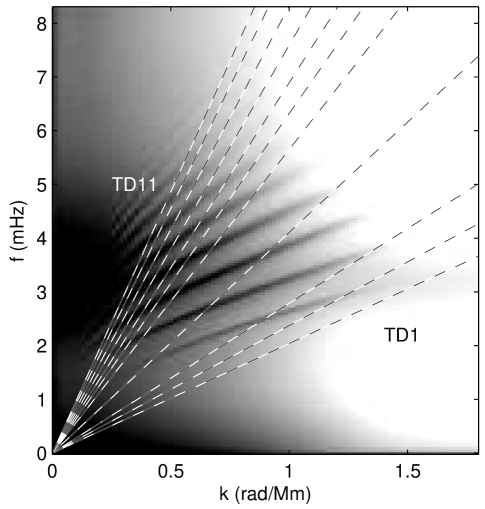
Figure 1.— Mean power spectrum of the GONG Doppler data cubes for all of the NE regions. The ridges are visible up to about horizontal wavenumber $k=1.5~{}{\rm rad\,Mm}^{-1}$. The central phase speeds for the filters used in this work (we use the filters from Couvidat et al., 2005) are shown as dashed lines (filter TD1 has the lowest phase speed and TD11 has the highest). The width of the filters is similar to the distance between filters.

filter	inner radius( Mm)	outer radius (Mm)	depth (Mm)
TD1	3.7	8.7	1.4
TD2	6.2	11.2	2.2
TD3	8.7	14.5	3.2
TD4	14.5	19.4	6.2
TD5	19.4	29.3	9.5
TD6	26.0	35.1	11.4
TD7	31.8	41.7	13.3
TD8	38.4	47.5	15.7
TD9	44.2	54.1	18.2
TD10	50.8	59.9	20.9
TD11	56.6	66.7	23.3

Table 1Table of annulus size and lower turning point depth, taken from Table 1 of Couvidat et al. (2005). The first column shows the filter name. The remaining three columns show the inner annulus radius (Mm), outer annulus radius (Mm), and the lower turning point depth (computed at the central phase speed of each filter).

3. Helioseismic Holography

Helioseismic holography (Lindsey & Braun, 2000) is a tool that uses measurements of solar oscillations to infer subsurface conditions; it is very similar to time-distance helioseismology (Duvall et al., 1993). See Gizon & Birch (2005) for a detailed review of helioseismic holography. Here, we applied surface-focusing helioseismic holography to each of the five time intervals of each of the PE and NE data cubes.

The basic steps in the analysis are: 1) track and Postel project GONG Dopplergrams (described in the previous section), 2) apply phase-speed filters, 3) compute local-control correlations, and 4) measure travel-time shifts. Phase-speed filters (Duvall et al., 1997) isolate waves with particular ranges in lower turning points. We used filters 1 through 11 (here denoted as filters TD1 to TD11) as described in Table 1 from Couvidat et al. (2005). These filters cover the range in sampling depth from about 1.4 Mm (filter TD1) to about 23.3 Mm (filter TD11), as shown in Table 1. Each phase-speed filter leads to a separate filtered data cube (i.e., filtered time series of Dopplergrams). From each of these filtered data cubes, we then computed local-control correlations (e.g., Lindsey & Braun, 2000, these are analogous to time-distance correlations) for both center-annulus and center-quadrant geometries (see e.g., Duvall et al., 1997, for a description of these geometries). The annulus sizes are shown in Table 1 and were taken from Table 1 of Couvidat et al. (2005). Finally, we measured travel-time shifts from the center-annulus and center-quadrant local-control correlations using the phase method of Lindsey & Braun (2000). We emphasize that due to the tracking procedure, most of the effect of solar rotation is removed from the measurements shown here. In addition, as described in §4, we remove smooth fits to all of the maps of travel-time maps. As a result, the travel-time maps shown here do not include large-scale effects (e.g., differential rotation and meridional flow).

Throughout this paper, we use $x$ and $y$ to denote the coordinates in the Postel projection geometry, with $x$ increasing in the direction of rotation and $y$ increasing to the north. We use ${\delta\tau}_{x}$ to denote east-west travel-time differences (i.e., the difference in travel times between east-going and west-going waves) and ${\delta\tau}_{y}$ to denote north-south travel-time differences. These travel-time differences are mostly sensitive to east-west (north-south) flows, with a negative ${\delta\tau}_{x}$ (${\delta\tau}_{y}$) indicative of a flow to the west (north).

Following the usual convention, we denote the outgoing (i.e., center-to-annulus) travel-time shift (shift relative to the average) by ${\delta\tau}_{\rm out}$ and the in-going (i.e., annulus-to-center) travel-time shift by ${\delta\tau}_{\rm in}$. From these we construct the “out minus in” travel-time shift ${\delta\tau}_{\rm oi}={\delta\tau}_{\rm out}-{\delta\tau}_{\rm in}$ and the mean travel-time shift ${\delta\tau}_{\rm mn}=\left[{\delta\tau}_{\rm out}+{\delta\tau}_{\rm in}\right]/2$. The one-way center-annulus travel times ${\delta\tau}_{\rm in}$ and ${\delta\tau}_{\rm out}$ are sensitive to the isotropic wave speed and also to vertical flows and converging/diverging horizontal flows. These two effects (i.e., change in isotropic waves speed and the presence of flows) are approximately separated by ${\delta\tau}_{\rm oi}$, which is sensitive mostly to diverging / converging horizontal flows and vertical flow, and ${\delta\tau}_{\rm mn}$ which is more sensitive to changes in the isotropic wave speed. The sign conventions are such that ${\delta\tau}_{\rm mn}<0$ is interpreted as a signature of increased wave speed, and ${\delta\tau}_{\rm oi}<0$ is the signature of a diverging flow.

From the quantities ${\delta\tau}_{x}$ and ${\delta\tau}_{y}$ we computed proxies for the vertical component of the flow vorticity (denoted vort) ${\rm vor}=\partial_{x}{\delta\tau}_{y}-\partial_{y}{\delta\tau}_{x}$ and for the horizontal flow divergence (denoted div) as ${\rm div}=\partial_{x}{\delta\tau}_{x}+\partial_{y}{\delta\tau}_{y}$. The derivatives were computed in the Fourier (horizontal wavevector) domain.

4. Results

The analysis is presented in three stages: first, individual examples; second, averages over all samples (separately for the two populations) but retaining the spatial information; and third, an analysis of the spatial average over a small central region, and its temporal evolution, again contrasting the averages over the two populations.

4.1. Individual Active Region Examples

Figure 2 shows, for the case of the emergence of AR 9729, the ${\delta\tau}_{\rm mn}$ maps for filter TD5 (lower turning point of about 9.5 Mm) together with estimates of the radial magnetic field obtained from potential field extrapolations (details are in Paper I) from MDI 96-minute magnetograms. In this case, the emergence takes place in a region with strong nearby magnetic fields. These pre-existing surface magnetic fields have corresponding negative features (i.e. increased apparent wave speed) in the maps of ${\delta\tau}_{\rm mn}$. Using the NE cases, we estimate that the noise level in the smoothed maps (for maps with duty cycle of better than 70%) of ${\delta\tau}_{\rm mn}$ for filter TD5 is about 0.9 s. Therefore, many of the weaker features seen in the travel-time shifts in Figure 2 are likely due to noise. With this noise level in mind, there is no apparent evolution with time. Notice that this figure covers roughly the 24 hours before emergence, and as a result the development of the active region is not seen in either the magnetograms or the travel-time maps. This is a typical example of the PE cases.

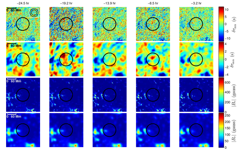
Figure 2.— Example, for NOAA AR 9729, of the time evolution of the ${\delta\tau}_{\rm mn}$ and of the surface magnetic field over the 24 hr prior to the appearance of the region’s emerging magnetic flux. Time advances from left to right in steps of 320 minutes; the mid-interval time relative to $t_{0}$ is labeled at the top. Top row: maps of ${\delta\tau}_{\rm mn}$ for filter TD5 (corresponding to a depth of about 9.5 Mm) for each of the time intervals. The last column covers $-368{\rm min}\leq t_{0}\leq 16{\rm min}$, little if any active-region flux emergence should be visible. Second row: same as the top row after smoothing with a Gaussian with full-width at half maximum (FWHM) of 9.99 pixels (about 15 Mm). Notice the change in color scale; the spatial smoothing reduces the amplitude of the fluctuations in ${\delta\tau}_{\rm mn}$. Third row: the evolution of the unsigned radial magnetic field strength. Fourth row: same, but after the same smoothing as was applied to the maps of ${\delta\tau}_{\rm mn}$; again, the color scale changes because of the reduced amplitude of the fluctuations. Notice that negative travel-time shifts appear co-spatial with the areas of strongest magnetic field. The black circle in all panels shows the averaging region (see § 4.3) surrounding the area where the AR will emerge. The inset (top left panel) indicates the size of the annulus used in the holography measurements for filter TD5. Notice the higher noise level in ${\delta\tau}_{\rm mn}$ maps for the second time interval; this is caused by a low (60%) duty cycle. As discussed in §4.2, such low duty cycle time intervals are excluded in later analysis.

Figure 3 shows another example, this time for the pre-emergence time evolution of NOAA AR 10488, that was also studied by Komm et al. (2008), Kosovichev & Duvall (2008), Kosovichev (2009), Hartlep et al. (2011), and Ilonidis et al. (2011). In our analysis, there is no discernable signal greater than $\pm 2\ {\rm s}$ in the first four time intervals (covering approximately $-27\ {\rm hr}\leq t_{0}\leq-5\ {\rm hr}$) in the raw or smoothed ${\delta\tau}_{\rm mn}$ maps; the raw and smoothed magnetic flux maps are similarly bare. In fact, there are fewer areas of nearby strong field and spatially-associated ${\delta\tau}_{\rm mn}$ signal than in the previous example (Figure 2).

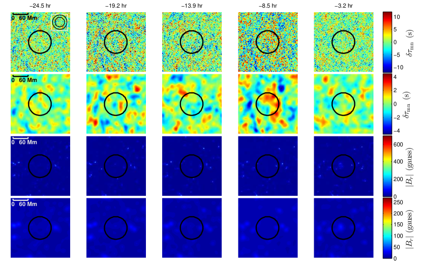
Figure 3.— Same as Figure 2, but for AR 10488. As in Figure 2, notice that the color scale is different for the first and seconds rows, and for the third and fourth rows. In this case, there is no clear signature of emergence in the magnetic field or ${\delta\tau}_{\rm mn}$ maps in the 24 hours before emergence.

In this case, a feature with $\approx 50$ G magnitude appears in the average magnetogram for the last time interval. This is not strictly unusual; the automated definition of emergence time that we have used, while refined earlier by hours or days from the NOAA-assigned emergence time, may still allow magnetic field at the surface prior to the “emergence time” $t_{0}$ of 11:11 UT on 26 October 2003 in this case (see Paper I, for details). Here we note, however, that less objective definitions of emergence lead to less repeatable results; flux emergence does not always follow a standard template for temporal evolution. Nonetheless, the signal is weak in this last time interval (it is an average over $\approx 6$ hr) and has no corresponding features in the maps of ${\delta\tau}_{\rm mn}$, though this may be due mostly to noise (which we expect, based on the statistics of the NE cases, to be about 0.9 s in the smoothed travel-time maps for the filter shown in Fig. 3).

Of the other studies of this region, all use a different emergence time; here, we summarize the results relative to our definition of emergence time. Komm et al. (2008) begin their analysis on 27 October 2003, and thus there is no possibility for a direct comparison of the results, as this is the day following our analysis. Kosovichev & Duvall (2008); Kosovichev (2009) first see wave speed perturbations in data from an 8 hr time interval centered at approximately one hour after $t_{0}$, and describe this as a pre-emergence signature with growth of the magnetic flux starting at approximately $t_{0}+9$ hr. Thus, the results are similar to this study in that no clear subsurface signal appears when only data from at least a few hours prior to $t_{0}$ are used in the analysis.

Hartlep et al. (2011) state that magnetic field starts to appear at the surface approximately 2 hr before $t_{0}$, while significant magnetic flux appears at around $t_{0}$. Their finding of a change in the acoustic power in the 3–4 mHz frequency range, averaged over 128 minutes, centered approximately two hours before $t_{0}$ is likely related to the weak magnetic field seen in the last time interval of this study.

Finally, Ilonidis et al. (2011) report a reduction in the mean travel-time of about 16 s at a depth of about 60 Mm (much deeper than the 9.5 Mm shown here) from an 8 hr data set centered approximately 7.5 hr before $t_{0}$. The difference in the depths considered again makes a direct comparison impossible, but see Braun (2012) for a discussion of using helioseismic holography to examine the same depth range.

Even for this most frequently studied active region emergence, little direct comparison is possible due to different time intervals and depth ranges covered. However, in the most comparable studies of Kosovichev & Duvall (2008) and Kosovichev (2009), the results are similar to the results presented here when the difference in the stated time of emergence is accounted for.

4.2. Averages for the Two Populations

We now present the results of averages over all members of a sample (e.g., the average over all NE cases) with duty cycle greater than 70% (c.f., Paper I, Table 3; all averages in this paper will use this constraint on the duty cycle). Averages taken in this manner are indicated by angle brackets, $\langle\cdot\rangle$. For the travel-time maps, large-scale spatial variations resulting from the Postel projection have been removed prior to averaging, using a second order polynomial fit in the $x$ and $y$ map coordinates (the functional form of the fitting polynomial is $f(x,y)=a_{1}x^{2}+a_{2}y^{2}+a_{3}xy+a_{4}x+a_{5}y+a_{6}$). For this analysis, all maps were smoothed with a Gaussian of FWHM of 9.99 pixels. In the case of the PE samples, the emergence site was not initially at the center of every data cube. To improve the signal/noise ratio for this analysis, we aligned all of the travel-time maps (and magnetograms) before averaging. As described by Paper I, the alignment was done by first computing, for each PE case, the centroid of the pixels where the change in time averaged $B_{r}$ between time interval 0 (about 27 to 21 hours before emergence) and the average of $B_{r}$ computed over the 4 to 10 hours after emergence was more than 30% of the maximum.

Figure 4 shows the time-evolution of ${\langle\delta\tau_{\rm mn}\rangle}$, ${\langle\delta\tau_{x}\rangle}$, and ${\langle\delta\tau_{y}\rangle}$ maps over all of the NE cases, for filter TD5. Also shown is the evolution of the corresponding average of the unsigned radial magnetic field. The average magnetic field is overall weak and unchanging over these averages. There are regions where the average magnetic field is above 20 Gauss, generally near the edges of the map. Nearby plage field was permitted in the definition of a “non-emerging” region (see Paper I, for a discussion). The maps of ${\langle\delta\tau_{\rm mn}\rangle}$, ${\langle\delta\tau_{x}\rangle}$, and ${\langle\delta\tau_{y}\rangle}$, all for filter TD5, show no features stronger than $\pm 1{\rm s}$, and little spatial or temporal coherence between the time intervals.

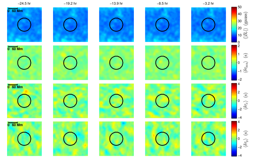
Figure 4.— Evolution (left to right, times labeled as Figure 2) of $\langle|B_{r}|\rangle$, ${\langle\delta\tau_{\rm mn}\rangle}$,${\langle\delta\tau_{x}\rangle}$, and ${\langle\delta\tau_{y}\rangle}$ maps for filter TD5, of the average for each time interval taken over all NE samples with duty cycle great than 70%. No clear and persistent features are visible, and no features are present that are distinctly greater than the noise. The black circle in each panel indicates the area that is spatially averaged in subsequent analysis.

Figure 5 shows the time-evolution of the same averaged quantities for the PE samples (spatially co-aligned as described above). The difference between these results and those shown in Figure 4 is striking. There is a persistent feature of order -1 s in the maps of ${\langle\delta\tau_{\rm mn}\rangle}$ for filter TD5, with the strength of the signal increasing as $t_{0}$ approaches. This signal appears to be associated with a feature in the average magnetogram in the same location. In general, we see correspondence between strong features in the average radial magnetic field strength and features in the mean travel-time shifts. One possibility is that the surface magnetic field is the direct cause of the travel-time shift (i.e., the showerglass effect of Lindsey & Braun, 2005). We undertake a statistical study of this possibility in the next paper in this series (Barnes et al., 2012, Paper III).

We also see (Fig. 5) that the average radial field strength at the emergence site also increases as $t_{0}$ approaches. While the definition of $t_{0}$ allows nearby flux to be present prior to $t_{0}$, and may be uncertain to a few hours (see Paper I), a signal can be seen at least a day before emergence. There is a clear preference for surface field to be located at the emergence site prior to significant flux emergence (see Paper I and Paper III for further discussion).

Figure 5 also shows there are persistent features in the maps of ${\langle\delta\tau_{x}\rangle}$ and ${\langle\delta\tau_{y}\rangle}$ with amplitudes of about 2 s beginning a day prior to $t_{0}$. For the first four time intervals, there are hints of anti-symmetric features in these maps; a flow converging towards the emergence site at approximately 15 m s^-1 might give such a distribution of travel times. The maps for the last time interval are more complicated; in particular the map of ${\langle\delta\tau_{x}\rangle}$ shows what might possibly be the signal of the magnetic region moving in the prograde direction (e.g., Zhao et al., 2004).

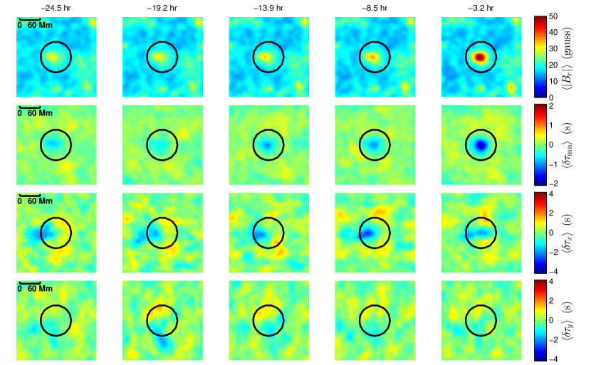
Figure 5.— Same as Figure 4, showing (top: bottom) $\langle|B_{r}|\rangle$, $\langle{\delta\tau}_{\rm mn}\rangle$, $\langle{\delta\tau}_{x}\rangle$, and $\langle{\delta\tau}_{y}\rangle$ but for the average over all of the PE samples (with duty cycle great than 70%) again for filter TD5. The features in the maps of ${\langle\delta\tau_{\rm mn}\rangle}$ are spatially correlated with those in the maps of $\langle|B_{r}|\rangle$. For the first four time intervals, there are anti-symmetric features in the travel-time differences ${\langle\delta\tau_{x}\rangle}$ and ${\langle\delta\tau_{y}\rangle}$; these features might be hints of a converging flow. The map of ${\langle\delta\tau_{x}\rangle}$ for the last time intervals shows what might be evidence of a weak prograde flow associated with the surface magnetic field (e.g. Zhao et al., 2004). These travel-time differences are of order two seconds, which for filter TD5 corresponds to a flow of about 15 m  s^-1.

4.3. Spatial Averages for the Two Populations

Motivated by Figure 5, and to focus more closely on the site of flux emergence, we next present spatial averages. The averages are computed, for each sample in the PE and NE populations, over disks of radius 45.5 Mm centered on the emergence location (as defined using the centroid mentioned above, c.f. details in Paper I), and indicated in Figures 2–5. We denote these initial spatial averages with an over-bar, e.g., $\overline{\delta\tau_{x}}$. As discussed earlier, data cubes with duty cycle less than 70% are omitted from this analysis (c.f., Paper I, Table 3). We then compute averages over the entire PE and NE samples, separately for each time interval, and the standard error in the mean ($\sigma/\sqrt{n}$, where $\sigma$ is the standard deviation and $n$ is the number of samples included). The results, described further below, are depicted in a multi-panel presentation that includes the parameters, all filters, and the temporal evolution of both PE and NE averages and their errors within each filter/parameter combination.

Figure 6 shows the time evolution of ${\langle\overline{\delta\tau_{\rm mn}}\rangle}$, ${\langle\overline{\delta\tau_{x}}\rangle}$, and ${\langle\overline{\delta\tau_{y}}\rangle}$. The figure also shows ${\langle\overline{\delta\tau_{x}\cos{\theta}}\rangle}$ and ${\langle\overline{\delta\tau_{y}\sin{\theta}}\rangle}$; these quantities are the sample average (angle brackets) of the spatial averages (over-bar) of either ${\delta\tau}_{x}$ weighted by $\cos{\theta}$ or ${\delta\tau}_{y}$ by $\sin{\theta}$, where $\theta$ is the angle measured counter-clockwise from the direction of solar rotation (the $+\hat{\bf x}$ direction).

Focusing first on the measurements ${\langle\overline{\delta\tau_{\rm mn}}\rangle}$, there appear to be clear and sustained differences between the PE and NE cases for all but the shallowest filters (TD1, TD2, and TD3), and the deepest filter (TD11). The sense of the difference is generally that ${\langle\overline{\delta\tau_{\rm mn}}\rangle}$ is more negative for the PE cases than the NE cases. The NE cases are very temporally consistent between filters, and in most filters the difference between the NE and PE samples increases as time approaches the emergence time $t_{0}$, with the PE population results increasing in (negative) magnitude. The amplitude of this effect is of order tenths of a second. This may perhaps be a consequence of the surface magnetic field and is discussed in detail by Paper III.

Regarding the flow measurements ${\langle\overline{\delta\tau_{x}}\rangle}$ and ${\langle\overline{\delta\tau_{y}}\rangle}$, there is no clear difference between the NE and PE populations. The anti-symmetric averages ${\langle\overline{\delta\tau_{x}\cos{\theta}}\rangle}$ and ${\langle\overline{\delta\tau_{y}\sin{\theta}}\rangle}$, however, show substantial differences (e.g. of between two and three standard errors for filter TD3) for filters TD2-TD5 (depths of 2.2 Mm to 9.5 Mm). These differences are due to the anti-symmetric features seen in Figure 5. Notice that in all of these filters (TD2-TD5) these features are seen even at 24 hours before emergence.

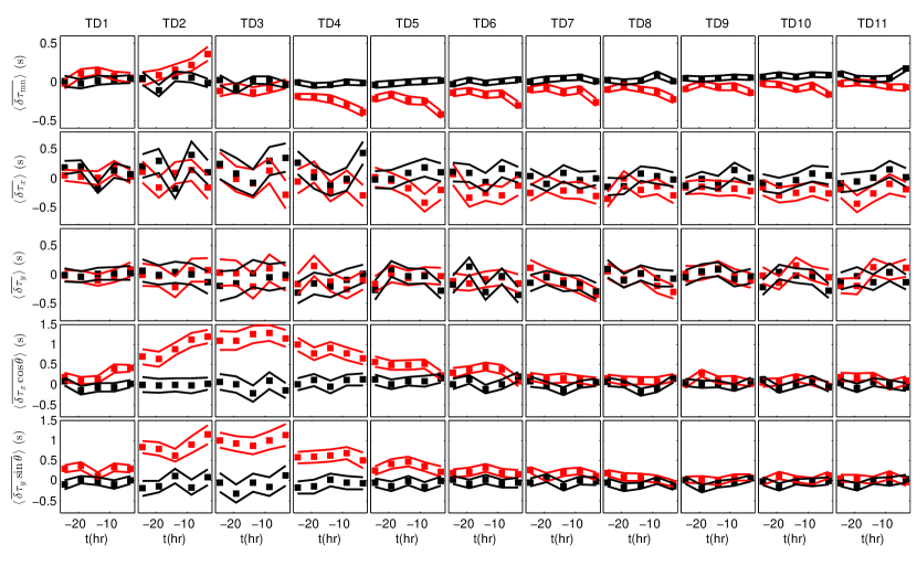
Figure 6.— Summary presentation of (top:bottom) ${\langle\overline{\delta\tau_{\rm mn}}\rangle}$, ${\langle\overline{\delta\tau_{x}}\rangle}$, ${\langle\overline{\delta\tau_{y}}\rangle}$, ${\langle\overline{\delta\tau_{x}\cos{\theta}}\rangle}$, and ${\langle\overline{\delta\tau_{y}\sin{\theta}}\rangle}$ (see text for description); shown are the average results for both PE (red) and NE (black) spatial averages, as a function of time (x-axis). Each column (left:right) corresponds to a different phase-speed filter, with depth of the lower turning point increasing from left to right (see Table 1). The range surrounding each point indicates the associated errors. These results are discussed in the text.

Figure 7 shows the time evolution of ${\langle\overline{\delta\tau_{\rm in}}\rangle}$, ${\langle\overline{\delta\tau_{\rm out}}\rangle}$, ${\langle\overline{\delta\tau_{\rm oi}}\rangle}$, $\langle\overline{\rm div}\rangle$, and $\langle\overline{\rm vor}\rangle$. The parameters ${\langle\overline{\delta\tau_{\rm in}}\rangle}$ and ${\langle\overline{\delta\tau_{\rm out}}\rangle}$ show fairly consistent differences between the PE and NE samples. These appear to be roughly consistent with the change in ${\langle\overline{\delta\tau_{\rm mn}}\rangle}$ seen in Figure 6. Similarly, there is a trend that ${\langle\overline{\delta\tau_{\rm oi}}\rangle}$ is systematically larger in the PE than the NE cases, again this is qualitatively consistent with the maps of ${\langle\delta\tau_{x}\rangle}$ and ${\langle\delta\tau_{y}\rangle}$ from Figure 5.

Other results are less pronounced. For example, in $\langle\overline{\rm div}\rangle$ there is a weak difference between the NE and PE samples for filters TD4, TD5, and TD6; the sign is consistant with a converging flow. Other PE/NE differences are either fleeting or at the one-$\sigma$ level. For example, the average divergence $\langle\overline{\rm div}\rangle$ shows a strong positive feature for filter TD1 in the second time interval, this feature is not persistent in time and may be noise. In the first time interval, there are differences, at the one-$\sigma$ level, between the $\langle\overline{\rm vor}\rangle$ for the PE and NE cases for filters TD2, TD3, TD5, and TD11. There are also one-$\sigma$ differences for the last time interval for filter TD2, the second time interval for TD7, and the last time interval for TD9.

In the interest of recognizing spurious results, we note the following. Assuming that the variances of two distributions are equal (e.g., PE and NE; the assumption is reasonable if the variance is predominantly due to noise), simply by chance alone approximately 16% of the results should have the difference between the means greater than the sum of the standard errors (i.e., $|\bar{x}_{1}-\bar{x}_{2}|>\sigma_{1}/\sqrt{n_{1}}+\sigma_{2}/\sqrt{n_{2}}$, where $\sigma$ is the standard deviation, and as mentioned above, $\sigma/\sqrt{n}$ is the standard error shown in Figures 6 and 7). This translates to roughly nine $1-\sigma$ results per parameter that are expected to be purely spurious. For the difference being twice the sum of the standard errors, the expectation shrinks to 0.5%, or less than one result per parameter, and for the difference being three times the sum, the expectation would be a nearly negligible $3\times 10^{-3}$%. For the case of $\langle\overline{\rm vor}\rangle$, there are seven such points. Hence, it seems possible that the differences we have seen in $\langle\overline{\rm vor}\rangle$ and $\langle\overline{\rm div}\rangle$ as well as some of the other differences between the PE/NE samples are simply the result of noise. Conversely, the many large differences in ${\langle\overline{\delta\tau_{\rm in}}\rangle}$, for example, are very likely real.

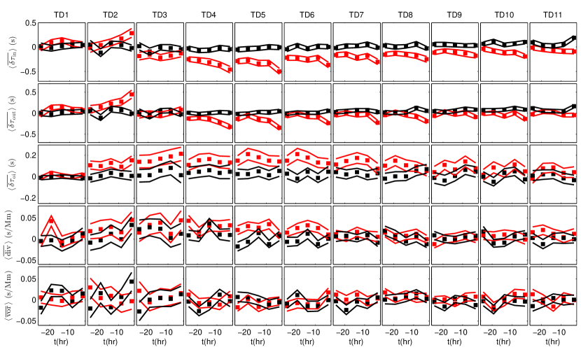
Figure 7.— Temporal evolution of ${\langle\overline{\delta\tau_{\rm in}}\rangle}$, ${\langle\overline{\delta\tau_{\rm out}}\rangle}$, ${\langle\overline{\delta\tau_{\rm oi}}\rangle}$, $\langle\overline{\rm div}\rangle$, and $\langle\overline{\rm vor}\rangle$ for the PE (red) and NE (black) populations. The layout of the figure is the same as for Figure 6.

4.4. Results for the “Ultra-Clean” Pre-Emergence Sample

In Paper I we describe a subset of the PE sample which we deemed “ultra-clean”. These 11 hand-selected emerging active regions all eventually reached a size of at least 70 $\mu\!\!$ H and displayed a monotonically increasing flux history after a distinct and unambiguous emergence time $t_{0}$, appearing into an otherwise weak field area.

Figure 8 shows $\langle|B_{r}|\rangle$, ${\langle\delta\tau_{\rm mn}\rangle}$, ${\langle\delta\tau_{x}\rangle}$, and ${\langle\delta\tau_{y}\rangle}$ averaged over this subsample of the PE cases. As in the average over all PE cases, the strongest magnetic feature appears at the emergence site in the last time interval. Also as in the average of all PE cases, there is an apparently associated feature in the average of ${\delta\tau}_{\rm mn}$. Interestingly, a similar feature in the -13.9 hr interval has no corresponding feature in $\langle|B_{r}|\rangle$, and there is no ${\langle\delta\tau_{\rm mn}\rangle}$ feature in the interim -8.5 hr interval. Due to the smaller number of regions, the noise is higher in these averages (we expect the noise to be about $0.9/\sqrt{10}\approx 0.3$ s in the smoothed maps of ${\langle\delta\tau_{\rm mn}\rangle}$), thus, it is not clear if lack of features in the average ${\delta\tau}_{\rm mn}$ map at the earlier times is significant. The ${\langle\delta\tau_{x}\rangle}$ and ${\langle\delta\tau_{y}\rangle}$ maps are also noisier than the corresponding maps in Figure 5, as expected. There is still a weak suggestion in some of the time intervals of anti-symmetric features in the average maps of ${\delta\tau}_{x}$ and ${\delta\tau}_{y}$ (again as in Fig. 5). Still, it is worth emphasizing that these 11 hand-picked regions presumably represent the best-case (i.e. relatively simple emergence into quiet Sun) scenario for detecting helioseismic signals in the day prior to an active region’s emergence.

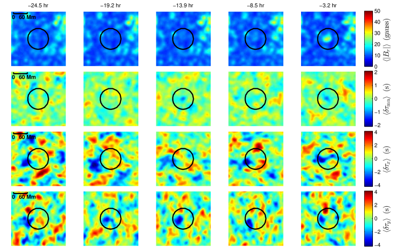
Figure 8.— Same as Figure 4, but for an average over the eleven hand-selected “ultra-clean” PE regions. In this case, the $\langle|B_{r}|\rangle<20~{}{\rm G}$ at the emergence site until the last time interval. The noise level is higher in the ${\langle\delta\tau_{\rm mn}\rangle}$, ${\langle\delta\tau_{x}\rangle}$, and ${\langle\delta\tau_{y}\rangle}$ compared with the averages shown in Figure 5, as the average is over a much smaller sample of regions (roughly nine instead of ninety, see Table 3 of Paper I). There is a very weak signal in ${\langle\delta\tau_{\rm mn}\rangle}$ at the time intervals centered at -13.9 hr and -3.2 hr.

Figure 9 shows the spatial and ensemble averages ${\langle\overline{\delta\tau_{\rm mn}}\rangle}$, ${\langle\overline{\delta\tau_{x}}\rangle}$, ${\langle\overline{\delta\tau_{y}}\rangle}$, ${\langle\overline{\delta\tau_{x}\cos{\theta}}\rangle}$, ${\langle\overline{\delta\tau_{y}\sin{\theta}}\rangle}$ for the subsample of eleven PE regions, along with the same average over the NE regions shown in Figure 6. The results are less clear than what is presented in Figure 6, due to the much smaller sample size for the PE population (about nine instead of 90, after accounting for time-intervals with low duty cycle, see Table 3 of Paper I). For this subsample of pre-emergence active regions, no difference between the ${\langle\overline{\delta\tau_{\rm mn}}\rangle}$ is seen. This may be because in the hand-selected subsample of PE cases, there is very little nearby surface magnetic field except in the last time interval (see Fig. 8). There is no apparent signal in ${\langle\overline{\delta\tau_{x}}\rangle}$ or ${\langle\overline{\delta\tau_{y}}\rangle}$. The differences between the PE and NE populations can, however, still be seen in the anti-symmetric averages ${\langle\overline{\delta\tau_{x}\cos{\theta}}\rangle}$, ${\langle\overline{\delta\tau_{y}\sin{\theta}}\rangle}$ for filters TD2-TD5. It is noteworthy that these differences remain, even when the differences in ${\langle\overline{\delta\tau_{\rm mn}}\rangle}$ are not visible. This suggests that there are different physical mechanisms responsible for these two effects.

Figure 10 shows the spatial and ensemble averages ${\langle\overline{\delta\tau_{\rm in}}\rangle}$, ${\langle\overline{\delta\tau_{\rm out}}\rangle}$, ${\langle\overline{\delta\tau_{\rm oi}}\rangle}$, $\langle\overline{\rm div}\rangle$, and $\langle\overline{\rm vor}\rangle$ for the subset of eleven PE regions, following Figure 7. For the variables ${\langle\overline{\delta\tau_{\rm in}}\rangle}$, ${\langle\overline{\delta\tau_{\rm out}}\rangle}$, ${\langle\overline{\delta\tau_{\rm oi}}\rangle}$, and $\langle\overline{\rm div}\rangle$ there are no statistically significant differences in the means for the two populations. For the case of $\langle\overline{\rm vor}\rangle$, there is still a trend to see differences at up to the two-$\sigma$ level for the first time interval, with the sign of the effect depending on the filter.

For these results, we note again that the standard errors for the subset of the PE sample (Figures 9 and 10) are much larger than those shown for the full PE sample in Fig. 7. In addition, due to the smaller sample size, the chances of spurious differences at and beyond the $1-\sigma$ level are significantly larger at approximately 21% of the results. This translates to roughly twelve $1-\sigma$ results per parameter that are expected to be purely spurious.

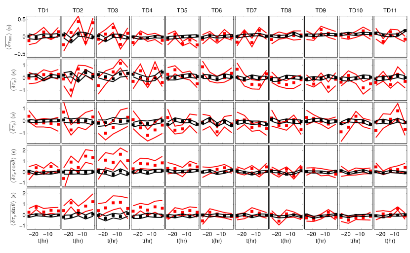
Figure 9.— Spatial and ensemble averages ${\langle\overline{\delta\tau_{\rm mn}}\rangle}$, ${\langle\overline{\delta\tau_{x}}\rangle}$, ${\langle\overline{\delta\tau_{y}}\rangle}$, ${\langle\overline{\delta\tau_{x}\cos{\theta}}\rangle}$, and ${\langle\overline{\delta\tau_{y}\sin{\theta}}\rangle}$ for the subsample of eleven PE regions (red) and all of the NE regions (black). Notice that the plotting ranges for all variables except ${\langle\overline{\delta\tau_{\rm mn}}\rangle}$ are different than in Figure 6.

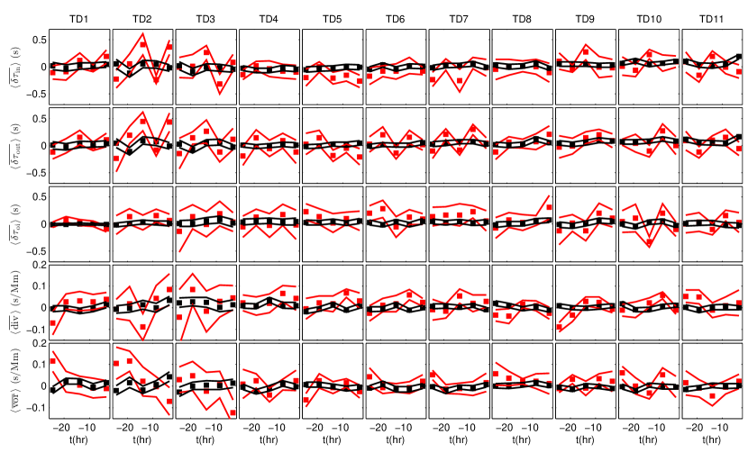
Figure 10.— Spatial and ensemble averages ${\langle\overline{\delta\tau_{\rm in}}\rangle}$, ${\langle\overline{\delta\tau_{\rm out}}\rangle}$, ${\langle\overline{\delta\tau_{\rm oi}}\rangle}$, $\langle\overline{\rm div}\rangle$, and $\langle\overline{\rm vor}\rangle$ for the subsample of eleven PE regions (red) and all of the NE regions (black). Notice that the plotting ranges for all variables except ${\langle\overline{\delta\tau_{\rm in}}\rangle}$ and ${\langle\overline{\delta\tau_{\rm out}}\rangle}$ are different than in Figure 7.

5. Discussion

We have applied helioseismic holography to 107 pre-emergence active regions and an equal number of areas where no active region emergence occurred. The sample of emerging active regions, as described in Paper I, spans a wide range of eventual sizes and temporal evolution profiles of $B_{r}$; in addition, these active regions emerge into a variety of magnetic contexts. We present single-region examples, but concentrate herein primarily on averages over the samples in the two populations, and on spatial (and ensemble) averages over the central emergence area.

We have found differences in the average seismic signatures between these two populations. The pre-emergence regions show a ${\delta\tau}_{\rm mn}$ that is reduced by several tenths of a second (in all but the shallowest layers), compared to the non-emergence population. There are persistent anti-symmetric features with magnitudes of up to 2 s in ${\delta\tau}_{x}$ and ${\delta\tau}_{y}$ in the shallow filters. These features may qualitatively suggest a converging flow of order 15 m s^-1. No clear statistically significant differences between the average pre-emergence sample and no-emergence sample were found in the vorticity and only hints seen in the divergence.

However, two caveats must be included in the above summary. First, there exists a weak but persistent average magnetic signal at the emergence site prior to detectable flux emergence; it strengthens as the emergence start approaches, as does the magnitude of the co-spatial ${\delta\tau}_{\rm mn}$ deficit. The causal relationship between these features is not clear: does the change in wave speed and the apparent flow result from the surface magnetic field? has the magnetic field collected at the emergence site because of the converging flows?

Another possibility is that this is another example of a bias in the selection of the samples used in this investigation, and our results are a consequence of emergence happening preferentially at the boundary between supergranules. Our non-emergence sample has no preferential location compared to supergranules, but if the emergence locations are preferentially centered on the boundary between supergranules, this would result in flows towards the emergence location. The flows would not then be converging on the emergence location, but rather the emergence location would be between neighboring diverging flows from the supergranules.

The depth of the antisymmetric features in ${\langle\delta\tau_{x}\rangle}$ and ${\langle\delta\tau_{y}\rangle}$ approximately corresponds to the typical depths to which supergranular flow is detected, $\approx 5$ Mm, and a typical supergranule lifetime of 1-2 days is at least as long as the time considered here (Rieutord & Rincon, 2010). Further, the presence of surface magnetic field prior to emergence could also be a result of the tendency for magnetic flux to concentrate in the boundaries between supergranules. Finally, this might also account for the comparatively weak signature of emergence in ${\langle\overline{\delta\tau_{\rm oi}}\rangle}$, when compared to the signature in ${\langle\overline{\delta\tau_{x}\cos{\theta}}\rangle}$, and ${\langle\overline{\delta\tau_{y}\sin{\theta}}\rangle}$, as this is not a simple converging flow. Thus we may not be seeing a signal of emergence so much as a signal of supergranules. This in itself would be an interesting result, as it demonstrates a preference for emergence to occur at the boundary between supergranules.

We note, however, the typical flow speed for a supergranule of several hundred meters per second (Rieutord & Rincon, 2010) is an order of magnitude larger than our ensemble average of observed travel time shifts. This could be a result of imperfect alignment between the boundary and the emergence location, keeping in mind that our averaging disk is large compared to a typical supergranule size. By averaging over multiple supergranules for each emergence, the average travel time difference would be greatly reduced. The difference in flow speeds could also result from weakening flow toward the edge of the supergranule.

In Paper III we attempt to disentangle the relationships among some of the parameters where a difference between PE and NE samples is found. For example, do the ${\delta\tau}_{\rm mn}$ maps contain information that is not in the maps of $|B_{r}|$? In addition, Paper III uses Discriminant Analysis (Kendall et al., 1983) to determine which measurements are best able to distinguish the PE and NE populations, as a complement to the ensemble averaging performed here.

Second, when a subset of eleven “best” active region candidates (emerging with a fast, monotonically-increasing flux history into an essentially field-free area) were considered, some of the differences described above disappeared. Specifically, there were no longer detectable differences in ${\langle\overline{\delta\tau_{\rm mn}}\rangle}$ or ${\langle\overline{\delta\tau_{\rm oi}}\rangle}$. However, the direction-weighted ${\langle\overline{\delta\tau_{x}\cos\theta}\rangle}$ and ${\langle\overline{\delta\tau_{y}\sin\theta}\rangle}$ parameters continue to show a statistically significant difference (of up to 2 s), for moderate depths. This subset includes the much-studied NOAA AR 10488 (see Paper I for the full list).

The results presented here place strong constraints on models of the emergence of AR. We have shown that in the $\approx 24$ hours before emergence that the sub-surface flows, averaged over 6 hours, are no more than $\approx 15~{}{\rm m\,s}^{-1}$. This raises the question of the time evolution of the strong (100 m s^-1) retrograde flows suggested by models (e.g. Fan, 2008): why have we not observed these flows? how do these retrograde flows interact with the near-surface shear layer?

It is not clear how to reconcile the results presented here with the strong pre-emergence reduction (of order 10 s) in the mean travel-time seen by Ilonidis et al. (2011). Ilonidis et al. (2011) suggest that this signature may be caused by a rising flux concentration crossing upwards through the depth of 60 Mm, where their analysis is sensitive. Here, we use measurements that are sensitive to depths shallower than about 20 Mm, and see no signature in ${\delta\tau}_{\rm mn}$ larger than a fraction of a second. Further measurements are needed to connect these two conclusions; why does the helioseismic impact of the rising tube all but disappear as the tube approaches the photosphere?

We have found that, on average for our pre-emergence sample, there are surface magnetic fields present at the emergence site but which vary only slowly (see Fig. 10 of Paper I, ) over the day before flux emergence begins in earnest. As discussed above, this may be due to a preference for emergence to occur at the boundaries between supergranules where “quiet” magnetic flux typically accumulates continuously. As another possibility, we speculate that this may perhaps be a result of the interaction between convection and the rising magnetic fields, i.e., that the portion of the flux that is caught in the fastest upflows arrives at the surface well before the bulk of the flux tube. Yet another possibility may be that flux emergence occurs preferentially into remnant field. A more detailed analysis is needed to disentangle these effects.

The data analysis we have presented here suggests that the rapid emergence process simulated by Cheung et al. (2010) is not typical. Horizontal flows of order km s^-1 extending over tens of Mm would produce signals in ${\delta\tau}_{x}$ and ${\delta\tau}_{y}$ of order tens of seconds – well above our noise level. Notice, however, if flows of this strength were to develop only after the emergence time, they would not appear in the current analysis. The same is true for the retrograde flows seen in the rising flux tube simulations discussed in Fan (2008). The picture we find here is apparently more compatible with the scenario of Stein et al. (2011), in which weak field is brought to the surface by convection, which is itself only weakly altered by the magnetic field.

References

- Barnes et al. (2012) Barnes, G., Leka, K. D., Birch, A. C., & Braun, D. C. 2012, ApJ
- Brandenburg (2005) Brandenburg, A. 2005, ApJ, 625, 539
- Braun (1995) Braun, D. C. 1995, in Astronomical Society of the Pacific Conference Series, Vol. 76, GONG 1994. Helio- and Astro-Seismology from the Earth and Space, ed. R. K. Ulrich, E. J. Rhodes Jr., & W. Dappen, 250
- Braun (2012) Braun, D. C. 2012, Science, 336, 296
- Braun et al. (1987) Braun, D. C., Duvall, J. T. L., & Labonte, B. J. 1987, ApJ, 319, L27
- Braun et al. (1992) Braun, D. C., Duvall, J. T. L., Labonte, B. J., Jefferies, S. M., Harvey, J. W., & Pomerantz, M. A. 1992, ApJ, 391, L113
- Chang et al. (1997) Chang, H., Chou, D., Labonte, B., & The TON Team. 1997, Nature, 389, 825
- Chang et al. (1999) Chang, H., Chou, D., & Sun, M. 1999, ApJ, 526, L53
- Cheung et al. (2010) Cheung, M. C. M., Rempel, M., Title, A. M., & Schüssler, M. 2010, ApJ, 720, 233
- Chou et al. (1995) Chou, D., Sun, M., Huang, T., Lai, S., Chi, P., Ou, K., Wang, C., Lu, J., Chu, A., Niu, C., Mu, T., Chen, K., Chou, Y., Jimenez, A., Rabello-Soares, M. C., Chao, H., Ai, G., Wang, G., Zirin, H., Marquette, W., & Nenow, J. 1995, Sol. Phys., 160, 237
- Couvidat et al. (2005) Couvidat, S., Gizon, L., Birch, A. C., Larsen, R. M., & Kosovichev, A. G. 2005, ApJS, 158, 217
- Duvall et al. (1993) Duvall, J. T. L., Jefferies, S. M., Harvey, J. W., & Pomerantz, M. A. 1993, Nature, 362, 430
- Duvall et al. (1997) Duvall, J. T. L., Kosovichev, A. G., Scherrer, P. H., Bogart, R. S., Bush, R. I., de Forest, C., Hoeksema, J. T., Schou, J., Saba, J. L. R., Tarbell, T. D., Title, A. M., Wolfson, C. J., & Milford, P. N. 1997, Sol. Phys., 170, 63
- Fan (2008) Fan, Y. 2008, ApJ, 676, 680
- Fan (2009) —. 2009, Living Reviews in Solar Physics, 6, 4
- Gizon & Birch (2005) Gizon, L. & Birch, A. C. 2005, Living Reviews in Solar Physics, 2, 6
- Gizon et al. (2010) Gizon, L., Birch, A. C., & Spruit, H. C. 2010, ARA&A, 48, 289
- Hartlep et al. (2011) Hartlep, T., Kosovichev, A. G., Zhao, J., & Mansour, N. N. 2011, Sol. Phys., 268, 321
- Hill (1988) Hill, F. 1988, ApJ, 333, 996
- Ilonidis et al. (2011) Ilonidis, S., Zhao, J., & Kosovichev, A. 2011, Science, 333, 993
- Jensen et al. (2001) Jensen, J. M., Duvall, J. T. L., Jacobsen, B. H., & Christensen-Dalsgaard, J. 2001, ApJ, 553, L193
- Kendall et al. (1983) Kendall, M., Stuart, A., & Ord, J. K. 1983, The Advanced Theory of Statistics, 4th edn., Vol. 3 (New York: Macmillan Publishing Co., Inc)
- Komm et al. (2009) Komm, R., Howe, R., & Hill, F. 2009, Sol. Phys., 258, 13
- Komm et al. (2011) —. 2011, Sol. Phys., 268, 407
- Komm et al. (2008) Komm, R., Morita, S., Howe, R., & Hill, F. 2008, ApJ, 672, 1254
- Kosovichev (2009) Kosovichev, A. G. 2009, Space Sci. Rev., 144, 175
- Kosovichev & Duvall (2008) Kosovichev, A. G. & Duvall, Jr., T. L. 2008, in Astronomical Society of the Pacific Conference Series, Vol. 383, Subsurface and Atmospheric Influences on Solar Activity, ed. R. Howe, R. W. Komm, K. S. Balasubramaniam, & G. J. D. Petrie, 59
- Leka et al. (2012) Leka, K. D., Barnes, G., Birch, A. C., Gonzalez-Hernandez, I., Dunn, T., Javornik, B., & Braun, D. C. 2012, ApJ
- Lindsey & Braun (2000) Lindsey, C. & Braun, D. C. 2000, Sol. Phys., 192, 261
- Lindsey & Braun (2005) —. 2005, ApJ, 620, 1107
- Pearson (1990) Pearson, F. 1990, Map projections : theory and applications (Boca Raton, Fla.: CRC Press)
- Rieutord & Rincon (2010) Rieutord, M. & Rincon, F. 2010, Living Reviews in Solar Physics, 7, 2
- Stein et al. (2011) Stein, R. F., Lagerfjärd, A., Nordlund, Å., & Georgobiani, D. 2011, Sol. Phys., 268, 271
- Zhao et al. (2004) Zhao, J., Kosovichev, A. G., & Duvall, J. T. L. 2004, ApJ, 607, L135
- Zharkov & Thompson (2008) Zharkov, S. & Thompson, M. J. 2008, Sol. Phys., 251, 369