Convex and Scalable Weakly Labeled SVMs

Abstract

In this paper, we study the problem of learning from weakly labeled data, where labels of the training examples are incomplete. This includes, for example, (i) semi-supervised learning where labels are partially known; (ii) multi-instance learning where labels are implicitly known; and (iii) clustering where labels are completely unknown. Unlike supervised learning, learning with weak labels involves a difficult Mixed-Integer Programming (MIP) problem. Therefore, it can suffer from poor scalability and may also get stuck in local minimum. In this paper, we focus on SVMs and propose the WellSVM via a novel label generation strategy. This leads to a convex relaxation of the original MIP, which is at least as tight as existing convex Semi-Definite Programming (SDP) relaxations. Moreover, the WellSVM can be solved via a sequence of SVM subproblems that are much more scalable than previous convex SDP relaxations. Experiments on three weakly labeled learning tasks, namely, (i) semi-supervised learning; (ii) multi-instance learning for locating regions of interest in content-based information retrieval; and (iii) clustering, clearly demonstrate improved performance, and WellSVM is also readily applicable on large data sets.

Keywords: weakly labeled data, semi-supervised learning, multi-instance learning, clustering, cutting plane, convex relaxation

1 Introduction

Obtaining labeled data is expensive and difficult. For example, in scientific applications, obtaining the labels involves repeated experiments that may be hazardous; in drug prediction, deriving active molecules of a new drug involves expensive expertise that may not even be available. On the other hand, weakly labeled data, where the labels are incomplete, are often ubiquitous in many applications. Therefore, exploiting weakly labeled training data may help improve performance and discover the underlying structure of the data. Indeed, this has been regarded as one of the most challenging tasks in machine learning research (Mitchell, 2006).

Many weak-label learning problems have been proposed. In the following, we summarize several major learning paradigms with weakly labeled data:

• Labels are partially known. A representative example is semi-supervised learning (SSL) (Chapelle et al., 2006b; Zhu, 2006; Zhou and Li, 2010), where most of the training examples are unlabeled and only a few are labeled. SSL improves generalization performance by using the unlabeled examples that are often abundant. In the past decade, SSL has attracted much attention and achieved successful results in diverse applications such as text categorization, image retrieval, and medical diagnosis.

• Labels are implicitly known. Multi-instance learning (MIL) (Dietterich et al., 1997) is the most prominent example in this category. In MIL, training examples are called bags, each of which contains multiple instances. Many real-world objects can be naturally described by multiple instances. For example, an image (bag) usually contains multiple semantic regions, and each region is an instance. Instead of describing an object as a single instance, the multi-instance representation can help separate different semantics within the object. MIL has been successfully applied to diverse domains such as image classification, text categorization, and web mining. The relationship between multi-instance learning and semi-supervised learning has also been discussed in Zhou and Xu (2007).

  In traditional MIL, a bag is labeled positive when it contains at least one positive instance, and is labeled negative otherwise. Although the bag labels are often available, the instance labels are only implicitly known. It is worth noting that identification of the key (or positive) instances from the positive bags can be very useful in many real-world applications. For example, in content-based information retrieval (CBIR), the explicit identification of regions of interest (ROI) can help the user to recognize images that he/she wants quickly (especially when the system returns a large number of images). Similarly, to detect suspect areas in some medical and military applications, a quick scanning of a huge number of images is required. Again, it is very desirable if ROIs can be identified. Besides providing an accurate and efficient prediction, the identification of key instances is also useful in understanding ambiguous objects (Li et al., 2012).

• Labels are totally unknown. This becomes unsupervised learning (Jain and Dubes, 1988), which aims at discovering the underlying structure (or concepts/labels) of the data and grouping similar examples together. Clustering is valuable in data analysis, and is widely used in various domains including information retrieval, computer version, and bioinformatics.

• There are other kinds of weak-label learning problems. For instances, Angluin and Laird (1988) and references therein studied noisy-tolerant problems where the label information is noisy; Sheng et al. (2008) and references therein considered learning from multiple annotation results by different experts in which all the experts are imperfect; Sun et al. (2010) and Bucak et al. (2011) considered weakly labeled data in the context of multi-label learning, whereas Yang et al. (2013) considered weakly labeled data in the context of multi-instance multi-label learning (Zhou et al., 2012).

Unlike supervised learning where the training labels are complete, weak-label learning needs to infer the integer-valued labels of the training examples, resulting in a difficult mixed-integer programming (MIP). To solve this problem, many algorithms have been proposed, including global optimization (Chapelle et al., 2008; Sindhwani et al., 2006) and convex SDP relaxations (Xu et al., 2005; Xu and Schuurmans, 2005; De Bie and Cristianini, 2006; Guo, 2009). Empirical studies have demonstrated their promising performance on small data sets. Although SDP convex relaxations can reduce the training time complexity of global optimization methods from exponential to polynomial, they still cannot handle medium-sized data sets having thousands of examples. Recently, several algorithms resort to using non-convex optimization techniques (such as alternating optimization methods (Andrews et al., 2003; Zhang et al., 2007; Li et al., 2009b) and constrained convex-concave procedure (Collobert et al., 2006; Cheung and Kwok, 2006; Zhao et al., 2008). Although these approaches are often efficient, they can only obtain locally optimal solutions and can easily get stuck in local minima. Therefore, it is desirable to develop a scalable yet convex optimization method for learning with large-scale weakly labeled data. Moreover, unlike several scalable graph-based methods proposed for the transductive setup (Subramanya and Bilmes, 2009; Zhang et al., 2009a; Vapnik, 1998), here we are more interested in inductive learning methods.

In this paper, we will focus on the binary support vector machines (SVM). Extending our preliminary works in Li et al. (2009a, c), we propose a convex weakly labeled SVM (denoted WellSVM (WEakly LabeLed SVM)) via a novel “label generation” strategy. Instead of obtaining a label relation matrix via SDP, WellSVM maximizes the margin by generating the most violated label vectors iteratively, and then combines them via efficient multiple kernel learning techniques. The whole procedure can be formulated as a convex relaxation of the original MIP problem. Furthermore, it can be shown that the learned linear combination of label vector outer-products is in the convex hull of the label space. Since the convex hull is the smallest convex set containing the target non-convex set (Boyd and Vandenberghe, 2004), our formulation is at least as tight as the convex SDP relaxations proposed in Xu et al. (2005), De Bie and Cristianini (2006) and Xu and Schuurmans (2005). Moreover, WellSVM involves a series of SVM subproblems, which can be readily solved in a scalable and efficient manner via state-of-the-art SVM software such as LIBSVM (Fan et al., 2005), SVM-perf (Joachims, 2006), LIBLINEAR (Hsieh et al., 2008) and CVM (Tsang et al., 2006). Therefore, WellSVM scales much better than existing SDP approaches or even some non-convex approaches. Experiments on three common weak-label learning tasks (semi-supervised learning, multi-instance learning, and clustering) validate the effectiveness and scalability of the proposed WellSVM.

The rest of this paper is organized as follows. Section 2 briefly introduces large margin weak-label learning. Section 3 presents the proposed WellSVM and analyzes its time complexity. Section 4 presents detailed formulations on three weak-label learning problems. Section 5 shows some comprehensive experimental results and the last section concludes.

In the following, ${\bf M}\succ 0$ (resp. ${\bf M}\succeq 0$) denotes that the matrix ${\bf M}$ is symmetric and positive definite (pd) (resp. positive semidefinite (psd)). The transpose of vector / matrix (in both the input and feature spaces) is denoted by the superscript ^′, and ${\bf 0},{\bf 1}\in\mathbb{R}^{n}$ denote the zero vector and the vector of all ones, respectively. The inequality ${\bf v}=[v_{1},\ldots,v_{k}]^{\prime}\geq{\bf 0}$ means that $v_{i}\geq 0$ for $i=1,\ldots,k$. Similarly, ${\bf M}\geq{\bf 0}$ means that all elements in the matrix ${\bf M}$ are nonnegative.

2 Large-Margin Weak-Label Learning

We commence with the simpler supervised learning scenario. Given a set of labeled examples $\mathcal{D}=\{{\bf x}_{i},y_{i}\}_{i=1}^{N}$ where ${\bf x}_{i}\in{\cal X}$ is the input and ${y}_{i}\in\{\pm 1\}$ is the output, we aim to find a decision function $f:{\cal X}\rightarrow\{\pm 1\}$ such that the following structural risk functional is minimized:

$$\min_{f}\;\Omega(f)+C\;\ell_{f}(\mathcal{D}).$$ (1)

Here, $\Omega$ is a regularizer related to large margin on $f$, $\ell_{f}(\mathcal{D})$ is the empirical loss on ${\mathcal{D}}$, and $C$ is a regularization parameter that trades off the empirical risk and model complexity. Both $\Omega$ and $\ell_{f}{(\cdot)}$ are problem-dependent. In particular, when $\ell_{f}{(\cdot)}$ is the hinge loss (or its variants), the obtained $f$ is a large margin classifier. It is notable that both $\Omega$ and $L_{f}(\cdot)$ are usually convex. Thus, Equation (1) is a convex problem whose globally optimal solution can be efficiently obtained via various convex optimization techniques.

In weak-label learning, labels are not available on all $N$ training examples, and so also need to be learned. Let $\hat{{\bf y}}=[\hat{y}_{1},\cdots,\hat{y}_{N}]^{\prime}\in\{\pm 1\}^{N}$ be the vector of (known and unknown) labels on all the training examples. The basic idea of large-margin weak-label learning is that the structural risk functional in Equation (1) is minimized w.r.t. both the labeling $\hat{{\bf y}}$ and decision function $f$. Hence, Equation (1) is extended to

$$\min_{\hat{{\bf y}}\in{\cal B}}\;\min_{f}\;\;\;\;\Omega(f)+C\;\ell_{f}(\{{\bf x}_{i},\hat{y}_{i}\}_{i=1}^{N}),$$ (2)

where ${\cal B}$ is a set of candidate label assignments obtained from some domain knowledge. For example, when the positive and negative examples are known to be approximately balanced, we can set ${\cal B}=\{\hat{{\bf y}}\;:\;-\beta\leq\sum_{i=1}^{N}\hat{y}_{i}\leq\beta\}$ where $\beta$ is a small constant controlling the class imbalance.

2.1 State-of-The-Art Approaches

As Equation (2) involves optimizing the integer variables $\hat{{\bf y}}$, it is no longer a convex optimization problem but a mixed-integer program. This can easily suffer from the local minimum problem. Recently, a lot of efforts have been devoted to solve this problem. They can be grouped into three categories. The first strategy optimizes Equation (2) via variants of non-convex optimization. Examples include alternating optimization (Zhang et al., 2009b; Li et al., 2009b; Andrews et al., 2003), in which we alternatively optimize variable $\hat{{\bf y}}$ (or $f$) by keeping the other variable $f$ (or $\hat{{\bf y}}$) constant; constrained convex-concave procedure (CCCP) (also known as DC programming) (Horst and Thoai, 1999; Zhao et al., 2008; Collobert et al., 2006; Cheung and Kwok, 2006), in which the non-convex objective function or constraint is decomposed as a difference of two convex functions; local combinatorial search (Joachims, 1999), in which the labels of two examples in opposite classes are sequentially switched. These approaches are often computationally efficient. However, since they are based on non-convex optimization, they may inevitably get stuck in local minima.

The second strategy obtains the globally optimal solution of Equation (2) via global optimization. Examples include branch-and-bound (Chapelle et al., 2008) and deterministic annealing (Sindhwani et al., 2006). Since they aim at obtaining the globally optimal (instead of the locally optimal) solution, excellent performance can be expected (Chapelle et al., 2008). However, their worst-case computational costs can scale exponentially as the data set size. Hence, these approaches can only be applied to small data sets with just hundreds of training examples.

The third strategy is based on convex relaxations. The original non-convex problem is first relaxed to a convex problem, whose globally optimal solution can be efficiently obtained. This is then rounded to recover an approximate solution of the original problem. If the relaxation is tight, the approximate solution obtained is close to the global optimum of the original problem and good performance can be expected. Moreover, the involved convex programming solver has a time complexity substantially lower than that for global optimization. A prominent example of convex relaxation is the use of semidefinite programming (SDP) techniques (Xu et al., 2005; Xu and Schuurmans, 2005; De Bie and Cristianini, 2006; Guo, 2009), in which a positive semidefinite matrix is used to approximate the matrix of label outer-products. The time complexity of this SDP-based strategy is $O(N^{6.5})$ (Lobo et al., 1998; Nesterov and Nemirovskii, 1987), where $N$ is the data set size, and can be further reduced to $O(N^{4.5})$ (Zhang et al., 2009b; Valizadegan and Jin, 2007). However, this is still expensive for medium-sized data sets with several thousands of examples.

To summarize, existing weak-label learning approaches are not scalable or can be sensitive to initialization. In this paper, we propose the WellSVM algorithm to address these two issues.

3 WellSVM

In this section, we first introduce the SVM dual which will be used as a basic reformulation of our proposal, and then we present the general formulation of WellSVM. Detailed formulations on three common weak-label learning tasks will be presented in Section 4.

3.1 Duals in Large Margin Classifiers

In large margin classifiers, the inner minimization problem of Equation (2) is often cast in the dual form. For example, for the standard SVM without offset, we have $\Omega=\frac{1}{2}\|{\bf w}\|^{2}$ and $\ell_{f}(D)$ is the summed hinge loss. The inner minimization problem is then

$$\min\limits_{{\bf w},\boldsymbol{\xi}} \frac{1}{2}||{\bf w}||_{2}^{2}+C\sum_{i=1}^{N}\xi_{i}$$

s.t. $$\hat{y}_{i}{\bf w}^{\prime}\phi({\bf x}_{i})\geq 1-\xi_{i},\;\;\xi_{i}\geq 0,\;\;i=1\dots,N,$$

where $\phi({\bf x}_{i})$ is the feature map induced by kernel $\kappa$, and its dual is

$$\max\limits_{\boldsymbol{\alpha}} \boldsymbol{\alpha}^{\prime}{\bf 1}-\frac{1}{2}\boldsymbol{\alpha}^{\prime}\big{(}{\bf K}\odot\hat{{\bf y}}\hat{{\bf y}}^{\prime}\big{)}\boldsymbol{\alpha}$$

s.t. $$C{\bf 1}\geq\boldsymbol{\alpha}\geq{\bf 0},$$

where $\boldsymbol{\alpha}\in\mathbb{R}^{N}$ is the dual variable, ${\bf K}\in\mathbb{R}^{N\times N}$ is the kernel matrix defined on the $N$ samples, and $\odot$ is the element-wise product. For more details on the duals of large margin classifiers, interested readers are referred to Schölkopf and Smola (2002) and Cristianini et al. (2002).

In this paper, we make the following assumption on this dual.

Assumption 1

The dual of the inner minimization of Equation (2) can be written as: $\max_{\boldsymbol{\alpha}\in{\cal A}}G(\boldsymbol{\alpha},\hat{{\bf y}})$, where $\boldsymbol{\alpha}=[\alpha_{1},\ldots,\alpha_{N}]^{\prime}$ contains the dual variables and

• ${\cal A}$ is a convex set;

• $G(\boldsymbol{\alpha},\hat{{\bf y}})$ is a concave function in $\boldsymbol{\alpha}$ for any fixed $\hat{{\bf y}}$;

• $g_{{\bf y}}(\boldsymbol{\alpha})=-G(\boldsymbol{\alpha},{\bf y})$ is $\lambda$-strongly convex and $M$-Lipschitz. In other words, $\nabla^{2}g_{{\bf y}}(\boldsymbol{\alpha})-\lambda{\bf I}\succeq 0$, where ${\bf I}$ is the identity matrix, and $\|g_{{\bf y}}(\boldsymbol{\alpha})-g_{{\bf y}}(\bar{\boldsymbol{\alpha}})\|\leq M\|\boldsymbol{\alpha}-\bar{\boldsymbol{\alpha}}\|,\ \forall{\bf y}\in{\cal B},\ \boldsymbol{\alpha},\bar{\boldsymbol{\alpha}}\in{\cal A}$;

• $\forall\hat{{\bf y}}\in{\cal B}$, $lb\leq\max_{\boldsymbol{\alpha}\in{\cal A}}G(\boldsymbol{\alpha},\hat{{\bf y}})\leq ub$, where $lb$ and $ub$ are polynomial in $N$;

• $G(\boldsymbol{\alpha},\hat{{\bf y}})$ can be rewritten as $\bar{G}(\boldsymbol{\alpha},{\bf M})$, where ${\bf M}$ is a psd matrix, and $\bar{G}$ is concave in $\boldsymbol{\alpha}$ and linear in ${\bf M}$.

With this assumption, Equation (2) can be written as

$$\min_{\hat{{\bf y}}\in{\cal B}}\max_{\boldsymbol{\alpha}\in{\cal A}}\;\;\;G(\boldsymbol{\alpha},\hat{{\bf y}}),$$ (3)

Assume that the kernel matrix ${\bf K}$ is pd (i.e., the smallest eigenvalue $\lambda_{\min}>0$) and all its entries are bounded ($|K_{ij}|\leq\upsilon$ for some $\upsilon$). It is easy to see that the following SVM variants satisfy Assumption 1.

• Standard SVM without offset: We have

  $${\cal A} = \{\boldsymbol{\alpha}\;|\;C{\bf 1}\geq\boldsymbol{\alpha}\geq{\bf 0}\},$$

  $$G(\boldsymbol{\alpha},\hat{{\bf y}}) = \boldsymbol{\alpha}^{\prime}{\bf 1}-\frac{1}{2}\boldsymbol{\alpha}^{\prime}\big{(}{\bf K}\odot\hat{{\bf y}}\hat{{\bf y}}^{\prime}\big{)}\boldsymbol{\alpha},$$

  $$\nabla^{2}g_{{\bf y}}(\boldsymbol{\alpha}) = {\bf K}\odot{{\bf y}}{{\bf y}}^{\prime}\succeq\lambda_{\min}({\bf I}\odot{{\bf y}}{{\bf y}}^{\prime})=\lambda_{\min}{\bf I},$$

  $$\|g_{{\bf y}}(\boldsymbol{\alpha})-g_{{\bf y}}(\bar{\boldsymbol{\alpha}})\| \leq (1+C\upsilon N)\sqrt{N}\|\boldsymbol{\alpha}-\bar{\boldsymbol{\alpha}}\|,$$

  $$0 \leq \max_{\boldsymbol{\alpha}\in{\cal A}}G(\boldsymbol{\alpha},\hat{{\bf y}})\leq CN,$$

  $$\bar{G}(\boldsymbol{\alpha},{\bf M}_{\hat{{\bf y}}}) = \boldsymbol{\alpha}^{\prime}{\bf 1}-\frac{1}{2}\boldsymbol{\alpha}^{\prime}\big{(}{\bf K}\odot{\bf M}_{\hat{{\bf y}}}\big{)}\boldsymbol{\alpha},\;\;\;\text{ where }{\bf M}_{\hat{{\bf y}}}=\hat{{\bf y}}\hat{{\bf y}}^{\prime}.$$

• $\nu$-SVM (Schölkopf and Smola, 2002): We have

  $${\cal A} = \{\boldsymbol{\alpha}\;|\;\boldsymbol{\alpha}\geq{\bf 0},\boldsymbol{\alpha}^{\prime}{\bf 1}=1\},$$

  $$G(\boldsymbol{\alpha},\hat{{\bf y}}) = -\frac{1}{2}\boldsymbol{\alpha}^{\prime}\left(({\bf K}+\frac{1}{C}{\bf I})\odot\hat{{\bf y}}\hat{{\bf y}}^{\prime}\right)\boldsymbol{\alpha},$$

  $$\nabla^{2}g_{{\bf y}}(\boldsymbol{\alpha}) = \left({\bf K}+\frac{1}{C}{\bf I}\right)\odot{{\bf y}}{{\bf y}}^{\prime}\succeq\left(\lambda_{\min}+\frac{1}{C}\right)\;\big{(}{\bf I}\odot{{\bf y}}{{\bf y}}^{\prime}\big{)}=\left(\lambda_{\min}+\frac{1}{C}\right){\bf I},$$

  $$\|g_{{\bf y}}(\boldsymbol{\alpha})-g_{{\bf y}}(\bar{\boldsymbol{\alpha}})\| \leq \left(\upsilon+\frac{1}{C}\right)N\sqrt{N}\|\boldsymbol{\alpha}-\bar{\boldsymbol{\alpha}}\|,$$

  $$-\frac{1}{2}\left(\upsilon+\frac{1}{C}\right) \leq \max_{\boldsymbol{\alpha}\in{\cal A}}G(\boldsymbol{\alpha},\hat{{\bf y}})\leq 0,$$

  $$\bar{G}(\boldsymbol{\alpha},{\bf M}_{\hat{{\bf y}}}) = -\frac{1}{2}\boldsymbol{\alpha}^{\prime}\left(({\bf K}+\frac{1}{C}{\bf I})\odot{\bf M}_{\hat{{\bf y}}}\right)\boldsymbol{\alpha}.$$

3.2 WellSVM

Interchanging the order of $\max_{\boldsymbol{\alpha}\in{\cal A}}$ and $\min_{\hat{{\bf y}}\in{\cal B}}$ in Equation (3), we obtain the proposed WellSVM:

$$(\mbox{{WellSVM}})\;\;\;\;\max_{\boldsymbol{\alpha}\in{\cal A}}\min_{\hat{{\bf y}}\in{\cal B}}\;\;\;G(\boldsymbol{\alpha},\hat{{\bf y}}).$$ (4)

Using the minimax theorem (Kim and Boyd, 2008), the optimal objective of Equation (3) upper-bounds that of Equation (4). Moreover, Equation (4) can be transformed as

$$\!\!\!\max\limits_{\boldsymbol{\alpha}\in{\cal A}}\!\!\! \Big{\{}\max_{\theta}\!\! \!\theta$$

s.t. $$\!\!G(\boldsymbol{\alpha},\hat{{\bf y}}_{t})\geq\theta,\;\forall\hat{{\bf y}}_{t}\in{\cal B}\Big{\}},$$

from which we obtain the following Proposition.

Proposition 1

The objective of WellSVM can be rewritten as the following optimization problem:

$$\min_{\boldsymbol{\mu}\in{\cal M}}\max_{\boldsymbol{\alpha}\in{\cal A}}\sum_{t:\hat{{\bf y}}_{t}\in{\cal B}}\mu_{t}G(\boldsymbol{\alpha},\hat{{\bf y}}_{t}),$$ (6)

where $\boldsymbol{\mu}$ is the vector of $\mu_{t}$’s, ${\cal M}$ is the simplex $\{\boldsymbol{\mu}\;|\;\sum_{t}\mu_{t}=1,\mu_{t}\geq 0\}$, and $\hat{{\bf y}}_{t}\in{\cal B}$.

Proof  For the inner optimization in Equation (3.2), let $\mu_{t}\geq 0$ be the dual variable for each constraint. Its Lagrangian can be obtained as

$$\theta+\sum_{t:\hat{{\bf y}}_{t}\in{\cal B}}\mu_{t}\Big{(}G(\boldsymbol{\alpha},\hat{{\bf y}}_{t})-\theta\Big{)}.$$

Setting the derivative w.r.t. $\theta$ to zero, we have $\sum_{t}\mu_{t}=1$. We can then replace the inner optimization subproblem with its dual and Equation (3.2) becomes:

$$\max_{\boldsymbol{\alpha}\in{\cal A}}\min_{\boldsymbol{\mu}\in{\cal M}}\sum_{t:\hat{{\bf y}}_{t}\in{\cal B}}\mu_{t}G(\boldsymbol{\alpha},\hat{{\bf y}}_{t})=\min_{\boldsymbol{\mu}\in{\cal M}}\max_{\boldsymbol{\alpha}\in{\cal A}}\sum_{t:\hat{{\bf y}}_{t}\in{\cal B}}\mu_{t}G(\boldsymbol{\alpha},\hat{{\bf y}}_{t}).$$

Here, we use the fact that the objective function is convex in $\boldsymbol{\mu}$ and concave in $\boldsymbol{\alpha}$.  

Recall that $G(\boldsymbol{\alpha},\hat{{\bf y}})$ is concave in $\boldsymbol{\alpha}$. Thus, the constraints in Equation (3.2) are convex. It is evident that the objective in Equation (3.2) is linear in both $\boldsymbol{\alpha}$ and $\theta$. Therefore, Equation (3.2) is a convex problem. In other words, WellSVM is a convex relaxation of Equation (2).

3.3 Tighter than SDP Relaxations

In this section, we compare our minimax relaxation with SDP relaxations. It is notable that the SVM without offset is always employed by previous SDP relaxations (Xu et al., 2005; Xu and Schuurmans, 2005; De Bie and Cristianini, 2006).

Recall the symbols in Section 3.1. Define

$${\cal Y}_{0}=\big{\{}{\bf M}\;|\;{\bf M}={\bf M}_{\hat{{\bf y}}},\;\;\hat{{\bf y}}\in{\cal B}\big{\}}.$$

The original mixed-integer program in Equation (3) is the same as

$$\min_{{\bf M}\in{\cal Y}_{0}}\max_{\boldsymbol{\alpha}\in{\cal A}}\;\bar{G}(\boldsymbol{\alpha},{\bf M}).$$ (7)

Define ${\cal Y}_{1}=\big{\{}{\bf M}\;|\;{\bf M}=\sum_{t:\hat{{\bf y}}_{t}\in{\cal B}}\mu_{t}{\bf M}_{\hat{{\bf y}}_{t}},\;\;\boldsymbol{\mu}\in{\cal M}\big{\}}$. Our minimax relaxation in Equation (6) can be written as

$$\min_{\boldsymbol{\mu}\in{\cal M}}\max_{\boldsymbol{\alpha}\in{\cal A}}\sum_{t:\hat{{\bf y}}_{t}\in{\cal B}}\mu_{t}\bar{G}(\boldsymbol{\alpha},{\bf M}_{\hat{{\bf y}}_{t}}) = \min_{\boldsymbol{\mu}\in{\cal M}}\max_{\boldsymbol{\alpha}\in{\cal A}}\bar{G}\left(\boldsymbol{\alpha},\sum_{t:\hat{{\bf y}}_{t}\in{\cal B}}\mu_{t}{\bf M}_{\hat{{\bf y}}_{t}}\right)$$ (8)

$$= \min_{{\bf M}\in{\cal Y}_{1}}\max_{\boldsymbol{\alpha}\in{\cal A}}\;\bar{G}(\boldsymbol{\alpha},{\bf M}).$$

On the other hand, the SDP relaxations in Xu et al. (2005); Xu and Schuurmans (2005) and De Bie and Cristianini (2006) are of the form

$$\min_{{\bf M}\in{\cal Y}_{2}}\max_{\boldsymbol{\alpha}\in{\cal A}}\;\bar{G}(\boldsymbol{\alpha},{\bf M}),$$

where ${\cal Y}_{2}=\big{\{}{\bf M}\;|\;{\bf M}\succeq 0,{\bf M}\in{\cal M}_{{\cal B}}\big{\}}$, and ${\cal M}_{{\cal B}}$ is a convex set related to ${\cal B}$. For example, in the context of clustering, Xu et al. (2005) used ${\cal B}=\{\hat{{\bf y}}|-\beta\leq{\bf 1}^{\prime}\hat{{\bf y}}\leq\beta\}$, where $\beta$ is a parameter controlling the class imbalance, and ${\cal M}_{{\cal B}}$ is defined as

$${\cal M}_{{\cal B}}^{\text{clustering}}= \Big{\{}{\bf M}=[m_{ij}]\;| -1\leq m_{ij}\leq 1;m_{ii}=1,m_{ij}=m_{ji},$$

$$m_{ik}\geq m_{ij}+m_{jk}-1,m_{jk}\geq-m_{ij}-m_{ik}-1,$$

$$-\beta\leq\sum_{i=1}^{N}m_{ij}\leq\beta,\;\;\forall i,j,k=1,\dots,N\Big{\}}.$$

It is easy to verify that ${\cal Y}_{0}\subseteq{\cal Y}_{2}$ and ${\cal Y}_{2}$ is convex. Similarly, in semi-supervised learning, Xu and Schuurmans (2005) and De Bie and Cristianini (2006) defined ${\cal M}_{{\cal B}}$ as a subset of ${\cal M}_{{\cal B}}^{\text{clustering}}$. Again, ${\cal Y}_{0}\subseteq{\cal Y}_{2}$ and ${\cal Y}_{2}$ is convex.

Theorem 1

The relaxation of WellSVM is at least as tight as the SDP relaxations in Xu et al. (2005); Xu and Schuurmans (2005) and De Bie and Cristianini (2006).

Proof  Note that ${\cal Y}_{1}$ is the convex hull of ${\cal Y}_{0}$, that is, the smallest convex set containing ${\cal Y}_{0}$ (Boyd and Vandenberghe, 2004). Therefore, Equation (8) gives the tightest convex relaxation of Equation (7), that is, ${\cal Y}_{1}\subseteq{\cal Y}_{2}$. In other words, our relaxation is at least as tight as SDP relaxations.  

3.4 Cutting Plane Algorithm by Label Generation

It appears that existing convex optimization techniques can be readily used to solve the convex problem in Equation (6), or equivalently Equation (3.2). However, note that there can be an exponential number of constraints in Equation (3.2), and so a direct optimization is computationally intractable. Fortunately, typically not all these constraints are active at optimality, and including only a subset of them can lead to a very good approximation of the original optimization problem. Therefore, we can apply the cutting plane method (Kelley, 1960).

The cutting plane algorithm is described in Algorithm 1. First, we initialize a label vector $\hat{{\bf y}}$ and the working set ${\cal C}$ to $\{\hat{{\bf y}}\}$, and obtain $\boldsymbol{\alpha}$ from

$$\min_{\boldsymbol{\mu}\in{\cal M}}\max_{\boldsymbol{\alpha}\in{\cal A}}\sum_{t:\hat{{\bf y}}_{t}\in{\cal C}}\mu_{t}G(\boldsymbol{\alpha},\hat{{\bf y}}_{t})$$ (9)

via standard supervised learning methods. Then, a violated label vector $\hat{{\bf y}}$ in Equation (3.2) is generated and added to ${\cal C}$. The process is repeated until the termination criterion is met. Since the size of the working set ${\cal C}$ is often much smaller than that of ${\cal B}$, one can use existing convex optimization techniques to obtain $\boldsymbol{\alpha}$ from Equation (9).

For the non-convex optimization methods reviewed in Section 2.1, a new label assignment for the unlabeled data is also generated in each iteration. However, they are very different from our proposal. First, those algorithms do not take the previous label assignments into account, while, as will be seen in Section 4.1.2, our WellSVM aims to learn a combination of previous label assignments. Moreover, they update the label assignment to approach a locally optimal solution, while our WellSVM aims to obtain a tight convex relaxation solution.

Algorithm 1 Cutting plane algorithm for WellSVM.

1:  Initialize $\hat{{\bf y}}$ and ${\cal C}=\emptyset$.

2:  repeat

3:     Update ${\cal C}\leftarrow\{\hat{{\bf y}}\}\bigcup{\cal C}$.

4:     Obtain the optimal $\boldsymbol{\alpha}$ from Equation (9).

5:     Generate a violated $\hat{{\bf y}}$.

6:  until $G(\boldsymbol{\alpha},\hat{{\bf y}})>\min_{{\bf y}\in{\cal C}}G(\boldsymbol{\alpha},{{\bf y}})-\epsilon$ (where $\epsilon$ is a small constant) or the decrease of objective value is smaller than a threshold.

3.5 Computational Complexity

The key to analyzing the running time of Algorithm 1 is its convergence rate, and we have the following Theorem.

Theorem 2

Let $p^{(t)}$ be the optimal objective value of Equation (9) at the $t$-th iteration. Then,

$$p^{(t+1)}\leq p^{(t)}-\eta,$$ (10)

where $\eta=\Big{(}\frac{-c+\sqrt{c^{2}+4\epsilon}}{2}\Big{)}^{2}$, and $c=M\sqrt{2/\lambda}$.

Proof is in Appendix A. From Theorem 2, we can obtain the following convergence rate.

Proposition 2

Algorithm 1 converges in no more than $\frac{p^{(1)}-p^{*}}{\eta}$ iterations, where $p^{*}$ is the optimal objective value of WellSVM.

According to Assumption 1, we have $p^{*}=\min_{\hat{{\bf y}}\in{\cal B}}\max_{\boldsymbol{\alpha}\in{\cal A}}G(\boldsymbol{\alpha},\hat{{\bf y}})\geq lb$ and $p^{(1)}=\max_{\boldsymbol{\alpha}\in{\cal A}}G(\boldsymbol{\alpha},\hat{{\bf y}})\leq ub$. Moreover, recall that $lb$ and $ub$ are polynomial in $N$. Thus, Proposition 2 shows that with the use of the cutting plane algorithm, the number of active constraints only scales polynomially in $N$. In particular, as discussed in Section 3.1, for the $\nu$-SVM, $lb=-\frac{1}{2}(\upsilon+\frac{1}{C})$ and $ub=0$, both of which are unrelated to $N$. Thus, the number of active constraints only scales as $O(1)$.

Proposition 2 can be further refined by taking the search effort of a violated label into account. The proof is similar to that of Theorem 2.

Proposition 3

Let $\epsilon_{r}\geq\epsilon$, $\forall r=1,2,\ldots$, be the magnitude of the violation of a violated label in the $r$-th iteration, that is, $\epsilon_{r}=\min_{{\bf y}\in{\cal C}_{r}}G(\boldsymbol{\alpha},{{\bf y}})-G(\boldsymbol{\alpha},\hat{{\bf y}}^{r})$, where ${\cal C}_{r}$ and $\hat{{\bf y}}^{r}$ denote the set of violated labels and the violated label obtained in the $r$-th iteration, respectively. Let $\eta_{r}=\Big{(}\frac{-c+\sqrt{c^{2}+4\epsilon_{r}}}{2}\Big{)}^{2}$. Then, Algorithm 1 converges in no more than $R$ iterations where $\sum_{r=1}^{R}\eta_{r}\geq p^{(1)}-p^{*}$.

Hence, the more effort is spent on finding a violated label, the faster is the convergence. This represents a trade-off between the convergence rate and cost in each iteration.

We will show in Section 4 that step 4 of Algorithm 1 can be addressed via multiple kernel learning techniques which only involve a series of SVM subproblems that can be solved efficiently by state-of-the-art SVM software such as LIBSVM (Fan et al., 2005) and LIBLINEAR (Hsieh et al., 2008), while step 5 can be efficiently addressed by sorting. Therefore, the total time complexity of WellSVM scales as the existing SVM solvers, and is significantly faster than SDP relaxations.

4 Three Weak-Label Learning Problems

In this section, we present the detailed formulations of WellSVM on three common weak-label learning tasks, namely, semi-supervised learning (Section 4.1), multi-instance learning (Section 4.2), and clustering (Section 4.3).

4.1 Semi-Supervised Learning

In semi-supervised learning, not all the training labels are known. Let ${\mathcal{D}}_{{\mathcal{L}}}=\{{\bf x}_{i},y_{i}\}_{i=1}^{l}$ and ${\mathcal{D}}_{{\mathcal{U}}}=\{{\bf x}_{j}\}_{j=l+1}^{N}$ be the sets of labeled and unlabeled examples, respectively, and ${{\mathcal{L}}}=\{1,\ldots,l\}$ (resp. ${\mathcal{U}}=\{l+1,\ldots,N\}$) be the index set of the labeled (resp. unlabeled) examples. In semi-supervised learning, unlabeled data are typically much more abundant than labeled data, that is, $N-l\gg l$. Hence, one can obtain a trivially “optimal” solution with infinite margin by assigning all the unlabeled examples to the same label. To prevent such a useless solution, Joachims (1999) introduced the balance constraint

$$\frac{{\bf 1}^{\prime}\hat{{\bf y}}_{{\mathcal{U}}}}{N-l}=\frac{{\bf 1}^{\prime}{{\bf y}}_{{\mathcal{L}}}}{l},$$

where $\hat{{\bf y}}=[\hat{y}_{1},\cdots,\hat{y}_{N}]^{\prime}$ is the vector of learned labels on both labeled and unlabeled examples, ${\bf y}_{{\mathcal{L}}}=[y_{1},\dots,y_{l}]^{\prime}$, and $\hat{{\bf y}}_{{\mathcal{U}}}=[\hat{y}_{l+1},\dots,\hat{y}_{N}]^{\prime}$. Let $\Omega=\frac{1}{2}\|{\bf w}\|^{2}$ and $\ell_{f}({\mathcal{D}})$ be the sum of hinge loss values on both labeled and unlabeled data, Equation (2) leads to

$$\min_{\hat{{\bf y}}\in{\cal B}}\min\limits_{{\bf w},\boldsymbol{\xi}} \frac{1}{2}||{\bf w}||_{2}^{2}+C_{1}\sum_{i=1}^{l}\xi_{i}+C_{2}\sum_{i=l+1}^{N}\xi_{i}$$

s.t. $$\hat{y}_{i}{\bf w}^{\prime}\phi({\bf x}_{i})\geq 1-\xi_{i},\;\;\xi_{i}\geq 0,\;\;i=1\dots,N,$$

where ${\cal B}=\{\hat{{\bf y}}\;|\;\hat{{\bf y}}=[\hat{{\bf y}}_{{\mathcal{L}}};\hat{{\bf y}}_{{\mathcal{U}}}],\hat{{\bf y}}_{{\mathcal{L}}}={\bf y}_{{\mathcal{L}}},\hat{{\bf y}}_{{\mathcal{U}}}\in\{\pm 1\}^{N-l};\frac{{\bf 1}^{\prime}\hat{{\bf y}}_{{\mathcal{U}}}}{N-l}=\frac{{\bf 1}^{\prime}{{\bf y}}_{{\mathcal{L}}}}{l}\}$, and $C_{1},C_{2}$ trade off model complexity and empirical losses on the labeled and unlabeled data, respectively. The inner minimization problem can be rewritten in its dual, as:

$$\min_{\hat{{\bf y}}\in{\cal B}}\max_{\boldsymbol{\alpha}\in{\cal A}} G(\boldsymbol{\alpha},\hat{{\bf y}}):={\bf 1}^{\prime}\boldsymbol{\alpha}-\frac{1}{2}\boldsymbol{\alpha}^{\prime}\Big{(}{\bf K}\odot\hat{{\bf y}}\hat{{\bf y}}^{\prime}\Big{)}\boldsymbol{\alpha},$$ (11)

where $\boldsymbol{\alpha}=[\alpha_{1},\dots,\alpha_{N}]^{\prime}$ is the vector of dual variables, and ${\cal A}=\{\boldsymbol{\alpha}\;\big{|}\;C_{1}\geq\alpha_{i}\geq 0,C_{2}\geq\alpha_{j}\geq 0,i\in{\mathcal{L}},j\in{\mathcal{U}}\}$.

Using Proposition 1, we have

$$\min_{\boldsymbol{\mu}\in{\cal M}}\max_{\boldsymbol{\alpha}\in{\cal A}}\;\;{\bf 1}^{\prime}\boldsymbol{\alpha}-\frac{1}{2}\boldsymbol{\alpha}^{\prime}\Big{(}\sum_{t:\hat{{\bf y}}_{t}\in{\cal B}}\mu_{t}{\bf K}\odot\hat{{\bf y}}_{t}\hat{{\bf y}}_{t}^{\prime}\Big{)}\boldsymbol{\alpha},$$ (12)

which is a convex relaxation of Equation (11). Note that $G(\boldsymbol{\alpha},\hat{{\bf y}})$ can be rewritten as $\bar{G}(\boldsymbol{\alpha},{\bf M}_{{\bf y}})={\bf 1}^{\prime}\boldsymbol{\alpha}-\frac{1}{2}\boldsymbol{\alpha}^{\prime}\Big{(}{\bf K}\odot{\bf M}_{{\bf y}}\Big{)}\boldsymbol{\alpha}$, where $\bar{G}$ is concave in $\boldsymbol{\alpha}$ and linear in ${\bf M}_{{\bf y}}$. Hence, according to Theorem 1, WellSVM is at least as tight as the SDP relaxations in Xu and Schuurmans (2005) and De Bie and Cristianini (2006).

Notice the similarity with standard SVM, which involves a single kernel matrix ${\bf K}\odot\hat{{\bf y}}\hat{{\bf y}}^{\prime}$. Hence, Equation (12) can be regarded as multiple kernel learning (MKL) (Lanckriet et al., 2004), where the target kernel matrix is a convex combination of $|{\cal B}|$ base kernel matrices $\{{\bf K}\odot\hat{{\bf y}}_{t}\hat{{\bf y}}_{t}^{\prime}\}_{t:\hat{{\bf y}}_{t}\in{\cal B}}$, each of which is constructed from a feasible label vector $\hat{{\bf y}}_{t}\in{\cal B}$.

4.1.1 Algorithm

From Section 3, the cutting plane algorithm is used to solve Equation (12). There are two important issues that have to be addressed in the use of cutting plane algorithms. First, how to efficiently solve the MKL optimization problem? Second, how to efficiently find a violated $\hat{{\bf y}}$? These will be addressed in Sections 4.1.2 and 4.1.3, respectively.

4.1.2 Multiple Label-Kernel Learning

In recent years, a lot of efforts have been devoted on efficient MKL approaches. Lanckriet et al. (2004) first proposed the use of quadratically constrained quadratic programming (QCQP) in MKL. Bach et al. (2004) showed that an approximate solution can be efficiently obtained by using sequential minimization optimization (SMO) (Platt, 1999). Recently, Sonnenburg et al. (2006) proposed a semi-infinite linear programming (SILP) formulation which allows MKL to be iteratively solved with standard SVM solver and linear programming. Rakotomamonjy et al. (2008) proposed a weighted 2-norm regularization with additional constraints on the kernel weights to encourage a sparse kernel combination. Xu et al. (2009) proposed the use of the extended level method to improve its convergence, which is further refined by the MKLGL algorithm (Xu et al., 2010). Extension to nonlinear MKL combinations is also studied recently in Kloft et al. (2009).

Unlike standard MKL problems which try to find the optimal kernel function/matrix for a given set of labels, here, we have to find the optimal label kernel matrix. In this paper, we use an adaptation of the MKLGL algorithm (Xu et al., 2010) to solve this multiple label-kernel learning (MLKL) problem. More specifically, suppose that the current working set is ${\cal C}=\{\hat{{\bf y}}_{1},\dots,\hat{{\bf y}}_{T}\}$. Note that the feature map corresponding to the base kernel matrix ${\bf K}\odot\hat{{\bf y}}_{t}\hat{{\bf y}}_{t}^{\prime}$ is ${\bf x}_{i}\mapsto\hat{y}_{ti}\phi({\bf x}_{i})$. The MKL problem in Equation (12) thus corresponds to the following primal optimization problem:

$$\min\limits_{\boldsymbol{\mu}\in{\cal M},{\bf W}=[{\bf w}_{1},\dots,{\bf w}_{T}],\boldsymbol{\xi}} \frac{1}{2}\sum_{t=1}^{T}\frac{1}{\mu_{t}}||{\bf w}_{t}||^{2}+C_{1}\sum_{i=1}^{l}\xi_{i}+C_{2}\sum_{i=l+1}^{N}\xi_{i}$$

s.t. $$\sum_{t=1}^{T}\hat{y}_{ti}{\bf w}_{t}^{\prime}\phi({\bf x}_{i})\geq 1-\xi_{i},\;\;\xi_{i}\geq 0,\;\;i=1,\dots,N.$$

It is easy to verify that its dual can be written as

$$\min\limits_{\boldsymbol{\mu}\in{\cal M}}\max\limits_{\boldsymbol{\alpha}\in{\cal A}} {\bf 1}^{\prime}\boldsymbol{\alpha}-\frac{1}{2}\boldsymbol{\alpha}^{\prime}\Big{(}\sum_{t=1}^{T}\mu_{t}{\bf K}\odot\hat{{\bf y}}_{t}\hat{{\bf y}}_{t}^{\prime}\Big{)}\boldsymbol{\alpha},$$

which is the same as Equation (12). Following MKLGL, we can solve Equation (12) (or, equivalently, Equation (4.1.2)) by iterating the following two steps until convergence.

1. Fix the mixing coefficients $\boldsymbol{\mu}$ of the base kernel matrices and solve Equation (4.1.2). By setting $\tilde{{\bf w}}=[\frac{{\bf w}_{1}}{\sqrt{\mu_{1}}},\ldots,\frac{{\bf w}_{T}}{\sqrt{\mu_{T}}}]^{\prime}$, $\tilde{{\bf x}}_{i}=[\sqrt{\mu_{1}}\phi({\bf x}_{i}),\sqrt{\mu_{2}}\hat{y}_{1i}\hat{y}_{2i}\phi({\bf x}_{i}),\dots,\sqrt{\mu_{T}}\hat{y}_{1i}\hat{y}_{Ti}\phi({\bf x}_{i})]^{\prime}$ and $\tilde{{\bf y}}=\hat{{\bf y}}_{1}$, Equation (4.1.2) can be rewritten as

   $$\min\limits_{\tilde{{\bf w}},\boldsymbol{\xi}} \frac{1}{2}||\tilde{{\bf w}}||^{2}+C_{1}\sum_{i=1}^{l}\xi_{i}+C_{2}\sum_{i=l+1}^{N}\xi_{i}$$

   s.t. $$\tilde{y}_{i}\tilde{{\bf w}}^{\prime}\tilde{{\bf x}}_{i}\geq 1-\xi_{i},\;\;\xi_{i}\geq 0,\;\;i=1,\dots,N,$$

   which is similar to the primal of the standard SVM and can be efficiently handled by state-of-the-art SVM solvers.

2. Fix ${\bf w}_{t}$’s and update $\boldsymbol{\mu}$ in closed-form, as

   $$\mu_{t}=\frac{\|{\bf w}_{t}\|}{\sum_{t^{\prime}=1}^{T}\|{\bf w}_{t^{\prime}}\|},\;\;t=1,\dots,T.$$

In our experiments, this always converges in fewer than $100$ iterations. With the use of warm-start, even faster convergence can be expected.

4.1.3 Finding a Violated Label Assignment

The following optimization problem corresponds to finding the most violated $\hat{{\bf y}}$

$$\min\limits_{\hat{{\bf y}}\in{\cal B}} \;\;\;G(\boldsymbol{\alpha},\hat{{\bf y}})={\bf 1}^{\prime}\boldsymbol{\alpha}-\frac{1}{2}\boldsymbol{\alpha}^{\prime}\Big{(}{\bf K}\odot\hat{{\bf y}}\hat{{\bf y}}^{\prime}\Big{)}\boldsymbol{\alpha}.$$ (14)

The first term in the objective does not relate to $\hat{{\bf y}}$, so Equation (14) is rewritten as

$$\max\limits_{\hat{{\bf y}}\in{\cal B}} \;\;\frac{1}{2}\boldsymbol{\alpha}^{\prime}\Big{(}{\bf K}\odot\hat{{\bf y}}\hat{{\bf y}}^{\prime}\Big{)}\boldsymbol{\alpha}.$$

However, this is a concave QP and cannot be solved efficiently. Note that while the use of the most violated constraint may lead to faster convergence, the cutting plane algorithm only requires the addition of a violated constraint at each iteration (Kelley, 1960; Tsochantaridis et al., 2006). Hence, we propose in the following a simple and efficient method for finding a violated label assignment.

Consider the following equivalent problem:

$$\max\limits_{\hat{{\bf y}}\in{\cal B}}\hat{{\bf y}}^{\prime}{\bf H}\hat{{\bf y}},$$ (15)

where ${\bf H}={\bf K}\odot(\boldsymbol{\alpha}\boldsymbol{\alpha}^{\prime})$ is a psd matrix. Let $\bar{{\bf y}}\in{\cal C}$ be the following suboptimal solution of Equation (15)

$$\bar{{\bf y}}=\mathop{\arg\max}\nolimits_{\hat{{\bf y}}\in{\cal C}}\hat{{\bf y}}^{\prime}{\bf H}\hat{{\bf y}}.$$

Consider an optimal solution of the following optimization problem

$${{\bf y}}^{*}=\operatorname{argmax}\limits_{\hat{{\bf y}}\in{\cal B}}\hat{{\bf y}}^{\prime}{\bf H}\bar{{\bf y}}.$$ (16)

We have the following proposition.

Proposition 4

${{\bf y}}^{*}$ is a violated label assignment if $\bar{{\bf y}}^{\prime}{\bf H}{{\bf y}}^{*}\neq\bar{{\bf y}}^{\prime}{\bf H}\bar{{\bf y}}$.

Proof  From $\hat{{\bf y}}^{\prime}{\bf H}{{\bf y}}^{*}\neq\bar{{\bf y}}^{\prime}{\bf H}\bar{{\bf y}}$, we have ${{\bf y}}^{*}\neq\bar{{\bf y}}$. Suppose that $({{\bf y}}^{*})^{\prime}{\bf H}{{\bf y}}^{*}\leq\bar{{\bf y}}^{\prime}{\bf H}\bar{{\bf y}}$, then $({{\bf y}}^{*})^{\prime}{\bf H}{{\bf y}}^{*}+\bar{{\bf y}}^{\prime}{\bf H}\bar{{\bf y}}-2({{\bf y}}^{*})^{\prime}{\bf H}\bar{{\bf y}}\leq 2\bar{{\bf y}}^{\prime}{\bf H}\bar{{\bf y}}-2({{\bf y}}^{*})^{\prime}{\bf H}\bar{{\bf y}}<0$ which contradicts with $({{\bf y}}^{*})^{\prime}{\bf H}{{\bf y}}^{*}+\bar{{\bf y}}^{\prime}{\bf H}\bar{{\bf y}}-2({{\bf y}}^{*})^{\prime}{\bf H}\bar{{\bf y}}=({{\bf y}}^{*}-\bar{{\bf y}})^{\prime}{\bf H}({{\bf y}}^{*}-\bar{{\bf y}})\geq 0$. So, $({{\bf y}}^{*})^{\prime}{\bf H}{{\bf y}}^{*}>\bar{{\bf y}}^{\prime}{\bf H}\bar{{\bf y}}$ which indicates ${{\bf y}}^{*}$ is a violated label assignment.  

As for solving Equation (16), it is a integer linear program for $\hat{{\bf y}}$. We can rewrite this as

$$\max\limits_{\hat{{\bf y}}} {\bf r}^{\prime}\hat{{\bf y}}={\bf r}_{{\mathcal{L}}}^{\prime}\hat{{\bf y}}_{{\mathcal{L}}}+{\bf r}_{{\mathcal{U}}}^{\prime}\hat{{\bf y}}_{{\mathcal{U}}}$$

s.t. $$\hat{{\bf y}}_{{\mathcal{L}}}={\bf y}_{{\mathcal{L}}},\hat{{\bf y}}_{{\mathcal{U}}}\in\{\pm 1\}^{N-l},\frac{{\bf 1}^{\prime}\hat{{\bf y}}_{{\mathcal{U}}}}{N-l}=\frac{{\bf 1}^{\prime}{{\bf y}}_{{\mathcal{L}}}}{l},$$

where ${\bf r}={\bf H}\bar{{\bf y}}$. Since $\hat{{\bf y}}_{{\mathcal{L}}}$ is constant, we have the following proposition.

Proposition 5

At optimality, $\hat{y}_{i}\geq\hat{y}_{j}$ if $r_{i}>r_{j}$, $i,j\in{\mathcal{U}}$.

Proof  Assume, to the contrary, that the optimal $\hat{{\bf y}}$ does not have the same sorted order as ${\bf r}$. Then, there are two label vectors $\hat{y}_{i}$ and $\hat{y}_{j}$, with $r_{i}>r_{j}$ but $\hat{y}_{i}<\hat{y}_{j}$. Then $r_{i}\hat{y}_{i}+r_{j}\hat{y}_{j}<r_{i}\hat{y}_{j}+r_{j}\hat{y}_{i}$ as $(r_{i}-r_{j})(\hat{y}_{i}-\hat{y}_{j})<0$. Thus, $\hat{{\bf y}}$ is not optimal, a contradiction.  

Thus, with Proposition 5, we can solve Equation (4.1.3) by first sorting in ascending order. The label assignment of $\hat{y}_{i}$’s aligns with the sorted values of $r_{i}$’s for $i\in{\mathcal{U}}$. To satisfy the balance constraint $\frac{{\bf 1}^{\prime}\hat{{\bf y}}_{{\mathcal{U}}}}{N-l}=\frac{{\bf 1}^{\prime}{{\bf y}}_{{\mathcal{L}}}}{l}$, the first $\left\lceil\frac{1}{2}\left((N-l)(1-\frac{1}{l}1^{\prime}{{\bf y}}_{{\mathcal{L}}})\right)\right\rceil$ of $\hat{y}_{i}$’s are assigned $-1$, while the last $(N-l)-\left\lceil\frac{1}{2}\left((N-l)(1-\frac{1}{l}1^{\prime}{{\bf y}}_{{\mathcal{L}}})\right)\right\rceil$ of them are assigned 1. Therefore, the label assignment in problem Equation (4.1.3) can be determined exactly and efficiently by sorting.

To find a violated label, we first get the $\bar{{\bf y}}\in{\cal C}$, which takes $O(N^{2})$ (resp. $O(N)$) time when a nonlinear (resp. linear) kernel is used; next we obtain the ${\bf y}^{*}$ in Equation (16), which takes $O(N\log N)$ time; and finally check if ${\bf y}^{*}$ is a violated label assignment using Proposition 4, which takes $O(N^{2})$ (resp. $O(N)$) time for a nonlinear (resp. linear) kernel. In total, this takes $O(N^{2})$ (resp. $O(N\log N)$) time for nonlinear (resp. linear) kernel. Therefore, our proposal is computationally efficient.

Finally, after finishing the training process, we use $f({\bf x})=\sum_{t=1}^{T}{\bf w}_{t}^{\prime}\phi({\bf x})$ as the prediction function. Algorithm 2 summarizes the pseudocode of WellSVM for semi-supervised learning.

Algorithm 2 WellSVM for semi-supervised learning.

1:  Initialize $\hat{{\bf y}}$ and ${\cal C}=\emptyset$.

2:  repeat

3:     Update ${\cal C}\leftarrow\{{{\bf y}}^{*}\}\bigcup{\cal C}$.

4:     Obtain the optimal $\{\boldsymbol{\mu},{\bf W}\}$ or $\boldsymbol{\alpha}$ from Equation (4.1.2).

5:     Find the optimal solution ${{\bf y}}^{*}$ of Equation (16).

6:  until  $G(\boldsymbol{\alpha},{\bf y}^{*})>\min_{{\bf y}\in{\cal C}}G(\boldsymbol{\alpha},{\bf y})-\epsilon$ or the decrease of objective value is smaller than a threshold.

7:  Output $f({\bf x})=\sum_{t=1}^{T}{\bf w}_{t}^{\prime}\phi({\bf x})$ as our prediction function.

4.2 Multi-Instance Learning

In this section, we consider the second weakly labeled learning problem, namely, multi-instance learning (MIL), where examples are bags containing multiple instances. More formally, we have a data set ${\mathcal{D}}=\{{\bf B}_{i},y_{i}\}_{i=1}^{m}$, where ${\bf B}_{i}=\{{\bf x}_{i,1},\dots,{\bf x}_{i,m_{i}}\}$ is the input bag, $y_{i}\in\{\pm 1\}$ is the output and $m$ is the number of bags. Without loss of generality, we assume that the positive bags are ordered before the negative bags, that is, $y_{i}=1$ for all $1\leq i\leq p$ and $-1$ otherwise. Here, $p$ and $m-p$ are the numbers of positive and negative bags, respectively. In traditional MIL, a bag is labeled positive if it contains at least one key (or positive) instance, and negative otherwise. Thus, we only have the bag labels available, while the instance labels are only implicitly known.

Identification of the key instances from positive bags can be very useful in CBIR. Specifically, in CBIR, the whole image (bag) can be represented by multiple semantic regions (instances). Explicit identification of the regions of interest (ROIs) can help the user in recognizing images he/she wants quickly especially when the system returns a large amount of images. Consequently, the problem of determining whether a region is ROI can be posed as finding the key instances in MIL.

Traditional MIL implies that the label of a bag is determined by its most representative key instance, that is, $f({\bf B}_{i})=\max\{f({\bf x}_{i,1}),\cdots,f({\bf x}_{i,m_{i}})\}$. Let $\Omega=\frac{1}{2}\|{\bf w}\|_{2}^{2}$ and $\ell_{f}({\mathcal{D}})$ be the sum of hinge losses on the bags, Equation (2) then leads to the MI-SVM proposed in Andrews et al. (2003):

$$\min\limits_{{\bf w},\boldsymbol{\xi}} \frac{1}{2}||{\bf w}||_{2}^{2}+C_{1}\sum_{i=1}^{p}\xi_{i}+C_{2}\sum_{i=p+1}^{m}\xi_{i}$$ (18)

s.t. $${y}_{i}\max_{1\leq j\leq m_{i}}{\bf w}^{\prime}\phi({\bf x}_{i,j})\geq 1-\xi_{i},\;\;\xi_{i}\geq 0,\;\;i=1,\dots,m.$$

Here, $C_{1}$ and $C_{2}$ trade off the model complexity and empirical losses on the positive and negative bags, respectively.

For a positive bag ${\bf B}_{i}$, we use the binary vector ${\bf d}_{i}=[d_{i,1},\cdots,d_{i,m_{i}}]^{\prime}\in\{0,1\}^{m_{i}}$ to indicate which instance in ${\bf B}_{i}$ is its key instance. Following the traditional MIL setup, we assume that each positive bag has only one key instance, and so $\sum_{j=1}^{m_{i}}d_{i,j}=1$. In the following, let ${\bf s}=[{\bf d}_{1};\dots;{\bf d}_{p}]$, and $\Delta$ be its domain. Moreover, note that $\max_{1\leq j\leq m_{i}}{\bf w}^{\prime}\phi({\bf x}_{i,j})$ in Equation (18) can be written as $\max_{{\bf d}_{i}}\sum_{j=1}^{m_{i}}d_{i,j}{\bf w}^{\prime}\phi({\bf x}_{i,j})$.

For a negative bag ${\bf B}_{i}$, all its instances are negative and the corresponding constraint Equation (18) can be replaced by $-{\bf w}^{\prime}\phi({\bf x}_{i,j})\geq 1-\xi_{i}$ for every instance ${\bf x}_{i,j}$ in ${\bf B}_{i}$. Moreover, we relax the problem by allowing the slack variables $\xi_{i}$’s to be different for different instances in ${\bf B}_{i}$. This leads to a set of slack variables $\{\xi_{s(i,j)}\}_{i=p+1,\dots,m;j=1,\dots,m_{i}}$, where the indexing function $s(i,j)=J_{i-1}-J_{p}+j+p$ ranges from $p+1$ to $q=N-J_{p}+p$ and $J_{i}=\sum_{t=1}^{i}m_{t}$ ($J_{0}$ is set to 0). Combining all these together, Equation (18) can be rewritten as

$$\min\limits_{{\bf s}\in\Delta}\min\limits_{{\bf w},\boldsymbol{\xi}} \frac{1}{2}||{\bf w}||_{2}^{2}+C_{1}\sum_{i=1}^{p}\xi_{i}+C_{2}\sum_{i=p+1}^{m}\sum_{j=1}^{m_{i}}\xi_{s(i,j)}$$

s.t. $$\sum_{j=1}^{m_{i}}{\bf w}^{\prime}d_{i,j}\phi({\bf x}_{i,j})\geq 1-\xi_{i},\;\;\xi_{i}\geq 0,\;\;i=1,\dots,p,$$

$$-{\bf w}^{\prime}\phi({\bf x}_{i,j})\geq 1-\xi_{s(i,j)},\;\;\xi_{s(i,j)}\geq 0,\;\;i=p+1,\dots,m,j=1,\dots,m_{i}.$$

The inner minimization problem is usually written in its dual, as

$$\max_{\boldsymbol{\alpha}\in{\cal A}} G(\boldsymbol{\alpha},{\bf s})={\bf 1}^{\prime}\boldsymbol{\alpha}-\frac{1}{2}(\boldsymbol{\alpha}\odot\hat{{\bf y}})^{\prime}\Big{(}{\bf K}^{{\bf s}}\Big{)}(\boldsymbol{\alpha}\odot\hat{{\bf y}}),$$ (19)

where $\boldsymbol{\alpha}=[\alpha_{1},\dots,\alpha_{q}]^{\prime}\in\mathbb{R}^{q}$ is the vector of dual variables, ${\cal A}=\{\boldsymbol{\alpha}\;|\;C_{1}\geq\alpha_{i}\geq 0,C_{2}\geq\alpha_{j}\geq 0,i=1,\dots,p;j=p+1,\dots,q\}$, $\hat{{\bf y}}=[{\bf 1}_{p},-{\bf 1}_{q-p}]\in\mathbb{R}^{q}$, ${\bf K}^{{\bf s}}\in\mathbb{R}^{q\times q}$ is the kernel matrix where ${\bf K}^{{\bf s}}_{ij}=(\boldsymbol{\psi}^{{\bf s}}_{i})^{\prime}(\boldsymbol{\psi}^{{\bf s}}_{j})$ with

$$\boldsymbol{\psi}^{{\bf s}}_{i}=\left\{\begin{array}[]{ll}\sum_{j=1}^{m_{i}}d_{i,j}\phi({\bf x}_{i,j})&i=1,\dots,p,\\ \phi({\bf x}_{s(i,j)})&i=p+1,\dots,m;j=1,\dots,m_{i}.\end{array}\right.$$ (20)

Thus, Equation (19) is a mixed-integer programming problem. With Proposition 1, we have

$$\min_{\boldsymbol{\mu}\in{\cal M}}\max_{\boldsymbol{\alpha}\in{\cal A}}\;\;{\bf 1}^{\prime}\boldsymbol{\alpha}-\frac{1}{2}(\boldsymbol{\alpha}\odot\hat{{\bf y}})^{\prime}\sum_{t:{\bf s}_{t}\in\Delta}\Big{(}\mu_{t}{\bf K}^{{\bf s}_{t}}\Big{)}(\boldsymbol{\alpha}\odot\hat{{\bf y}}),$$ (21)

which is a convex relaxation of Equation (19).

4.2.1 Algorithm

Similar to semi-supervised learning, the cutting plane algorithm is used for solving Equation (21). Recall that there are two issues in the use of cutting-plane algorithms, namely, efficient multiple label-kernel learning and the finding of a violated label assignment. For the first issue, suppose that the current ${\cal C}$ is $\{{\bf s}_{1},\dots,{\bf s}_{T}\}$, the MKL problem in Equation (21) corresponds to the following primal problem:

$$\min\limits_{\boldsymbol{\mu}\in{\cal M},{\bf W}=[{\bf w}_{1};\dots;{\bf w}_{T}],\boldsymbol{\xi}} \frac{1}{2}\sum_{t=1}^{T}\frac{1}{\mu_{t}}||{\bf w}_{t}||^{2}+C_{1}\sum_{i=1}^{p}\xi_{i}+C_{2}\sum_{i=p+1}^{m}\sum_{j=1}^{m_{i}}\xi_{s(i,j)}$$ (22)

s.t. $$\sum_{t=1}^{T}\left(\sum_{j=1}^{m_{i}}{\bf w}_{t}^{\prime}d_{i,j}^{t}\phi({\bf x}_{i,j})\right)\geq 1-\xi_{i},\;\xi_{i}\geq 0,\;i=1,\dots,p,$$

$$\!\!\!\!\!\!\!\!\!\!\!\!\!\!\!\!-\sum_{t=1}^{T}{\bf w}_{t}^{\prime}\phi({\bf x}_{s(i,j)})\geq 1-\xi_{s(i,j)},\;\xi_{s(i,j)}\geq 0,\;i=p+1,\dots,m;\;j=1,\dots,m_{i}.$$

Therefore, we can still apply the MKLGL algorithm to solve MKL problem in Equation (21) efficiently. As for the second issue, one needs to solve the following problem:

$$\min_{{\bf s}\in\Delta} \;\;\;\;{\bf 1}^{\prime}\boldsymbol{\alpha}-\frac{1}{2}(\boldsymbol{\alpha}\odot\hat{{\bf y}})^{\prime}{\bf K}^{{\bf s}}(\boldsymbol{\alpha}\odot\hat{{\bf y}}),$$

which is equivalent to

$$\max\limits_{{\bf s}\in\Delta}\;\;\;\sum\nolimits_{i,j=1}^{q}\alpha_{i}\alpha_{j}\hat{y}_{i}\hat{y}_{j}(\boldsymbol{\psi}^{{\bf s}}_{i})^{\prime}(\boldsymbol{\psi}^{{\bf s}}_{j}).$$

According to the definition of $\boldsymbol{\psi}$ in Equation (20), this can be rewritten as

$$\max\limits_{{\bf s}\in\Delta}\;\left\|\sum_{i=1}^{p}\alpha_{i}\sum_{j=1}^{m_{i}}d_{i,j}\phi({\bf x}_{i,j})\!-\!\!\!\!\sum_{i=p+1}^{m}\sum_{j=1}^{m_{i}}\alpha_{s(i,j)}\phi({\bf x}_{s(i,j)})\right\|^{2},$$

which can be reformulated as

$$\max\limits_{{{\bf s}}\in\Delta}\;\;\;\;{\bf s}^{\prime}{\bf H}{\bf s}+\boldsymbol{\tau}^{\prime}{\bf s},$$ (23)

where ${\bf H}\in\mathbb{R}^{J_{p}\times J_{p}}$ and $\boldsymbol{\tau}\in\mathbb{R}^{J_{p}}$. Let $v(i,j)=J_{i-1}+j$, $i\in 1,\dots,p,j\in 1,\dots,m_{i}$, we have $H_{v(i,j),v(\hat{i},\hat{j})}=\alpha_{i}\alpha_{\hat{i}}\phi({\bf x}_{i,j})^{\prime}\phi({\bf x}_{\hat{i},\hat{j}})$ and $\tau_{v(i,j)}=-2\alpha_{i}\phi({\bf x}_{i,j})^{\prime}(\sum_{i=p+1}^{m}\sum_{j=1}^{m_{i}}\alpha_{s(i,j)}\phi({\bf x}_{s(i,j)}))$. It is easy to verify that ${\bf H}$ is psd.

Equation (23) is also a concave QP whose globally optimal solution, or equivalently the most violated ${\bf s}$, is intractable in general. In the following, we adapt a variant of the simple yet efficient method proposed in Section 4.1.3 to find a violated ${\bf s}$. Let $\bar{{\bf s}}\in{\cal C}$, where ${\cal C}=\{{{\bf s}}_{1},\dots,{{\bf s}}_{T}\}$, be the following suboptimal solution of Equation (23): $\bar{{\bf s}}=\operatorname{argmax}_{{\bf s}\in{\cal C}}{\bf s}^{\prime}{\bf H}{\bf s}+\boldsymbol{\tau}^{\prime}{\bf s}$. Let ${\bf s}^{*}$ be an optimal solution of the following optimization problem

$${{\bf s}}^{*}=\operatorname{argmax}\limits_{{\bf s}\in\Delta}{\bf s}^{\prime}{\bf H}\bar{{\bf s}}+\frac{\boldsymbol{\tau}^{\prime}{\bf s}}{2}.$$ (24)

Proposition 6

${{\bf s}}^{*}$ is a violated label assignment when $({{\bf s}}^{*})^{\prime}{\bf H}\bar{{\bf s}}+\frac{\boldsymbol{\tau}^{\prime}{\bf s}^{*}}{2}>\bar{{\bf s}}^{\prime}{\bf H}\bar{{\bf s}}+\frac{\boldsymbol{\tau}^{\prime}\bar{{\bf s}}}{2}$.

Proof  From $({{\bf s}}^{*})^{\prime}{\bf H}\bar{{\bf s}}+\frac{\boldsymbol{\tau}^{\prime}{\bf s}^{*}}{2}>\bar{{\bf s}}^{\prime}{\bf H}\bar{{\bf s}}+\frac{\boldsymbol{\tau}^{\prime}\bar{{\bf s}}}{2}$, we have ${{\bf s}}^{*}\neq\bar{{\bf s}}$. Suppose that $({{\bf s}}^{*})^{\prime}{\bf H}{{\bf s}}^{*}+\boldsymbol{\tau}^{\prime}{\bf s}^{*}\leq\bar{{\bf s}}^{\prime}{\bf H}\bar{{\bf s}}+\boldsymbol{\tau}^{\prime}\bar{{\bf s}}$. Then

$$\Big{(}({{\bf s}}^{*})^{\prime}{\bf H}{{\bf s}}^{*}+\boldsymbol{\tau}^{\prime}{\bf s}^{*}\Big{)}+\Big{(}\bar{{\bf s}}^{\prime}{\bf H}\bar{{\bf s}}+\boldsymbol{\tau}^{\prime}\bar{{\bf s}}\Big{)}-\Big{[}2({{\bf s}}^{*})^{\prime}{\bf H}\bar{{\bf s}}+\boldsymbol{\tau}^{\prime}\bar{{\bf s}}+\boldsymbol{\tau}^{\prime}{\bf s}^{*}\Big{]}$$

$$\leq 2\Big{[}\bar{{\bf s}}^{\prime}{\bf H}\bar{{\bf s}}+\boldsymbol{\tau}^{\prime}\bar{{\bf s}}-({{\bf s}}^{*})^{\prime}{\bf H}\bar{{\bf s}}-\frac{\boldsymbol{\tau}^{\prime}\bar{{\bf s}}}{2}-\frac{\boldsymbol{\tau}^{\prime}{\bf s}^{*}}{2}\Big{]}<0,$$

which contradicts

$$\Big{(}({{\bf s}}^{*})^{\prime}{\bf H}{{\bf s}}^{*}+\boldsymbol{\tau}^{\prime}{\bf s}^{*}\Big{)}+\Big{(}\bar{{\bf s}}^{\prime}{\bf H}\bar{{\bf s}}+\boldsymbol{\tau}^{\prime}\bar{{\bf s}}\Big{)}-\Big{[}2({{\bf s}}^{*})^{\prime}{\bf H}\bar{{\bf s}}+\boldsymbol{\tau}^{\prime}\bar{{\bf s}}+\boldsymbol{\tau}^{\prime}{\bf s}^{*}\Big{]} = ({{\bf s}}^{*}-\bar{{\bf s}})^{\prime}{\bf H}({{\bf s}}^{*}-\bar{{\bf s}})$$

$$\geq 0.$$

So $({{\bf s}}^{*})^{\prime}{\bf H}{{\bf s}}^{*}+\boldsymbol{\tau}^{\prime}({\bf s}^{*})>\bar{{\bf s}}^{\prime}{\bf H}\bar{{\bf s}}+\boldsymbol{\tau}^{\prime}\bar{{\bf s}}$, which indicates that ${{\bf s}}^{*}$ is a violated label assignment.  

Similar to Equation (16), Equation (24) is also a linear integer program but with different constraints. We now show that the optimal ${{\bf s}}^{*}$ in Equation (24) can still be solved via sorting. Notice that Equation (24) can be reformulated as

$$\max\limits_{{\bf s}} {\bf r}^{\prime}{{\bf s}}$$ (25)

$$\mbox{s.t}. {\bf 1}^{\prime}{\bf d}_{i}=1,{\bf d}_{i}\in\{0,1\}^{m_{i}},i=1,\dots,p,$$

where ${\bf r}={\bf H}\bar{{\bf s}}+\frac{\boldsymbol{\tau}}{2}$. As can be seen, ${\bf d}_{i}$’s are decoupled in both the objective and constraints of Equation (25). Therefore, one can obtain its optimal solution by solving the $p$ subproblems individually

$$\max\limits_{{\bf d}_{i}} \sum_{j=1}^{m_{i}}r_{J_{i-1}+j}d_{i,j}$$

$$\mbox{s.t}. {\bf 1}^{\prime}{\bf d}_{i}=1,{\bf d}_{i}\in\{0,1\}^{m_{i}}.$$

It is evident that the optimal ${\bf d}_{i}$ can be obtained by assigning $d_{i,\hat{i}}=1$, where $\hat{i}$ is the index of the largest element among $[r_{J_{i-1}+1},\dots,r_{J_{i-1}+m_{i}}]$, and the rest to zero. Similar to semi-supervised learning, the complexity to find a violated ${\bf s}$ scales as $O(N^{2})$ (resp. $O(N\log N)$) when the nonlinear (resp. linear) kernel is used, and so is computationally efficient.

On prediction, each instance ${\bf x}$ can be treated as a bag, and its output from the WellSVM is given by $f({\bf x})=\sum_{t=1}^{T}{\bf w}_{t}^{\prime}\phi({\bf x})$. Algorithm 3 summarizes the pseudo codes of WellSVM for multi-instance learning.

Algorithm 3 WellSVM for multi-instance learning.

1:  Initialize ${{\bf s}^{*}}$ and ${\cal C}=\emptyset$.

2:  repeat

3:     Update ${\cal C}\leftarrow\{{{\bf s}}^{*}\}\bigcup{\cal C}$.

4:     Obtain the optimal $\{\boldsymbol{\mu},{\bf W}\}$ or $\boldsymbol{\alpha}$ from Equation (22).

5:     Find the optimal solution ${{\bf s}}^{*}$ of Equation (24).

6:  until $G(\boldsymbol{\alpha},{\bf s}^{*})>\min_{{\bf s}\in{\cal C}}G(\boldsymbol{\alpha},{\bf s})-\epsilon$ or the decrease of objective value is smaller than a threshold.

7:  Output $f({\bf x})=\sum_{t=1}^{T}{\bf w}_{t}^{\prime}\phi({\bf x})$ as the prediction function.

4.3 Clustering

In this section, we consider the third weakly labeled learning task, namely, clustering, where all the class labels are unknown. Similar to semi-supervised learning, one can obtain a trivially “optimal” solution with infinite margin by assigning all patterns to the same cluster. To prevent such a useless solution, Xu et al. (2005) introduced a class balance constraint

$$-\beta\leq{\bf 1}^{\prime}\hat{{\bf y}}\leq\beta,$$

where $\hat{{\bf y}}=[\hat{y}_{1},\dots,\hat{y}_{N}]^{\prime}$ is the vector of unknown labels, and $\beta\geq 0$ is a user-defined constant controlling the class imbalance.

Let $\Omega(f)=\frac{1}{2}\|{\bf w}\|_{2}^{2}$ and $\ell_{f}({\mathcal{D}})$ be the sum of hinge losses on the individual examples. Equation (2) then leads to

$$\min_{\hat{{\bf y}}\in{\cal B}}\min\limits_{{\bf w},\boldsymbol{\xi}} \frac{1}{2}||{\bf w}||_{2}^{2}+C\sum_{i=1}^{N}\xi_{i}$$ (26)

s.t $$\hat{y}_{i}{\bf w}^{\prime}\phi({\bf x}_{i})\geq 1-\xi_{i},\;\;\xi_{i}\geq 0,\;\;i=1\dots,N,$$

where ${\cal B}=\{\hat{{\bf y}}\;|\;\hat{y}_{i}\in\{+1,-1\},i=1,\dots,N;-\beta\leq{\bf 1}^{\prime}\hat{{\bf y}}\leq\beta\}$. The inner minimization problem is usually rewritten in its dual

$$\min_{\hat{{\bf y}}\in{\cal B}}\max_{\boldsymbol{\alpha}} \sum_{i=1}^{N}\alpha_{i}-\frac{1}{2}\sum_{i,j=1}^{N}\alpha_{i}\alpha_{j}\left(\hat{y}_{i}\hat{y}_{j}\phi({\bf x}_{i})^{\prime}\phi({\bf x}_{j})\right)$$ (27)

s.t. $$C\geq\alpha_{i}\geq 0,\;\;i=1\dots,N,$$

where $\alpha_{i}$ is the dual variable for each inequality constraint in Equation (26). Let $\boldsymbol{\alpha}=[\alpha_{1},\cdots,\alpha_{N}]^{\prime}$ be the vector of dual variables, and ${\cal A}=\{\boldsymbol{\alpha}\;\big{|}\;C{\bf 1}\geq\boldsymbol{\alpha}\geq{\bf 0}\}$. Then Equation (27) can be rewritten in matrix form as

$$\min_{\hat{{\bf y}}\in{\cal B}}\max_{\boldsymbol{\alpha}\in{\cal A}} G(\boldsymbol{\alpha},\hat{{\bf y}}):={\bf 1}^{\prime}\boldsymbol{\alpha}-\frac{1}{2}\boldsymbol{\alpha}^{\prime}\Big{(}{\bf K}\odot\hat{{\bf y}}\hat{{\bf y}}^{\prime}\Big{)}\boldsymbol{\alpha}.$$ (28)

This, however, is still a mixed integer programming problem.

With Proposition 1, we have

$$\min_{\boldsymbol{\mu}\in{\cal M}}\max_{\boldsymbol{\alpha}\in{\cal A}}\;\;{\bf 1}^{\prime}\boldsymbol{\alpha}-\frac{1}{2}\boldsymbol{\alpha}^{\prime}\Big{(}\sum_{t:\hat{{\bf y}}_{t}\in{\cal B}}\mu_{t}{\bf K}\odot\hat{{\bf y}}_{t}\hat{{\bf y}}_{t}^{\prime}\Big{)}\boldsymbol{\alpha}$$ (29)

as a convex relaxation of Equation (28). Note that $G(\boldsymbol{\alpha},\hat{{\bf y}})$ can be reformulated by $\bar{G}(\boldsymbol{\alpha},{\bf M}_{{\bf y}})={\bf 1}^{\prime}\boldsymbol{\alpha}-\frac{1}{2}\boldsymbol{\alpha}^{\prime}\Big{(}{\bf K}\odot{\bf M}_{{\bf y}}\Big{)}\boldsymbol{\alpha}$, where $\bar{G}$ is concave in $\boldsymbol{\alpha}$ and linear in ${\bf M}_{{\bf y}}$. Hence, according to Theorem 1, WellSVM is at least as tight as the SDP relaxation in Xu et al. (2005).

4.3.1 Algorithm

The cutting plane algorithm can still be applied for clustering. Similar to semi-supervised learning, the MKL can be formulated as the following primal problem:

$$\min\limits_{\boldsymbol{\mu}\in{\cal M},{\bf W}=[{\bf w}_{1};\dots;{\bf w}_{T}],\boldsymbol{\xi}} \frac{1}{2}\sum_{t=1}^{T}\frac{1}{\mu_{t}}||{\bf w}_{t}||^{2}+C\sum_{i=1}^{N}\xi_{i}$$ (30)

s.t. $$\sum_{t=1}^{T}\hat{y}_{ti}{\bf w}_{t}^{\prime}\phi({\bf x}_{i})\geq 1-\xi_{i},\;\;\xi_{i}\geq 0,\;\;i=1,\dots,N,$$

and its dual is

$$\min\limits_{\boldsymbol{\mu}\in{\cal M}}\max\limits_{\boldsymbol{\alpha}\in{\cal A}} {\bf 1}^{\prime}\boldsymbol{\alpha}-\frac{1}{2}\boldsymbol{\alpha}^{\prime}\Big{(}\sum_{t=1}^{T}\mu_{t}{\bf K}\odot\hat{{\bf y}}_{t}\hat{{\bf y}}_{t}^{\prime}\Big{)}\boldsymbol{\alpha},$$

which is the same as Equation (29). Therefore, MKLGL algorithm can still be applied for solving the MKL problem in Equation (29) efficiently.

As for finding a violated label assignment, let $\bar{{\bf y}}\in{\cal C}$ be

$$\bar{{\bf y}}=\mathop{\arg\max}\nolimits_{\hat{{\bf y}}\in{\cal C}}\hat{{\bf y}}^{\prime}{\bf H}\hat{{\bf y}},$$

where ${\bf H}={\bf K}\odot(\boldsymbol{\alpha}\boldsymbol{\alpha}^{\prime})$ is a positive semidefinite matrix. Consider an optimal solution of the following optimization problem

$${{\bf y}}^{*}=\operatorname{argmax}\limits_{\hat{{\bf y}}\in{\cal B}}\hat{{\bf y}}^{\prime}{\bf H}\bar{{\bf y}}.$$ (31)

With Proposition 4, we obtain that ${\bf y}^{*}$ is a violated label assignment if $\bar{{\bf y}}^{\prime}{\bf H}{{\bf y}}^{*}\geq\bar{{\bf y}}^{\prime}{\bf H}\bar{{\bf y}}$.

Note that Equation (31) is a linear program for $\hat{{\bf y}}$ and can be formulated as

$$\max\limits_{\hat{{\bf y}}} {\bf r}^{\prime}\hat{{\bf y}}$$ (32)

$$\mbox{s.t}. -\beta\leq\hat{{\bf y}}^{\prime}{\bf 1}\leq\beta,\hat{{\bf y}}\in\{-1,+1\}^{N},$$

where ${\bf r}={\bf H}\bar{{\bf y}}$. From Proposition 5, we can solve Equation (32) by first sorting $r_{i}$’s in ascending order. The label assignment of $\hat{y}_{i}$’s aligns with the sorted values of $r_{i}$’s. To satisfy the balance constraint $-\beta\leq{\bf 1}^{\prime}\hat{{\bf y}}\leq\beta$, the first $\frac{N-\beta}{2}$ of $\hat{y}_{i}$’s are assigned $-1$, the last $\frac{N-\beta}{2}$ of them are assigned 1, and the rest $\hat{y}_{i}$’s are assigned $-1$ (resp. $1$) if the corresponded $r_{i}$’s are negative (resp. non-negative). It is easy to verify that such an assignment satisfies the balance constraint and the objective ${\bf r}^{\prime}\hat{{\bf y}}$ is maximized. Similar to semi-supervised learning, the complexity to find a violated label scales as $O(N^{2})$ (resp. $O(N\log N)$) when the nonlinear (resp. linear) kernel is used, and so is computationally efficient. Finally, we use $f({\bf x})=\sum_{t=1}^{T}{\bf w}_{t}^{\prime}{\bf x}$ as the prediction function. Algorithm 4 summarizes the pseudo codes of WellSVM for clustering.

Algorithm 4 WellSVM for clustering.

1:  Initialize $\hat{{\bf y}}$ and ${\cal C}=\emptyset$.

2:  repeat

3:     Update ${\cal C}\leftarrow\{{{\bf y}}^{*}\}\bigcup{\cal C}$.

4:     Obtain the optimal $\{\boldsymbol{\mu},{\bf W}\}$ or $\boldsymbol{\alpha}$ from Equation (30).

5:     Find the optimal solution ${{\bf y}}^{*}$ of Equation (31).

6:  until $G(\boldsymbol{\alpha},{\bf y}^{*})>\min_{{\bf y}\in{\cal C}}G(\boldsymbol{\alpha},{\bf y})-\epsilon$ or the decrease of objective value is smaller than a threshold.

7:  Output $f({\bf x})=\sum_{t=1}^{T}{\bf w}_{t}^{\prime}\phi({\bf x})$ as the prediction function.

5 Experiments

In this section, comprehensive evaluations are performed to verify the effectiveness of the proposed WellSVM. Experiments are conducted on all the three aforementioned weakly labeled learning tasks: semi-supervised learning (Section 5.1), multi-instance learning (Section 5.2) and clustering (Section 5.3). For nonlinear kernel, the WellSVM adapts $\nu$-SVM with square hinge loss (Tsang et al., 2006) and is implemented using the LIBSVM (Fan et al., 2005); For linear kernel, it adapts standard SVM without offset and is implemented using the LIBLINEAR (Hsieh et al., 2008). Experiments are run on a 3.20GHz Intel Xeon(R)2 Duo PC running Windows 7 with 8GB main memory. For all the other methods that will be used for comparison, the default stopping criteria in the corresponding packages are used. For the WellSVM, both the $\epsilon$ and stopping threshold in Algorithm 1 are set to $10^{-3}$.

5.1 Semi-Supervised Learning

We first evaluate the WellSVM on semi-supervised learning with a large collection of real-world data sets. 16 UCI data sets, which cover a wide range of properties, and 2 large-scale data sets are used. Table 1 shows some statistics of these data sets.

	Data	# Instances	# Features		Data	# Instances	# Features
1	Echocardiogram	132	8	10	Clean1	476	166
2	House	232	16	11	Isolet	600	51
3	Heart	270	9	12	Australian	690	42
4	Heart-stalog	270	13	13	Diabetes	768	8
5	Haberman	306	14	14	German	1,000	59
6	LiveDiscorders	345	6	15	Krvskp	3,196	36
7	Spectf	349	44	16	Sick	3,772	31
8	Ionosphere	351	34	17	real-sim	72,309	20,958
9	House-votes	435	16	18	rcv1	677,399	47,236

Table 1: Data sets used in the experiments.

5.1.1 Small-Scale Experiments

For each UCI data set, $75\%$ of the examples are randomly chosen for training, and the rest for testing. We investigate the performance of each approach with varying amount of labeled data (namely, $5\%$, $10\%$ and $15\%$ of all the labeled data). The whole setup is repeated $30$ times and the average accuracies (with standard deviations) on the test set are reported.

We compare WellSVM with 1) the standard SVM (using labeled data only), and three state-of-the-art semi-supervised SVMs (S³VMs), namely 2) Transductive SVM (TSVM) (Joachims, 1999); 3) Laplacian SVM (LapSVM) (Belkin et al., 2006); and 4) UniverSVM (USVM) (Collobert et al., 2006). Note that TSVM and USVM adopt the same objective as WellSVM, but with different optimization strategies (local search and constrained convex-concave procedure, respectively). LapSVM is another S³VM based on the manifold assumption (Belkin et al., 2006). The SDP-based S³VMs (Xu and Schuurmans, 2005; De Bie and Cristianini, 2006) are not compared, as they do not converge after $3$ hours on even the smallest data set (Echocardiogram).

Parameters of the different methods are set as follows. $C_{1}$ is fixed at 1 and $C_{2}$ is selected in the range $\{0.001,0.005,0.01,0.05,0.1,0.5,1\}$. The linear and Gaussian kernels are used for all SVMs, where the width $\sigma$ of the Gaussian kernel $k({\bf x},\hat{{\bf x}})=\exp(-||{\bf x}-\hat{{\bf x}}||^{2}/2\sigma^{2})$ is picked from $\{0.25\sqrt{\gamma},0.5\sqrt{\gamma}$ $,\sqrt{\gamma},2\sqrt{\gamma},4\sqrt{\gamma}\}$, with $\gamma$ being the average distance between all instance pairs. The initial label assignment of WellSVM is obtained from the predictions of a standard SVM. For LapSVM, the number of nearest neighbors in the underlying data graph is selected from $\{3,5,7,9\}$. All parameters are determined by using the five-fold cross-validated accuracy.

Table 2 shows the results on the UCI data sets with $5\%$ labeled examples. As can be seen, WellSVM obtains highly competitive performance with the other methods, and achieves the best improvement against SVM in terms of both the counts of ($\#\text{wins}-\#\text{loses}$) as well as average accuracy. The Friedman test (Demsar, 2006) shows that both WellSVM and USVM perform significantly better than SVM at the 90% confidence level, while TSVM and LapSVM do not.

As can be seen, there are cases where unlabeled data cannot help for TSVM, USVM and WellSVM. Besides the local minimum problem, another possible reason may be that there are multiple large margin separators coinciding well with labeled data and the labeled examples are too few to provide a reliable selection for these separators (Li and Zhou, 2011). Moreover, overall, LapSVM cannot obtain good performance, which may be due to that the manifold assumption does not hold on these data (Chapelle et al., 2006b).

Tables 3 and 4 show the results on the UCI data sets with $10\%$ and $15\%$ labeled examples, respectively. As can be seen, as the number of labeled examples increases, SVM gets much better performance. As a result, both TSVM and USVM cannot beat the SVM. On the other hand, the Friedman test shows that WellSVM still performs significantly better than SVM with $10\%$ labeled examples at the 90% confidence level. With $15\%$ labeled examples, no S³VM performs significantly better than SVM.

Data	SVM	TSVM	LapSVM	USVM	WellSVM
Echocardiogram	0.80 $\pm$ 0.07 (2.5)	0.74 $\pm$ 0.08 (4)	0.64 $\pm$ 0.22 (5)	0.81 $\pm$ 0.06 (1)	0.80 $\pm$ 0.07 (2.5)
House	0.90 $\pm$ 0.04 (3)	0.90 $\pm$ 0.05 (3)	0.90 $\pm$ 0.04 (3)	0.90 $\pm$ 0.03 (3)	0.90 $\pm$ 0.04 (3)
Heart	0.70 $\pm$ 0.08 (5)	0.75 $\pm$ 0.08 (3)	0.73 $\pm$ 0.09 (4)	0.76 $\pm$ 0.07 (2)	0.77 $\pm$ 0.08 (1)
Heart-statlog	0.73 $\pm$ 0.10 (4.5)	0.75 $\pm$ 0.10 (1.5)	0.74 $\pm$ 0.11 (3)	0.75 $\pm$ 0.12 (1.5)	0.73 $\pm$ 0.12 (4.5)
Haberman	0.65 $\pm$ 0.07 (3)	0.61 $\pm$ 0.06 (4)	0.57 $\pm$ 0.11 (5)	0.75 $\pm$ 0.05 (1.5)	0.75 $\pm$ 0.05 (1.5)
LiverDisorders	0.56 $\pm$ 0.05 (2)	0.55 $\pm$ 0.05 (3.5)	0.55 $\pm$ 0.05 (3.5)	0.59 $\pm$ 0.05 (1)	0.53 $\pm$ 0.07 (5)
Spectf	0.73 $\pm$ 0.05 (2)	0.68 $\pm$ 0.10 (4)	0.61 $\pm$ 0.08 (5)	0.74 $\pm$ 0.05 (1)	0.70 $\pm$ 0.07 (3)
Ionosphere	0.67 $\pm$ 0.06 (4)	0.82 $\pm$ 0.11 (1)	0.65 $\pm$ 0.05 (5)	0.77 $\pm$ 0.07 (2)	0.70 $\pm$ 0.08 (3)
House-votes	0.88 $\pm$ 0.03 (3)	0.89 $\pm$ 0.05 (1.5)	0.87 $\pm$ 0.03 (4)	0.83 $\pm$ 0.03 (5)	0.89 $\pm$ 0.03 (1.5)
Clean1	0.58 $\pm$ 0.06 (4)	0.60 $\pm$ 0.08 (3)	0.54 $\pm$ 0.05 (5)	0.65 $\pm$ 0.05 (1)	0.63 $\pm$ 0.07 (2)
Isolet	0.97 $\pm$ 0.02 (3)	0.99 $\pm$ 0.01 (1)	0.97 $\pm$ 0.02 (3)	0.70 $\pm$ 0.09 (5)	0.97 $\pm$ 0.02 (3)
Australian	0.79 $\pm$ 0.05 (4)	0.82 $\pm$ 0.07 (1)	0.78 $\pm$ 0.08 (5)	0.80 $\pm$ 0.05 (3)	0.81 $\pm$ 0.04 (2)
Diabetes	0.67 $\pm$ 0.04 (4)	0.67 $\pm$ 0.04 (4)	0.67 $\pm$ 0.04 (4)	0.70 $\pm$ 0.03 (1)	0.69 $\pm$ 0.03 (2)
German	0.70 $\pm$ 0.03 (2)	0.69 $\pm$ 0.03 (4)	0.62 $\pm$ 0.05 (5)	0.70 $\pm$ 0.02 (2)	0.70 $\pm$ 0.02 (2)
Krvskp	0.91 $\pm$ 0.02 (3.5)	0.92 $\pm$ 0.03 (1.5)	0.80 $\pm$ 0.02 (5)	0.91 $\pm$ 0.03 (3.5)	0.92 $\pm$ 0.02 (1.5)
Sick	0.94 $\pm$ 0.01 (2)	0.89 $\pm$ 0.01 (5)	0.90 $\pm$ 0.02 (4)	0.94 $\pm$ 0.01 (2)	0.94 $\pm$ 0.01 (2)
SVM: win/tie/loss		5/7/4	8/7/1	2/9/5	3/6/7
ave. acc.	0.763	0.767	0.723	0.770	0.778
ave. rank	3.2188	2.8125	4.2813	2.2188	2.4688

Table 2: Accuracies on the various data sets with 5% labeled examples. The best performance on each data set is bolded. The win/tie/loss counts (paired $t$-test at $95\%$ significance level) are listed. The method with the largest number of (#wins - #losses) against SVM as well as the best average accuracy is also highlighted. Number in parentheses denotes the ranking (computed as in Demsar 2006) of each method on the data set.

Data	SVM	TSVM	LapSVM	USVM	WellSVM
Echocardiogram	0.81 $\pm$ 0.05 (2.5)	0.76 $\pm$ 0.12 (4)	0.69 $\pm$ 0.14 (5)	0.82 $\pm$ 0.05 (1)	0.81 $\pm$ 0.05 (2.5)
House	0.90 $\pm$ 0.04 (2.5)	0.92 $\pm$ 0.05 (1)	0.89 $\pm$ 0.04 (4)	0.83 $\pm$ 0.03 (5)	0.90 $\pm$ 0.04 (2.5)
Heart	0.76 $\pm$ 0.05 (3.5)	0.75 $\pm$ 0.05 (5)	0.76 $\pm$ 0.06 (3.5)	0.78 $\pm$ 0.05 (1.5)	0.78 $\pm$ 0.04 (1.5)
Heart-statlog	0.79 $\pm$ 0.03 (4)	0.74 $\pm$ 0.05 (5)	0.80 $\pm$ 0.04 (2.5)	0.80 $\pm$ 0.04 (2.5)	0.81 $\pm$ 0.04 (1)
Haberman	0.75 $\pm$ 0.04 (2)	0.60 $\pm$ 0.07 (4.5)	0.60 $\pm$ 0.07 (4.5)	0.75 $\pm$ 0.04 (2)	0.75 $\pm$ 0.04 (2)
LiverDisorders	0.59 $\pm$ 0.06 (1)	0.57 $\pm$ 0.05 (2.5)	0.55 $\pm$ 0.06 (4)	0.53 $\pm$ 0.06 (5)	0.57 $\pm$ 0.05 (2.5)
Spectf	0.74 $\pm$ 0.05 (2)	0.76 $\pm$ 0.06 (1)	0.64 $\pm$ 0.06 (5)	0.72 $\pm$ 0.06 (3.5)	0.72 $\pm$ 0.07 (3.5)
Ionosphere	0.78 $\pm$ 0.07 (4)	0.90 $\pm$ 0.04 (1)	0.66 $\pm$ 0.06 (5)	0.88 $\pm$ 0.05 (2)	0.82 $\pm$ 0.05 (3)
House-votes	0.92 $\pm$ 0.03 (1.5)	0.91 $\pm$ 0.03 (3.5)	0.88 $\pm$ 0.04 (5)	0.91 $\pm$ 0.03 (3.5)	0.92 $\pm$ 0.03 (1.5)
Clean1	0.69 $\pm$ 0.05 (3.5)	0.71 $\pm$ 0.05 (2)	0.63 $\pm$ 0.07 (5)	0.72 $\pm$ 0.05 (1)	0.69 $\pm$ 0.04 (3.5)
Isolet	0.99 $\pm$ 0.01 (2.5)	1.00 $\pm$ 0.01 (1)	0.96 $\pm$ 0.02 (4)	0.52 $\pm$ 0.03 (5)	0.99 $\pm$ 0.01 (2.5)
Australian	0.81 $\pm$ 0.03 (5)	0.84 $\pm$ 0.03 (1.5)	0.82 $\pm$ 0.04 (4)	0.84 $\pm$ 0.03 (1.5)	0.83 $\pm$ 0.03 (3)
Diabetes	0.70 $\pm$ 0.03 (4.5)	0.70 $\pm$ 0.05 (4.5)	0.71 $\pm$ 0.04 (3)	0.72 $\pm$ 0.03 (2)	0.74 $\pm$ 0.03 (1)
German	0.67 $\pm$ 0.03 (3.5)	0.67 $\pm$ 0.03 (3.5)	0.66 $\pm$ 0.04 (5)	0.70 $\pm$ 0.02 (1.5)	0.70 $\pm$ 0.02 (1.5)
Krvskp	0.93 $\pm$ 0.01 (3)	0.93 $\pm$ 0.01 (3)	0.86 $\pm$ 0.04 (5)	0.93 $\pm$ 0.01 (3)	0.94 $\pm$ 0.01 (1)
Sick	0.93 $\pm$ 0.01 (2)	0.89 $\pm$ 0.01 (5)	0.92 $\pm$ 0.01 (4)	0.93 $\pm$ 0.01 (2)	0.93 $\pm$ 0.01 (2)
SVM: win/tie/loss		5/8/3	10/5/1	5/6/5	0/9/7
avg. acc.	0.799	0.789	0.753	0.774	0.807
avg. rank	2.9375	3.0000	4.2813	2.6250	2.1563

Table 3: Accuracies on the various data sets with 10% labeled examples.

Data	SVM	TSVM	LapSVM	USVM	WellSVM
echocardiogram	0.83 $\pm$ 0.04 (2.5)	0.76 $\pm$ 0.07 (4)	0.75 $\pm$ 0.08 (5)	0.85 $\pm$ 0 (1)	0.83 $\pm$ 0.04 (2.5)
house	0.92 $\pm$ 0.04 (2.5)	0.94 $\pm$ 0.04 (1)	0.83 $\pm$ 0.11 (5)	0.91 $\pm$ 0.04 (4)	0.92 $\pm$ 0.03 (2.5)
heart	0.78 $\pm$ 0.06 (3)	0.78 $\pm$ 0.05 (3)	0.79 $\pm$ 0.05 (1)	0.78 $\pm$ 0.07 (3)	0.78 $\pm$ 0.06 (3)
heart-statlog	0.76 $\pm$ 0.06 (2)	0.74 $\pm$ 0.06 (4)	0.79 $\pm$ 0.05 (1)	0.73 $\pm$ 0.07 (5)	0.75 $\pm$ 0.06 (3)
haberman	0.72 $\pm$ 0.03 (3)	0.62 $\pm$ 0.07 (5)	0.63 $\pm$ 0.11 (4)	0.74 $\pm$ 0 (1.5)	0.74 $\pm$ 0 (1.5)
liverDisorders	0.61 $\pm$ 0.05 (1)	0.54 $\pm$ 0.06 (4)	0.53 $\pm$ 0.07 (5)	0.58 $\pm$ 0 (2)	0.56 $\pm$ 0.06 (3)
spectf	0.77 $\pm$ 0.03 (2)	0.79 $\pm$ 0.04 (1)	0.6 $\pm$ 0.1 (5)	0.74 $\pm$ 0 (4)	0.75 $\pm$ 0.06 (3)
ionosphere	0.76 $\pm$ 0.04 (5)	0.9 $\pm$ 0.04 (1)	0.83 $\pm$ 0.04 (4)	0.89 $\pm$ 0.04 (2)	0.84 $\pm$ 0.03 (3)
house-votes	0.92 $\pm$ 0.02 (1.5)	0.92 $\pm$ 0.03 (1.5)	0.9 $\pm$ 0.03 (3)	0.83 $\pm$ 0.03 (5)	0.89 $\pm$ 0.02 (4)
clean1	0.71 $\pm$ 0.04 (4)	0.74 $\pm$ 0.04 (2)	0.63 $\pm$ 0.07 (5)	0.76 $\pm$ 0.06 (1)	0.72 $\pm$ 0.04 (3)
isolet	0.98 $\pm$ 0.01 (3.5)	0.99 $\pm$ 0.01 (1.5)	0.98 $\pm$ 0.01 (3.5)	0.54 $\pm$ 0.02 (5)	0.99 $\pm$ 0.01 (1.5)
australian	0.86 $\pm$ 0.02 (1.5)	0.85 $\pm$ 0.03 (3)	0.83 $\pm$ 0.02 (4.5)	0.83 $\pm$ 0.03 (4.5)	0.86 $\pm$ 0.03 (1.5)
diabetes	0.75 $\pm$ 0.03 (1.5)	0.73 $\pm$ 0.02 (3.5)	0.73 $\pm$ 0.03 (3.5)	0.72 $\pm$ 0.04 (5)	0.75 $\pm$ 0.03 (1.5)
german	0.71 $\pm$ 0.01 (2)	0.7 $\pm$ 0.03 (3.5)	0.68 $\pm$ 0.04 (5)	0.7 $\pm$ 0.04 (3.5)	0.72 $\pm$ 0.01 (1)
krvskp	0.95 $\pm$ 0.01 (1.5)	0.93 $\pm$ 0.01 (4)	0.91 $\pm$ 0.01 (5)	0.94 $\pm$ 0.01 (3)	0.95 $\pm$ 0.01 (1.5)
sick	0.94 $\pm$ 0 (2)	0.9 $\pm$ 0.01 (4.5)	0.9 $\pm$ 0.12 (4.5)	0.94 $\pm$ 0 (2)	0.94 $\pm$ 0 (2)
SVM: win/tie/loss		8/3/5	11/2/3	6/6/4	2/9/5
avg. acc.	0.809	0.801	0.771	0.780	0.811
avg. rank	2.4063	2.9063	4.0000	3.2188	2.3438

Table 4: Accuracies on various data sets with 15% labeled examples.

Figure 1 compares the average CPU time of WellSVM with the other S³VMs different numbers of labeled examples. As can be seen, TSVM is the slowest while USVM is the most efficient. WellSVM is comparable to LapSVM. Figure 2 shows the objective values of WellSVM on five representative UCI data sets. We can observe that the number of iterations is always fewer than 25. As mentioned above, the SDP-based S³VMs (Xu and Schuurmans, 2005; De Bie and Cristianini, 2006), in contrast, cannot converge in $3$ hours even on the smallest data set Echocardiogram. Hence, WellSVM scales much better than these SDP-based approaches.

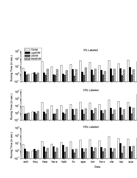
Figure 1: CPU time on the UCI data sets.

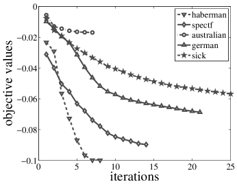
Figure 2: Number of WellSVM iterations on the UCI data sets.

5.1.2 Large-Scale Experiments

In this section, we study the scalability of the proposed WellSVM and other state-of-the-art approaches on two large data sets, real-sim and RCV1. The real-sim data has 20,958 features and 72,309 instances. while the RCV1 data has 47,236 features and 677,399 instances. The linear kernel is used. The S³VMs compared in Section 5.1.1 are for general kernels and cannot converge in 24 hours. Hence, to conduct a fair comparison, an efficient linear S³VM solver, namely, SVMlin using deterministic annealing (Sindhwani and Keerthi, 2006), is employed. All the parameters are determined in the same manner as in Section 5.1.1.

In the first experiment, we study the performance at different numbers of unlabeled examples. Specifically, $1\%,2\%,5\%,15\%,35\%,55\%$ and $75\%$ of the data (with $50$ of them labeled) are used for training, and $25\%$ of the data are for testing. This is repeated $10$ times and the average performance is reported.

Figure 3 shows the results. As can be seen, WellSVM is always superior to SVMlin, and achieves highly competitive or even better accuracy than the SVM as the number of unlabeled examples increases. Moreover, WellSVM is much faster than SVMlin. As the number of unlabeled examples increases, the difference becomes more prominent. This is mainly because SVMlin employs gradient descent while WellSVM (which is based on LIBLINEAR (Hsieh et al., 2008)) uses coordinate descent, which is known to be one of the fastest solvers for large-scale linear SVMs (Shalev-Shwartz et al., 2007).

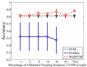
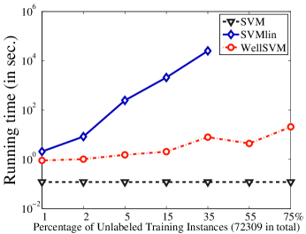
Figure 3: Semi-supervised learning results on the real-sim data with different amounts of unlabeled examples.

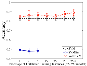
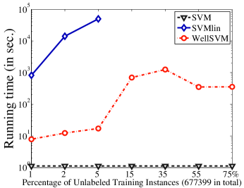
Figure 4: Semi-supervised learning results on the RCV1 data with different number of unlabeled examples.

# of labeled examples		25	50	100	150	200
real-sim	SVM	0.78 $\pm$ 0.03	0.81 $\pm$ 0.02	0.84 $\pm$ 0.02	0.86 $\pm$ 0.01	0.88 $\pm$ 0.01
	WellSVM	0.81 $\pm$ 0.08	0.84 $\pm$ 0.02	0.89 $\pm$ 0.01	0.9 $\pm$ 0.01	0.91 $\pm$ 0.01
rcv1	SVM	0.77 $\pm$ 0.03	0.83 $\pm$ 0.01	0.87 $\pm$ 0.01	0.89 $\pm$ 0.01	0.9 $\pm$ 0.01
	WellSVM	0.83 $\pm$ 0.03	0.9 $\pm$ 0.02	0.91 $\pm$ 0.01	0.92 $\pm$ 0.01	0.93 $\pm$ 0.01

Table 5: Accuracy (with standard derivations) on the real-sim and rcv1 data sets, with different numbers of labeled examples. Results for which the performance of WellSVM is significantly better than SVM are in bold.

Figure 4 shows the results on the larger RCV1 data set. As can be seen, WellSVM obtains good accuracy at different numbers of unlabeled examples. More importantly, WellSVM scales well on RCV1. For example, WellSVM takes fewer than 1,000 seconds with more than 500,000 instances. On the other hand, SVMlin cannot converge in $24$ hours when more than $5\%$ examples are used for training.

Our next experiment studies how the performance of WellSVM changes with different numbers of labeled examples. Following the setup in Section 5.1.1, $75\%$ of the examples are used for training while the rest are for testing. Different numbers (namely, 25,50,100,150, and 200) of labeled examples are randomly chosen. Since SVMlin cannot handle such a large training set, the SVM is used instead. The above process is repeated $30$ times. Table 5 shows the average testing accuracy. As can be seen, WellSVM is significantly better than SVM in all cases. The high standard deviation of WellSVM on real-sim with 25 labeled examples may be due to the fact that the large amount of unlabeled instances lead to a large variance in deriving a large margin classifier, whereas the amount of labeled examples is too small to reduce the variance.

5.1.3 Comparison with Other Benchmarks in the Literature

In this section, we further evaluate the proposed WellSVM with other published results in the literature. First, we experiment on the benchmark data sets in Chapelle et al. (2006b) by using their same setup. Results on the average test error are shown in Table 6. As can be seen, WellSVM is highly competitive.

	g241c	g241d	Digit1	USPS	COIL	BCI	Text
SVM	47.32	46.66	30.60	20.03	68.36	49.85	45.37
TSVM	24.71	50.08	17.77	25.20	67.50	49.15	40.37
WellSVM	37.37	43.33	16.94	22.74	70.73	48.50	33.70

Table 6: Test errors (%) on the SSL benchmark data sets (using 10 labeled examples). The SVM and TSVM results are from Table 21.9 in Chapelle et al. (2006b).

	SVM	$\nabla$$\text{S}^{3}$VM	c$\text{S}^{3}$VM	USVM	TSVM	$\nabla$DA	Newton	BB	WellSVM
2moons	35.6	65.0	49.8	66.3	68.7	30.0	33.5	0.0	33.5
g50c	8.2	8.3	8.3	8.5	8.4	6.7	7.5	-	7.6
text	14.8	5.7	5.8	8.5	8.1	6.5	14.5	-	8.7
uspst	20.7	14.1	15.6	14.9	14.5	11.0	19.2	-	14.3
coil20	32.7	23.9	23.6	23.6	21.8	18.9	24.6	-	23.0

Table 7: Test errors (%) of the WellSVM  and various $\text{S}^{3}$VM variants. Results of the $\text{S}^{3}$VMs compared are from Table 11 in Chapelle et al. (2008). BB can only be run on the 2moons data set due to its high computational cost. Note that in Chapelle et al. (2008), USVM is called CCCP and TSVM is called $\text{S}^{3}$VM^light.

Next, we compare WellSVM with the SVM and other state-of-the-art $\text{S}^{3}$VMs reported in Chapelle et al. (2008). These include

1. $\nabla$$\text{S}^{3}$VM (Chapelle and Zien, 2005), which minimizes the $\text{S}^{3}$VM objective by gradient descent;

2. Continuation $\text{S}^{3}$VM (c$\text{S}^{3}$VM) (Chapelle et al., 2006a), which first relaxes the $\text{S}^{3}$VM objective to a continuous function and then employs gradient descent;

3. USVM (Collobert et al., 2006);

4. TSVM (Joachims, 1999);

5. Deterministic annealing $\text{S}^{3}$VM with gradient minimization ($\nabla$DA) (Sindhwani et al., 2006), which is based on the global optimization heuristic of deterministic annealing;

6. Newton $\text{S}^{3}$VM (Newton) (Chapelle, 2007), which uses the second-order Newton’s method; and

7. Branch-and-bound (BB) (Chapelle et al., 2007).

Results are shown in Table 7. As can be seen, BB attains the best performance. Overall, WellSVM performs slightly worse than $\nabla$DA, but is highly competitive compared with the other $\text{S}^{3}$VM variants.

Finally, we compare WellSVM with MMC (Xu et al., 2005), a SDP-based S³VM, on the data sets used there. Table 8 shows the results. Again, WellSVM is highly competitive.

	HWD 1-7	HWD 2-3	Australian	Flare	Vote	Diabetes
MMC	3.2	4.7	32.0	34.0	14.0	35.6
WellSVM	2.7	5.3	40.0	28.9	11.6	41.3

Table 8: Test errors (%) of WellSVM and MMC (a SDP-based S³VM) on the data sets used in Xu et al. (2005). The MMC results are copied from their Table 2.

5.2 Multi-Instance Learning for Locating ROIs

In this section, we evaluate the proposed method on multi-instance learning, with application to ROI-location in CBIR image data. We employ the image database in Zhou et al. (2005), which consists of 500 COREL images from five image categories: castle, firework, mountain, sunset and waterfall. Each image is of size $160\times 160$, and is converted to the multi-instance feature representation by the bag generator SBN (Maron and Ratan, 1998). Each region (instance) in the image (bag) is of size 20 $\times$ 20. Some of these regions are labeled manually as ROIs. A summary of the data set is shown in Table 9. It is very labor-expensive to collect large image data with all the regions labeled. Hence, we will leave the experiments on large-scale data sets as a future direction.

concept	#images	average #ROIs per image
castle	100	19.39
firework	100	27.23
mountain	100	24.93
sunset	100	2.32
waterfall	100	13.89

Table 9: Some statistics of the image data set.

The one-vs-rest strategy is used. Specifically, a training set of 50 images is created by randomly sampling 10 images from each of the five categories. The remaining 450 images constitute the test set. This training/test split is randomly generated 10 times, and the average performance is reported.

Although many multi-instance methods have been proposed, they mainly focus on improving the classification performance, whereas only some of them are used to identify the ROIs. We list these state-of-the-art methods (Andrews et al., 2003; Maron and Ratan, 1998; Zhang and Goldman, 2002; Zhou et al., 2005) as well as related SVM-based methods for comparisons in experiments. Specifically, the WellSVM is compared with the following SVM variants: 1) MI-SVM (Andrews et al., 2003); 2) mi-SVM (Andrews et al., 2003); and 3) SVM with multi-instance kernel (MI-Kernel) (Gärtner et al., 2002). The Gaussian kernel is used for all the SVMs, where its width $\sigma$ is picked from $\{0.25\sqrt{\gamma},0.5\sqrt{\gamma},\sqrt{\gamma},2\sqrt{\gamma},4\sqrt{\gamma}\}$ with $\gamma$ being the average distance between instances; $C_{1}$ is picked from $\{C_{2},4C_{2},10C_{2}\}$; and $C_{2}$ is from $\{1,10,100\}$. We also compare with three state-of-art non-SVM-based methods that can locate ROIs, namely, Diverse Density (DD) (Maron and Ratan, 1998), EM-DD (Zhang and Goldman, 2002) and CkNN-ROI (Zhou et al., 2005). All the parameters are selected by ten-fold cross-validation (except for CkNN-ROI, in which its parameters are based on the best setting reported in Zhou et al. (2005)).

In each image classified as relevant by the algorithm, the image region with the maximum prediction value is taken as its ROI. The following two measures are used in evaluating the performance of ROI location.

1. $$\text{success rate of relevant images}=\frac{\text{number of ROI successes}}{\text{number of relevant images}}.$$ (33)

   Here, for each image predicted as relevant by the algorithm, the ROI returned by the algorithm is counted as a success if it is a real ROI.

2. The ROI success rate computed based on those images that are predicted as relevant, that is,

   $$\text{success rate of ROIs}=\frac{\text{number of ROI successes}}{\text{number of images predicted as relevant}}.$$ (34)

Notice that there is a tradeoff between these two measures. When an algorithm classifies many images as relevant, the success rate of relevant images (Equation (33)) is high while the success rate of ROIs (Equation (34)) can be low, since there are many relevant images predicted by the algorithm. On the other hand, when an algorithm classifies many images as irrelevant, the success rate of ROIs is high while the success rate of relevant images is low since many relevant images are missing. To compromise these two goals, we introduce a novel success rate of ROIs

$$\textit{success rate}=\frac{2\#\text{ROI successes}}{\#\text{relevant images}+\#\text{predicted relevant images}}.$$

This is similar to the F-score in information retrieval as

$$\frac{1}{\textit{success rate}} = \frac{\#\text{relevant images}+\#\text{predicted relevant images}}{2\#\text{ROI successes}}$$

$$= \frac{1}{2}\left(\frac{1}{\frac{\#\text{ROI successes}}{\#\text{relevant images}}}+\frac{1}{\frac{\#\text{ROI successes}}{\#\text{predicted relevant images}}}\right).$$

Intuitively, when an algorithm correctly recognizes all the relevant images and their ROIs, the success rate will be high.

Table 10 shows the success rates (with standard deviations) of the various methods. As can be seen, WellSVM achieves the best performance among all the SVM-based methods. As for its performance comparison with the other non-SVM methods, WellSVM is still always better than DD and C$k$NN-ROI, and is highly comparable to EM-DD. In particular, EM-DD achieves the best performance on castle and sunset, while WellSVM achieves the best performance on the remaining three categories (firework, mountain and waterfall). Figure 5 shows some example images with the located ROIs. It can be observed that WellSVM can correctly identify more ROIs than the other SVM-based methods.

	method	castle	firework	mountain	sunset	waterfall
	WellSVM	0.57 $\pm$ 0.12	0.68 $\pm$ 0.17	0.59 $\pm$ 0.10	0.32 $\pm$ 0.07	0.39 $\pm$ 0.13
SVM	mi-SVM	0.51 $\pm$ 0.04	0.56 $\pm$ 0.07	0.18 $\pm$ 0.09	0.32 $\pm$ 0.01	0.37 $\pm$ 0.08
methods	MI-SVM	0.52 $\pm$ 0.22	0.63 $\pm$ 0.26	0.18 $\pm$ 0.13	0.29 $\pm$ 0.10	0.06 $\pm$ 0.02
	MI-Kernel	0.56 $\pm$ 0.08	0.57 $\pm$ 0.11	0.23 $\pm$ 0.20	0.24 $\pm$ 0.03	0.20 $\pm$ 0.11
	DD	0.24 $\pm$ 0.16	0.15 $\pm$ 0.28	0.56 $\pm$ 0.11	0.30 $\pm$ 0.18	0.26 $\pm$ 0.24
non-SVM	EM-DD	0.69 $\pm$ 0.06	0.65 $\pm$ 0.24	0.54 $\pm$ 0.18	0.36 $\pm$ 0.15	0.30 $\pm$ 0.12
methods	CkNN-ROI	0.48 $\pm$ 0.05	0.65 $\pm$ 0.09	0.47 $\pm$ 0.06	0.31 $\pm$ 0.04	0.20 $\pm$ 0.05

Table 10: Success rate in locating the ROIs. The best performance and those which are comparable to the best performance (paired $t$-test at $95\%$ significance level) on each data set are bolded.

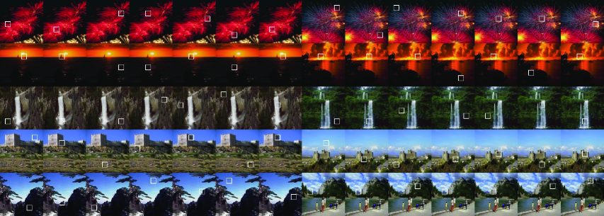
Figure 5: ROIs located by (from left to right) DD, EM-DD, CkNN-ROI, MI-SVM, mi-SVM, MI-Kernel, and WellSVM. Each row shows one category (top to bottom: firework, sunset, waterfall, castle and mountain).

5.3 Clustering

In this section, we further evaluate our WellSVM on clustering problems where all the labels are unknown. As in semi-supervised learning, 16 UCI data sets and 2 large data sets are used for comparison.

5.3.1 Small-Scale Experiments

The WellSVM is compared with the following methods: 1) $k$-means clustering (KM); 2) kernel $k$-means clustering (KKM); 3) normalized cut (NC) (Shi and Malik, 2000); 4) GMMC (Valizadegan and Jin, 2007); 5) IterSVR (Zhang et al., 2007); and 6) CPMMC (Zhao et al., 2008). In the preliminary experiment, we also compared with the original SDP-based approach in Xu et al. (2005). However, similar to the experimental results in semi-supervised learning, it does not converge after $3$ hours on the smallest data set echocardiogram. Hence, GMMC, which is also based on SDP but about 100 times faster than Xu et al. (2005), is used in the comparison.

For GMMC, IterSVR, CPMMC and WellSVM, the $C$ parameter is selected in a range $\{0.1,0.5,1,5,10,100\}$. For the UCI data sets, both the linear and Gaussian kernels are used. In particular, the width $\sigma$ of the Gaussian kernel is picked from $\{0.25\sqrt{\gamma},0.5\sqrt{\gamma},\sqrt{\gamma},$ $2\sqrt{\gamma},4\sqrt{\gamma}\}$, where $\gamma$ is the average distance between instances. The parameter of normalized cut is chosen from the same range of $\sigma$. Since $k$-means and IterSVR are susceptible to the problem of local minimum, these two methods are run 10 times and the average performance reported. We set the balance constraint in the same manner as in Zhang et al. (2007), that is, $\beta$ is set as $0.03N$ for balanced data and $0.3N$ for imbalanced data. To initialize WellSVM, 20 random label assignments are generated and the one with the maximum kernel alignment (Cristianini et al., 2002) is chosen. We also use this to initialize KM, KKM and IterSVR, and the resultant variants are denoted KM-r, KKM-r and IterSVR-r, respectively. All the methods are reported with the best parameter setting.

We follow the strategy in Xu et al. (2005) to evaluate the clustering accuracy. We first remove the labels for all instances, and then obtain the clusters by the various clustering algorithms. Finally, the misclassification error is measured w.r.t. the true labels.

We first study the clustering accuracy on 16 UCI data sets that cover a wide range of properties. Results are shown in Table 11. As can be seen, WellSVM outperforms existing clustering approaches on most data sets. Specifically, WellSVM obtains the best performance on 10 out of 16 data sets. GMMC is not as good as WellSVM. This may due to that the convex relaxation proposed in GMMC is not the same as the original SDP-based approach (Xu et al., 2005) and WellSVM.

							Iter	Iter	CP	Well
Data	KM	KM-r	KKM	KKM-r	NC	GMMC	SVR	SVR-r	MMC	SVM
Echocardiogram	0.76	0.76	0.76	0.77	0.76	0.7	0.74	0.78	0.82	0.84
House	0.89	0.89	0.89	0.88	0.89	0.78	0.87	0.87	0.53	0.90
Heart	0.66	0.59	0.69	0.59	0.57	0.7	0.59	0.59	0.56	0.59
Heart-statlog	0.68	0.79	0.78	0.79	0.79	0.77	0.76	0.76	0.56	0.81
Haberman	0.6	0.59	0.69	0.64	0.7	0.6	0.62	0.57	0.74	0.74
LiverDisorders	0.55	0.54	0.56	0.56	0.57	0.55	0.53	0.51	0.58	0.58
Spectf	0.58	0.57	0.77	0.77	0.63	0.64	0.53	0.53	0.73	0.73
Ionosphere	0.7	0.71	0.73	0.74	0.7	0.73	0.71	0.65	0.64	0.72
House-votes	0.87	0.87	0.87	0.87	0.86	0.6	0.83	0.82	0.61	0.87
Clean1	0.54	0.54	0.59	0.62	0.52	0.66	0.61	0.53	0.56	0.55
Isolet	0.98	0.96	0.89	0.95	0.98	0.56	1.00	1.00	0.5	0.98
Australian	0.54	0.55	0.57	0.57	0.56	0.6	0.56	0.51	0.56	0.83
Diabetes	0.67	0.67	0.69	0.69	0.66	0.69	0.66	0.66	0.65	0.69
German	0.57	0.56	0.68	0.62	0.66	0.56	0.56	0.64	0.7	0.7
Krvskp	0.52	0.51	0.55	0.55	0.56	-	0.51	0.51	0.52	0.54
Sick	0.68	0.63	0.88	0.77	0.84	-	0.63	0.59	0.94	0.94

Table 11: Clustering accuracies on various data sets. “-” indicates that the method does not converge in 2 hours or out-of-memory problem occurs.

The CPU time on the UCI data sets are shown in Figure 6. As can be seen, local optimization methods, such as IterSVR and CPMMC, are often efficient. As for the global optimization method, WellSVM scales much better than GMMC. On average, WellSVM is about 10 times faster. These results validate that WellSVM achieves much better scalability than the SDP-based GMMC approach. However, in general, convex methods are still slower than non-convex optimization methods on the small data sets.

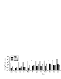
Figure 6: CPU time (in seconds) on the UCI data sets.

5.3.2 Large-Scale Experiments

In this section, we further evaluate the scalability of WellSVM on large data sets when the linear kernel is used. In this case, the WellSVM only involves solving a sequence of linear SVMs. As packages specially designed for the linear SVM (such as LIBLINEAR) are much more efficient than those designed for general kernels (such as LIBSVM), it can be expected that the linear WellSVM is also scalable on large data sets.

The real-sim data contains 72,309 instances and has 20,958 features. To study the effect of sample size on performance, different sampling rates ($1\%$, $2\%$, $5\%$ and $10\%,20\%,\ldots,100\%$) are considered. For each sampling rate (except for $100\%$), we perform random sampling 5 times, and report the average performance. Since $k$-means depends on random initialization, we run it 10 times for each sampling rate, and report its average accuracy. Figure 7 shows the accuracy and running time. As can be seen, WellSVM outperforms $k$-means and can be used on large data sets.

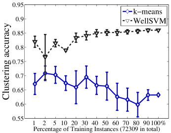
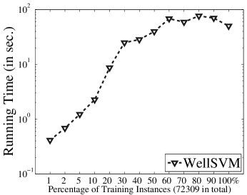
Figure 7: Clustering results on the real-sim data with different numbers of examples.

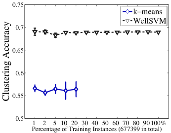
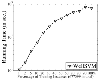
Figure 8: Clustering results on the RCV1 data with different numbers of examples.

The RCV1 data is very high-dimensional and contains more than 677,000 instances. Following the same setup as for the Real-sim data, WellSVM is compared with $k$-means under different sampling rates. Figure 8 shows the results. Note that $k$-means does not converge in 24 hours when more than 20% training instances are used. As can be seen, WellSVM obtains better performance than $k$-means and WellSVM scales quite well on RCV1. It takes fewer than 1,000 seconds for RCV1 with more than 677,000 instances and 40,000 dimensions.

6 Conclusion

Learning from weakly labeled data, where the training labels are incomplete, is generally regarded as a crucial yet challenging machine learning task. However, because of the underlying mixed integer programming problem, this limits its scalability and accuracy. To alleviate these difficulties, we proposed a convex WellSVM based on a novel “label generation” strategy. It can be shown that WellSVM is at least as tight as existing SDP relaxations, but is much more scalable. Moreover, since it can be reduced to a sequence of standard SVM training, it can directly benefit from advances in the development of efficient SVM software.

In contrast to traditional approaches that are tailored for a specific weak-label learning problem, our WellSVM formulation can be used on a general class of weak-label learning problems. Specifically, WellSVM on three common weak-label learning tasks, namely (i) semi-supervised learning where labels are partially known; (ii) multi-instance learning where labels are implicitly known; and (iii) clustering where labels are totally unknown, can all be put under the same formulation. Experimental results show that the WellSVM obtains good performance and is readily scalable on large data sets. We believe that similar conclusions can be reached on other weak-label learning tasks, such as the noisy-tolerant problem (Angluin and Laird, 1988).

The focus of this paper is on binary weakly labeled problems. For multi-class weakly labeled problems, they can be easily handled by decomposing into multiple binary problems (Crammer and Singer, 2002). However, one exception is clustering problems, in which existing decomposition methods cannot be applied as there is no label. Extension to this more challenging multi-class clustering scenario will be considered as a future work.

Acknowledgments

The authors want to thank the editor and reviewers for helpful comments and suggestions. We also thank Teng Zhang, Linli Xu and Kai Zhang for help in the experiments. This work was partially supported by the National Fundamental Research Program of China (2010CB327903), the National Science Foundation of China (61073097, 61021062), the program for outstanding PhD candidate of Nanjing University, Singapore A*star under Grant SERC 112 280 4005, and the Research Grants Council of the Hong Kong Special Administrative Region under Grant 614012. Z.-H. Zhou is the corresponding author of this paper.

A Proof of Theorem 2

Proof  Let $\{\bar{\boldsymbol{\alpha}}^{(t)},\bar{\boldsymbol{\mu}}^{(t)}\}$ be the optimal solution of Equation (9), which can be viewed as a saddle-point problem. Let $J({\boldsymbol{\alpha}},{\boldsymbol{\mu}})=\sum_{\hat{{\bf y}}\in{\cal C}^{(t)}}{\mu}_{\hat{{\bf y}}}g_{\hat{{\bf y}}}({\boldsymbol{\alpha}})$. Using the saddle-point property (Boyd and Vandenberghe, 2004), we have

$$J(\boldsymbol{\alpha},\bar{\boldsymbol{\mu}}^{(t)})\geq J(\bar{\boldsymbol{\alpha}}^{(t)},\bar{\boldsymbol{\mu}}^{(t)})\geq J(\bar{\boldsymbol{\alpha}}^{(t)},{\boldsymbol{\mu}}),\;\;\forall\boldsymbol{\alpha},\boldsymbol{\mu}.$$

In other words, $\bar{\boldsymbol{\alpha}}^{(t)}$ minimizes $J(\boldsymbol{\alpha},\bar{\boldsymbol{\mu}}^{(t)})$. Note that $g_{{{\bf y}}}(\boldsymbol{\alpha})$ is $\lambda$-strongly convex and $\sum_{{\bf y}\in{\cal C}^{(t)}}\bar{\mu}_{{\bf y}}^{(t)}=1$, thus $J({\boldsymbol{\alpha}},\bar{\boldsymbol{\mu}}^{(t)})$ is also $\lambda$-strongly convex. Using the Taylor expansion, we have

$$J({\boldsymbol{\alpha}},\bar{\boldsymbol{\mu}}^{(t)})-J(\bar{\boldsymbol{\alpha}}^{(t)},\bar{\boldsymbol{\mu}}^{(t)})\geq\frac{\lambda}{2}\|\boldsymbol{\alpha}-\bar{\boldsymbol{\alpha}}^{(t)}\|^{2},\;\;\forall\boldsymbol{\alpha}\in{\cal A}.$$

Using the definition of $J({\boldsymbol{\alpha}},{\boldsymbol{\mu}})$, we then have

$$\sum_{\hat{{\bf y}}\in{\cal C}^{(t)}}\bar{\mu}_{\hat{{\bf y}}}^{(t)}g_{\hat{{\bf y}}}(\boldsymbol{\alpha})-\sum_{\hat{{\bf y}}\in{\cal C}^{(t)}}\bar{\mu}_{\hat{{\bf y}}}^{(t)}g_{\hat{{\bf y}}}(\bar{\boldsymbol{\alpha}}^{(t)})\geq\frac{\lambda}{2}\sum_{\hat{{\bf y}}\in{\cal C}^{(t)}}\bar{\mu}_{\hat{{\bf y}}}^{(t)}\|\boldsymbol{\alpha}-\bar{\boldsymbol{\alpha}}^{(t)}\|^{2}=\frac{\lambda}{2}\|\boldsymbol{\alpha}-\bar{\boldsymbol{\alpha}}^{(t)}\|^{2}.$$ (35)

Let $\hat{{\bf y}}^{(t+1)}$ be the violated label vector selected at iteration $t+1$ in Algorithm 1, that is, ${\cal C}^{t+1}={\cal C}^{(t)}\bigcup\hat{{\bf y}}^{(t+1)}$. From the definition, we have

$$g_{\hat{{\bf y}}^{(t+1)}}(\bar{\boldsymbol{\alpha}}^{(t)})=-G(\bar{\boldsymbol{\alpha}}^{(t)},\hat{{\bf y}}^{(t+1)}) \geq \max_{\hat{{\bf y}}\in{\cal C}^{(t)}}-G(\bar{\boldsymbol{\alpha}}^{(t)},\hat{{\bf y}})+\epsilon=\max_{\hat{{\bf y}}\in{\cal C}^{(t)}}g_{\hat{{\bf y}}}(\bar{\boldsymbol{\alpha}}^{(t)})+\epsilon$$ (36)

$$\geq \sum_{\hat{{\bf y}}\in{\cal C}^{(t)}}\bar{\mu}_{\hat{{\bf y}}}^{(t)}g_{\hat{{\bf y}}}(\bar{\boldsymbol{\alpha}}^{(t)})+\epsilon=-p^{(t)}+\epsilon.$$

Consider the following optimization problem and let $\hat{p}^{(t+1)}$ be its optimal objective value

$$\hat{p}^{(t+1)}=-\min_{\boldsymbol{\alpha}\in{\cal A}}\max_{0\leq\theta\leq 1}\theta\sum_{\hat{{\bf y}}\in{\cal C}^{(t)}}\bar{\mu}_{\hat{{\bf y}}}^{(t)}g_{\hat{{\bf y}}}(\boldsymbol{\alpha})+(1-\theta)g_{\hat{{\bf y}}^{(t+1)}}(\boldsymbol{\alpha}).$$ (37)

When $\theta=1$, it reduces to Equation (9) at iteration $t$, and so $\hat{p}^{(t+1)}\leq p^{(t)}$. On the other hand, note that $\theta\sum_{\hat{{\bf y}}\in{\cal C}^{(t)}}\bar{\mu}_{\hat{{\bf y}}}^{(t)}+(1-\theta)=\theta+(1-\theta)=1$, the optimal solution in Equation (37) is suboptimal to that of Equation (9) at iteration $t+1$. Then we have $p^{(t+1)}\leq\hat{p}^{(t+1)}$. Let $\hat{p}^{(t+1)}=p^{(t)}-\eta$, now we aims at showing $\eta\geq(\frac{-c+\sqrt{c^{2}+4\epsilon}}{2})^{2}$ which obviously induces our final inequality Equation (10).

Let $\{\tilde{\boldsymbol{\alpha}}^{(t)},\tilde{\theta}\}$ be the optimal solution of Equation (37), we have following inequalities

$$p^{(t)}-\eta \leq -\sum_{\hat{{\bf y}}\in{\cal C}^{(t)}}\bar{\mu}_{\hat{{\bf y}}}^{(t)}g_{\hat{{\bf y}}}(\tilde{\boldsymbol{\alpha}}^{(t)}),$$ (38)

$$p^{(t)}-\eta \leq -g_{\hat{{\bf y}}^{(t+1)}}(\tilde{\boldsymbol{\alpha}}^{(t)}).$$ (39)

Using Equations (35), (36), (38) and (39), we have

$$\eta \geq \sum_{\hat{{\bf y}}\in{\cal C}^{(t)}}\bar{\mu}_{\hat{{\bf y}}}^{(t)}g_{\hat{{\bf y}}}(\tilde{\boldsymbol{\alpha}}^{(t)})-\sum_{\hat{{\bf y}}\in{\cal C}^{(t)}}\bar{\mu}_{\hat{{\bf y}}}^{(t)}g_{\hat{{\bf y}}}(\bar{\boldsymbol{\alpha}}^{(t)})\geq\frac{\lambda}{2}\|\tilde{\boldsymbol{\alpha}}^{(t)}-\bar{\boldsymbol{\alpha}}^{(t)}\|^{2},$$ (40)

$$\epsilon-\eta \leq g_{\hat{{\bf y}}^{(t+1)}}(\bar{\boldsymbol{\alpha}}^{(t)})-g_{\hat{{\bf y}}^{(t+1)}}(\tilde{\boldsymbol{\alpha}}^{(t)})\leq M\|\tilde{\boldsymbol{\alpha}}^{(t)}-\bar{\boldsymbol{\alpha}}^{(t)}\|.$$ (41)

On combining Equations (40) and (41), we obtain

$$\epsilon-\eta\leq M\sqrt{\frac{2\eta}{\lambda}},$$

and then finally we have ${\eta}\geq\Big{(}\frac{-c+\sqrt{c^{2}+4\epsilon}}{2}\Big{)}^{2}$, where $c=\frac{M}{\sqrt{\lambda/2}}$.

References

- Andrews et al. (2003) S. Andrews, I. Tsochantaridis, and T. Hofmann. Support vector machines for multiple-instance learning. In S. Becker, S. Thrun, and K. Obermayer, editors, Advances in Neural Information Processing Systems 15, pages 577–584. MIT Press, Cambridge, MA, 2003.
- Angluin and Laird (1988) D. Angluin and P. Laird. Learning from noisy examples. Machine Learning, 2(4):343–370, 1988.
- Bach et al. (2004) F. R. Bach, G. R. G. Lanckriet, and M. I. Jordan. Multiple kernel learning, conic duality, and the SMO algorithm. In Proceedings of the 21st International Conference on Machine Learning, pages 41–48, Banff, Canada, 2004.
- Belkin et al. (2006) M. Belkin, P. Niyogi, and V. Sindhwani. Manifold regularization: A geometric framework for learning from labeled and unlabeled examples. Journal of Machine Learning Research, 7:2399–2434, 2006.
- Boyd and Vandenberghe (2004) S. P. Boyd and L. Vandenberghe. Convex Optimization. Cambridge University Press, Cambridge, UK, 2004.
- Bucak et al. (2011) S. S. Bucak, R. Jin, and A. K. Jain. Multi-label learning with incomplete class assignments. In Proceedings of International Conference on Computer Vision and Pattern Recognition, pages 2801–2808, Colorado Springs, CO, 2011.
- Chapelle (2007) O. Chapelle. Training a support vector machine in the primal. Neural Computation, 19(5):1155–1178, 2007.
- Chapelle and Zien (2005) O. Chapelle and A. Zien. Semi-supervised classification by low density separation. In Proceedings of the 10th International Workshop on Artificial Intelligence and Statistics, The Savannah Hotel, Barbados, 2005.
- Chapelle et al. (2006a) O. Chapelle, M. Chi, and A. Zien. A continuation method for semi-supervised SVMs. In Proceedings of the 23rd International Conference on Machine Learning, pages 185–192, Pittsburgh, PA, 2006a.
- Chapelle et al. (2006b) O. Chapelle, B. Schölkopf, and A. Zien. Semi-Supervised Learning. MIT Press, Cambridge, MA, USA, 2006b.
- Chapelle et al. (2007) O. Chapelle, V. Sindhwani, and S. S. Keerthi. Branch and bound for semi-supervised support vector machines. In B. Schölkopf, J. Platt, and T. Hoffman, editors, Advances in Neural Information Processing Systems 19, pages 217–224. MIT Press, Cambridge, MA, 2007.
- Chapelle et al. (2008) O. Chapelle, V. Sindhwani, and S. S. Keerthi. Optimization techniques for semi-supervised support vector machines. Journal of Machine Learning Research, 9:203–233, 2008.
- Cheung and Kwok (2006) P. M. Cheung and J. T. Kwok. A regularization framework for multiple-instance learning. In Proceedings of the 23th International Conference on Machine Learning, pages 193–200, Pittsburgh, PA, USA, 2006.
- Collobert et al. (2006) R. Collobert, F. Sinz, J. Weston, and L. Bottou. Large scale transductive SVMs. Journal of Machine Learning Research, 7:1687–1712, 2006.
- Crammer and Singer (2002) K. Crammer and Y. Singer. On the algorithmic implementation of multiclass kernel-based vector machines. Journal of Machine Learning Research, 2:265–292, 2002.
- Cristianini et al. (2002) N. Cristianini, J. Shawe-Taylor, A. Elisseeff, and J. Kandola. On kernel-target alignment. In T. G. Dietterich, Z. Becker, and Z. Ghahramani, editors, Advances in Neural Information Processing Systems 14, pages 367–373. MIT Press, Cambridge, MA, 2002.
- De Bie and Cristianini (2006) T. De Bie and N. Cristianini. Semi-supervised learning using semi-definite programming. In O. Chapelle, B. Schölkopf, and A. Zien, editors, Semi-Supervised Learning. MIT Press, Cambridge, MA, 2006.
- Demsar (2006) Janez Demsar. Statistical comparisons of classifiers over multiple data sets. Journal of Machine Learning Research, 7:1–30, 2006.
- Dietterich et al. (1997) T. G. Dietterich, R. H. Lathrop, and T. Lozano-Pérez. Solving the multiple instance problem with axis-parallel rectangles. Artificial Intelligence, 89(1-2):31–71, 1997.
- Fan et al. (2005) R.E. Fan, P.H. Chen, and C.J. Lin. Working set selection using second order information for training support vector machines. Journal of Machine Learning Research, 6:1889–1918, 2005.
- Gärtner et al. (2002) T. Gärtner, P. A. Flach, A. Kowalczyk, and A. J. Smola. Multi-instance kernels. In Proceedings of the 19th International Conference on Machine Learning, pages 179–186, Sydney, Australia, 2002.
- Guo (2009) Y. Guo. Max-margin multiple-instance learning via semidefinite programming. In Proceedings of the 1st Asian Conference on Machine Learning, pages 98–108, Nanjing, China, 2009.
- Horst and Thoai (1999) R. Horst and N.V. Thoai. DC programming: Overview. Journal of Optimization Theory and Applications, 103(1):1–43, 1999.
- Hsieh et al. (2008) C. J. Hsieh, K. W. Chang, C. J. Lin, S. S. Keerthi, and S. Sundararajan. A dual coordinate descent method for large-scale linear SVM. In Proceedings of the 25th International Conference on Machine Learning, pages 408–415, Helsinki, Finland, 2008.
- Jain and Dubes (1988) A. K. Jain and R. C. Dubes. Algorithms for Clustering Data. Prentice Hall, Upper Saddle River, NJ, USA, 1988.
- Joachims (1999) T. Joachims. Transductive inference for text classification using support vector machines. In Proceedings of the 16th International Conference on Machine Learning, pages 200–209, Bled, Slovenia, 1999.
- Joachims (2006) T. Joachims. Training linear SVMs in linear time. In Proceedings of the 12th International Conference on Knowledge Discovery and Data mining, pages 217–226, Philadelphia, PA, 2006.
- Kelley (1960) J. E. Kelley. The cutting plane method for solving convex programs. Journal of the Society for Industrial and Applied Mathematics, 8(4):703–712, 1960.
- Kim and Boyd (2008) S.-J. Kim and S. Boyd. A minimax theorem with applications to machine learning, signal processing, and finance. SIAM Journal on Optimization, 19(3):1344–1367, 2008.
- Kloft et al. (2009) M. Kloft, U. Brefeld, S. Sonnenburg, P. Laskov, K.-R. Müller, and A. Zien. Efficient and accurate lp-norm multiple kernel learning. In Y. Bengio, D. Schuurmans, J. Lafferty, C. K. I. Williams, and A. Culotta, editors, Advances in Neural Information Processing Systems 22, pages 997–1005. MIT Press, Cambridge, MA, 2009.
- Lanckriet et al. (2004) G. R. G. Lanckriet, N. Cristianini, P. Bartlett, L. El Ghaoui, and M. I. Jordan. Learning the kernel matrix with semidefinite programming. Journal of Machine Learning Research, 5:27–72, 2004.
- Li and Zhou (2011) Y.-F. Li and Z.-H. Zhou. Towards making unlabeled data never hurt. In Proceedings of the 28th International Conference on Machine learning, pages 1081–1088, Bellevue, WA, 2011.
- Li et al. (2009a) Y.-F. Li, J.T. Kwok, I.W. Tsang, and Z.-H. Zhou. A convex method for locating regions of interest with multi-instance learning. In Proceedings of the 20th European Conference on Machine Learning and Knowledge Discovery in Databases, pages 15–30, Bled, Slovenia, 2009a.
- Li et al. (2009b) Y.-F. Li, J.T. Kwok, and Z.-H. Zhou. Semi-supervised learning using label mean. In Proceedings of the 26th International Conference on Machine Learning, pages 633–640, Montreal, Canada, 2009b.
- Li et al. (2009c) Y.-F. Li, I.W. Tsang, J.T. Kwok, and Z.-H. Zhou. Tighter and convex maximum margin clustering. In Proceedings of the 12th International Conference on Artificial Intelligence and Statistics, pages 344–351, Clearwater Beach, FL, 2009c.
- Li et al. (2012) Y.-F. Li, J.-H. Hu, Y. Jiang, and Z.-H. Zhou. Towards discovering what patterns trigger what labels. In Proceedings of the 26th AAAI Conference on Artificial Intelligence, pages 1012–1018, Toronto, Canada, 2012.
- Lobo et al. (1998) M.S. Lobo, L. Vandenberghe, S. Boyd, and H. Lebret. Applications of second-order cone programming. Linear algebra and its applications, 284(1):193–228, 1998.
- Maron and Ratan (1998) O. Maron and A. L. Ratan. Multiple-instance learning for natural scene classification. In Proceedings of the 15th International Conference on Machine Learning, pages 341–349, Madison, WI, 1998.
- Mitchell (2006) T.M. Mitchell. The discipline of machine learning. Technical report, Machine Learning Department, Carnegie Mellon University, 2006.
- Nesterov and Nemirovskii (1987) Y. Nesterov and A. Nemirovskii. Interior-Point Polynomial Algorithms in Convex Programming, volume 13. Society for Industrial Mathematics, 1987.
- Platt (1999) J. C. Platt. Fast training of support vector machines using sequential minimal optimization. In Advances in Kernel Methods - Support Vector Learning, pages 185–208. MIT Press, Cambridge, MA, USA, 1999.
- Rakotomamonjy et al. (2008) A. Rakotomamonjy, F. R. Bach, S. Canu, and Y. Grandvalet. SimpleMKL. Journal of Machine Learning Research, 9:2491–2521, 2008.
- Schölkopf and Smola (2002) B. Schölkopf and A.J. Smola. Learning with Kernels. MIT Press, 2002.
- Shalev-Shwartz et al. (2007) S. Shalev-Shwartz, Y. Singer, and N. Srebro. Pegasos: Primal estimated sub-gradient solver for svm. In Proceedings of the 24th International Conference on Machine Learning, pages 807–814, Corvallis, OR, 2007.
- Sheng et al. (2008) V.S. Sheng, F. Provost, and P.G. Ipeirotis. Get another label? improving data quality and data mining using multiple, noisy labelers. In Proceedings of the 14th International Conference on Knowledge Discovery and Data mining, pages 614–622, Las Vegas, NV, 2008.
- Shi and Malik (2000) J. Shi and J. Malik. Normalized cuts and image segmentation. IEEE Transactions on Pattern Analysis and Machine Intelligence, 22(8):888–905, 2000.
- Sindhwani and Keerthi (2006) V. Sindhwani and S.S. Keerthi. Large scale semi-supervised linear SVMs. In Proceedings of the 29th annual International Conference on Research and Development in Information Retrieval, pages 477–484, Seattle, WA, 2006.
- Sindhwani et al. (2006) V. Sindhwani, S.S. Keerthi, and O. Chapelle. Deterministic annealing for semi-supervised kernel machines. In Proceedings of the 23rd International Conference on Machine Learning, pages 841–848, Pittsburgh, PA, 2006.
- Sonnenburg et al. (2006) S. Sonnenburg, G. Rätsch, C. Schäfer, and B. Schölkopf. Large scale multiple kernel learning. Journal of Machine Learning Research, 7:1531–1565, 2006.
- Subramanya and Bilmes (2009) A. Subramanya and J. Bilmes. Entropic graph regularization in non-parametric semi-supervised classification. In Y. Bengio, D. Schuurmans, J. Lafferty, C. K. I. Williams, and A. Culotta, editors, Advances in Neural Information Processing Systems 22, pages 1803–1811. MIT Press, Cambridge, MA, 2009.
- Sun et al. (2010) Y.-Y. Sun, Y. Zhang, and Z.-H. Zhou. Multi-label learning with weak label. In Proceedings of the 24th AAAI Conference on Artificial Intelligence, pages 593–598, Atlanta, GA, 2010.
- Tsang et al. (2006) I. W. Tsang, J. T. Kwok, and P. Cheung. Core vector machines: Fast SVM training on very large data sets. Journal of Machine Learning Research, 6:363–392, 2006.
- Tsochantaridis et al. (2006) I. Tsochantaridis, T. Joachims, T. Hofmann, and Y. Altun. Large margin methods for structured and interdependent output variables. Journal of Machine Learning Research, 6(2):1453, 2006.
- Valizadegan and Jin (2007) H. Valizadegan and R. Jin. Generalized maximum margin clustering and unsupervised kernel learning. In B. Schölkopf, J. Platt, and T. Hoffman, editors, Advances in Neural Information Processing Systems 19, pages 1417–1424. MIT Press, Cambridge, MA, 2007.
- Vapnik (1998) V.N. Vapnik. Statistical Learning Theory. Wiley-Interscience, 1998.
- Wang et al. (2008) H. Y. Wang, Q. Yang, and H. Zha. Adaptive p-posterior mixture-model kernels for multiple instance learning. In Proceedings of the 25th International Conference on Machine Learning, pages 1136–1143, Helsinki, Finland, 2008.
- Xu and Schuurmans (2005) L. Xu and D. Schuurmans. Unsupervised and semi-supervised multi-class support vector machines. In Proceedings of the 20th National Conference on Artificial Intelligence, pages 904–910, Pittsburgh, PA, 2005.
- Xu et al. (2005) L. Xu, J. Neufeld, B. Larson, and D. Schuurmans. Maximum margin clustering. In L. K. Saul, Y. Weiss, and L. Bottou, editors, Advances in Neural Information Processing Systems 17, pages 1537–1544. MIT Press, Cambridge, MA, 2005.
- Xu and Frank (2004) X. Xu and E. Frank. Logistic regression and boosting for labeled bags of instances. In Proceedings of the 8th Pacific-Asia Conference on Knowledge Discovery and Data Mining, pages 272–281, Sydney, Australia, 2004.
- Xu et al. (2009) Z. Xu, R. Jin, I. King, and M. R. Lyu. An extended level method for efficient multiple kernel learning. In D. Koller, D. Schuurmans, Y. Bengio, and L. Bottou, editors, Advances in Neural Information Processing Systems 21, pages 1825–1832. MIT Press, Cambridge, MA, 2009.
- Xu et al. (2010) Z. Xu, R. Jin, H. Yang, I. King, and M. Lyu. Simple and efficient multiple kernel learning by group lasso. In Proceedings of 27th International Conference on Machine Learning, pages 1–8, Haifa, Israel, 2010.
- Yang et al. (2013) S.-J. Yang, Y. Jiang, and Z.-H. Zhou. Multi-instance multi-label learning with weak label. In Proceedings of 23rd International Joint Conference on Artificial Intelligence, Beijing, China, 2013.
- Zhang et al. (2007) K. Zhang, I. W. Tsang, and J. T. Kwok. Maximum margin clustering made practical. In Proceedings of the 24th International Conference on Machine learning, pages 1119–1126, Corvallis, OR, 2007.
- Zhang et al. (2009a) K. Zhang, J.T. Kwok, and B. Parvin. Prototype vector machine for large scale semi-supervised learning. In Proceedings of the 26th International Conference on Machine Learning, pages 1233–1240, Montreal, Canada, 2009a.
- Zhang et al. (2009b) K. Zhang, I. W. Tsang, and J. T. Kwok. Maximum margin clustering made practical. IEEE Transactions on Neural Networks, 20(4):583–596, 2009b.
- Zhang and Goldman (2002) Q. Zhang and S. A. Goldman. EM-DD: An improved multiple-instance learning technique. In T. G. Dietterich, S. Becker, and Z. Ghahramani, editors, Advances in Neural Information Processing Systems 14, pages 1073–1080. MIT Press, Cambridge, MA, 2002.
- Zhao et al. (2008) B. Zhao, F. Wang, and C. Zhang. Efficient maximum margin clustering via cutting plane algorithm. In Proceedings of the 8th International Conference on Data Mining, pages 751–762, Atlanta, GA, 2008.
- Zhou and Li (2010) Z.-H. Zhou and M. Li. Semi-supervised learning by disagreement. Knowledge and Information Systems, 24(3):415–439, 2010.
- Zhou and Xu (2007) Z.-H. Zhou and J.-M. Xu. On the relation between multi-instance learning and semi-supervised learning. In Proceedings of the 24th International Conference on Machine Learning, pages 1167–1174, Corvallis, OR, 2007.
- Zhou and Zhang (2007) Z.-H. Zhou and M.-L. Zhang. Multi-instance multi-label learning with application to scene classification. In B. Schölkopf, J. Platt, and T. Hofmann, editors, Advances in Neural Information Processing Systems 19, pages 1609–1616. MIT Press, Cambridge, MA, 2007.
- Zhou et al. (2005) Z.-H. Zhou, X.-B. Xue, and Y. Jiang. Locating regions of interest in CBIR with multi-instance learning techniques. In Proceedings of the 18th Australian Joint Conference on Artificial Intelligence, pages 92–101, Sydney, Australia, 2005.
- Zhou et al. (2012) Z.-H. Zhou, M.-L. Zhang, S.-J. Huang, and Y.-F. Li. Multi-instance multi-label learning. Artificial Intelligence, 176(1):2291–2320, 2012.
- Zhu (2006) X. Zhu. Semi-supervised learning literature survey. Technical report, Computer Science, University of Wisconsin-Madison, 2006.