Leading-order nucleon self-energy in relativistic chiral effective field theory

Abstract

We apply thermal field theory methods to compute microscopically the nucleon self-energy arising from one-pion exchange in isospin-symmetric nuclear matter and neutron matter. A self-consistent numerical scheme is introduced and its convergence is demonstrated. The repulsive contribution from the Fock exchange diagram to the energy per nucleon in symmetric nuclear matter is obtained.

I Introduction

The equation of state of bulk nuclear matter has attracted considerable attention over time, as it has a substantial impact on the properties of neutron stars as well as finite nuclei. The equation of state is determined by two, generally related, ingredients: the force between nucleons and the many-body approximation used to compute the thermodynamic properties of nuclear matter. Nuclear interactions are accurately modeled in terms of potentials arising from meson exchange: on the one hand models have been used which are based on phase-shift equivalent one-boson exchange Wiringa et al. (1995); *Stoks:1994wp; *Machleidt:2000ge; *Lacombe:1980dr and, on the other hand, more recently, (multi)-pion-exchange potentials based on chiral power counting Weinberg (1990); *Weinberg:1991um; *PhysRevC.53.2086; *2011PhR...503....1M; *2009RvMP...81.1773E. The diversity of ab-initio many-body approaches includes variational Monte Carlo methods Akmal et al. (1998); *1993RvMP...65..817B; *2007PhRvL..98j2503G; *MNL2:MNL2829 and propagator methods with (medium-) renormalized soft interactions as, e.g., in non-relativistic and covariant Brueckner-type theories Day and Wiringa (1985); *PhysRevC.84.024301; *PhysRevC.84.035801; *Sedrakian:2006mq; *2011arXiv1111.0695S. Perturbative calculations of nuclear matter properties were revived with the advent of soft chiral potentials Hebeler et al. (2011); *PhysRevC.82.014314.

In this work we apply thermal field theory (TFT) methods to compute the leading-order nucleon self-energy in isospin-symmetric nuclear and neutron matter. The method has been applied in the past in the context of QED and QCD plasmas to compute the quasiparticle energies of electrons and quarks, respectively, in a thermal medium Blaizot and Ollitrault (1993); *2001PhRvD..63f5003B. In the low-energy regime of interest to us, the relevant degrees of freedom are nucleons and pions. Chiral symmetry is an (approximate) symmetry of the strong interaction. Because chiral symmetry is spontaneously broken in nature, pions emerge as (pseudo-) Goldstone bosons of the theory. The description of the strong interaction in terms of chiral Lagrangians admits certain approximation schemes in terms of power counting of small quantities Weinberg (1979); Kaplan et al. (1996), which in principle allow for a systematic order-by-order improvement of a given calculation. Below, we will combine relativistic TFT methods and the chiral Lagrangian description of nuclear interactions to address the computation of the nucleon self-energy.

Approaches similar to ours were previously developed in Refs. Fraga et al. (2004); Lutz et al. (2000); Kaiser et al. (2002a); *2002NuPhA.700..343K; *2012PrPNP..67..299W; Lacour et al. (2011); *2010JPhG...37a5106O. Fraga et al. Fraga et al. (2004) derived analytical expressions for the zero-temperature self-energy of a nucleon due to pion exchange in dilute nuclear matter to leading order in the chiral expansion. Lutz et al. Lutz et al. (2000) and Kaiser et al. Kaiser et al. (2002a); *2002NuPhA.700..343K; *2012PrPNP..67..299W (hereafter KFW) used chiral Lagrangians and expansions in small Fermi momentum to construct equations of state in the heavy-baryon limit. The saturation in Ref. Lutz et al. (2000) arises due to correlations induced by the one-pion-exchange interaction. In Ref. Kaiser et al. (2002a); *2002NuPhA.700..343K; *2012PrPNP..67..299W two-pion exchange produces nuclear binding at the three-loop level with a suitably adjusted momentum cut-off. An effective field theory of nuclear matter with nucleons and pions, which allows for both local as well as pion-mediated multi-nucleon interactions, was developed in Ref. Lacour et al. (2011); *2010JPhG...37a5106O in the heavy-baryon limit and the main trends for the energy density of symmetric nuclear and neutron matter were already reproduced at next-to-leading order in their power-counting scheme.

In applying TFT to nuclear matter in a relativistic setting, we have to maintain the covariance of the theory by using fully relativistic thermal propagators for nucleons and pions. Keeping the Lorentz symmetries intact is of advantage, in particular, for computing the scattering and radiation amplitudes with full propagators and renormalized vertices. Specifically the computation of particular electro-weak processes in nuclear and neutron matter (or transitions in nuclei), which are driven by currents with particular Lorentz symmetry are conveniently carried out in the Dirac basis.

The second goal of our work is to maintain self-consistency among the propagators and the self-energies of the theory, which means that the iterations are performed until the Schwinger-Dyson equation for the nucleons is fulfilled. If a firm perturbative expansion (with power-counting rules) exists, a self-consistent approach generates higher-order terms in every iteration, and therefore is not really necessary. Nevertheless, using the leading-order term in the chiral expansion of the Lagrangian, we will check the impact of these higher-order terms in a self-consistent solution.

This paper is structured as follows. In Sec. II we discuss the chiral Lagrangian. Section III uses TFT to compute the pion contribution to the nucleon self-energy. Our numerical method and results for the self-energy are presented in Sec. IV. Our conclusions are collected in Sec. V. We use natural units $\hbar=c=k_{B}=1$. Four-vectors are denoted with capital letters, for instance $P^{\mu}=(p^{0},{\mathbf{p}})$.

II Lagrangians

Low-energy nuclear dynamics can be constructed on the basis of the pion and nucleon degrees of freedom starting from a chiral Lagrangian. The interaction Lagrangian ${\cal L}_{\pi N}$ between nucleons and pions is constructed such as to reflect the spontaneous chiral symmetry breaking of strong interactions at low energies. Since the interactions of Goldstone bosons must vanish at zero-momentum transfer and in the chiral limit (i.e., the pion mass $m_{\pi}\rightarrow 0$), a low-energy expansion in powers (the so-called chiral dimension) of the ratio of the momentum or the pion mass over ($4\pi$ times) the pion decay constant can be performed. Consequently, the Lagrangian can be written as

$${\cal L}_{\pi N}={\cal L}_{\pi N}^{(1)}+{\cal L}_{\pi N}^{(2)}+\ldots,$$ (1)

where the superscript labels the order of the chiral dimension. The terms in the expansion (1) are constructed by introducing the following $SU(2)$ matrix $U$ in flavor space

$$U=\exp\left(i\frac{{\bm{\tau}}\cdot{\bm{\pi}}}{f_{\pi}}\right)=1+\frac{i}{f_{\pi}}\mbox{\boldmath$\tau$}\cdot\mbox{\boldmath$\pi$}-\frac{1}{2f_{\pi}^{2}}\mbox{\boldmath$\pi$}^{2}+\ldots,$$ (2)

where ${\bm{\tau}}$ is vector of Pauli matrices in isospin space, ${\bm{\pi}}$ is the isotriplet of pions, and $f_{\pi}$ the pion decay constant. The leading-order term is given by Gasser and Leutwyler (1988)

$${\cal L}^{(1)}_{\pi N}=\bar{\psi}\left(i\gamma^{\mu}D_{\mu}-m+\frac{g_{A}}{2}\gamma^{\mu}\gamma_{5}u_{\mu}\right)\psi\,,$$ (3)

where $\psi$ is the nucleon field, $\bar{\psi}=\psi^{\dagger}\gamma_{0}$, $m$ is the nucleon mass, and $g_{A}$ is the axial-vector coupling. The physical value of $g_{A}$ is determined from neutron beta decay and is given by $g_{A}=1.2695\pm 0.0029$. $D_{\mu}$ is the covariant derivative,

$$D_{\mu}=\partial_{\mu}+\Gamma_{\mu}$$ (4)

where $\Gamma_{\mu}$ is the so-called chiral connection which couples an even number of pions to the nucleon and is defined as

$$\Gamma_{\mu} = i\{\xi^{\dagger},\partial_{\mu}\xi\}=i(\xi^{\dagger}\partial_{\mu}\xi+\xi\partial_{\mu}\xi^{\dagger})$$ (5)

$$= -\frac{1}{4f_{\pi}^{2}}\,{\bm{\tau}}\cdot({\bm{\pi}}\times\partial_{\mu}{\bm{\pi}})+\ldots$$

with $\xi=\sqrt{U}$. The Lagrangian (3) also includes the axial-vector current $u_{\mu}$ which couples an odd number of pions to the nucleon

$$u_{\mu}=i[\xi^{\dagger},\partial_{\mu}\xi]=i(\xi^{\dagger}\partial_{\mu}\xi-\xi\partial_{\mu}\xi^{\dagger})=-\frac{1}{f_{\pi}}\,\mbox{\boldmath$\tau$}\cdot\partial_{\mu}\mbox{\boldmath$\pi$}+\ldots\;.$$ (6)

Keeping only the lowest-order term in the chiral Lagrangian (3) the pion-nucleon Lagrangian reads Machleidt and Entem (2011)

$${\cal L}_{\pi N}^{(1)}=\bar{\psi}\left(i\gamma^{\mu}\partial_{\mu}-m-\frac{g_{A}}{2f_{\pi}}\gamma^{\mu}\gamma_{5}{\bm{\tau}}\cdot\partial_{\mu}{\bm{\pi}}\right)\psi,$$ (7)

where we have neglected the Weinberg-Tomozawa contribution arising from the chiral connection (5). The chiral one-pion interaction term in Eq. (7) takes the light dynamical degrees of freedom, i.e., pions, explicitly into account. The complete interaction Lagrangian includes to lowest order an additional four-fermion contact term. Thus, the Lagrangian of the system can be written as

$${\cal L}={\cal L}_{\rm free}+{\cal L}_{\pi N}^{(1)}+{\cal L}_{NN},$$ (8)

where the first term is the Lagrangian of the non-interacting system and the last term corresponds to the four-fermion interaction. Figure 1 shows the two distinct leading-order contributions to the self-energy of a nucleon originating from the tree-level vertices in the Lagrangian (8).

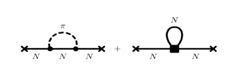
Figure 1: The diagrams contributing to the self-energy of the nucleon to lowest order. The first one represents the chiral one-pion exchange contribution to the nucleon self-energy. Solid lines refer to nucleons, dashed lines to pions and dots to pion-nucleon vertices. The second diagram is the contribution from the four-fermion contact interaction, with the square vertex representing the two-body scattering matrix.

III Pion contribution to the self-energy

III.1 Leading-order contribution

In this section we evaluate the one-pion contribution to the nucleon self-energy, corresponding to the left diagram in Fig. 1, within the imaginary-time formalism. The free covariant propagator of the nucleons in energy-momentum space is given by

$${S}_{0}(K)=\frac{\Lambda^{+}_{k}\gamma_{0}}{ik_{n}+\mu-E_{k}}+\frac{\Lambda^{-}_{k}\gamma_{0}}{ik_{n}+\mu+E_{k}},$$ (9)

where the zeroth component of the four-momentum $K^{\mu}\equiv(k^{0},{\mathbf{k}})$ takes discrete values, $k^{0}=ik_{n}=(2n+1)\pi iT$, $n\in\mathbb{Z}$ and $T$ is the temperature. $\Lambda^{\pm}_{k}$ are projectors onto positive $(+)$ and negative $(-)$ energy states,

$$\Lambda^{\pm}_{k}=\frac{1}{2E_{k}}\left[E_{k}\pm(\bm{\alpha}\cdot{{\mathbf{k}}}+m\gamma_{0})\right],$$ (10)

where $E_{k}^{2}={{\mathbf{k}}}^{2}+m^{2}$ is the dispersion relation for non-interacting nucleons, $m$ is their mass, and $\bm{\alpha}\equiv\gamma_{0}\bm{\gamma}$. The free pion propagator is given by

$$D_{0}(Q)=\frac{1}{2\omega_{q}}\left(\frac{1}{i\omega_{n}-\omega_{q}}-\frac{1}{i\omega_{n}+\omega_{q}}\right)\;,$$ (11)

where the zeroth component of the four-momentum $Q^{\mu}\equiv(q^{0},{\mathbf{q}})$ takes discrete values $q^{0}=i\omega_{n}=2n\pi iT$, $n\in\mathbb{Z}$, and $\omega_{q}^{2}=q^{2}+m_{\pi}^{2}$ is the dispersion relation for non-interacting pions, with $m_{\pi}$ being the free pion mass. In terms of the free propagators (9) and (11) the one-pion exchange contribution to the nucleon self-energy reads

$$\Sigma(P) = -\frac{3g_{A}^{2}}{4f_{\pi}^{2}}T\int\!\!\frac{d^{3}{\mathbf{k}}}{(2\pi)^{3}}\sum_{ik_{n}}D_{0}(P-K)\gamma_{5}(\not{P}-\not{K})$$ (12)

$$\times S_{0}(K)\gamma_{5}(\not{P}-\not{K})\;,$$

where $P^{\mu}=(p^{0},{\mathbf{p}})\equiv(ip_{n},{\mathbf{p}})$. We substitute the propagators (9) and (11) into Eq. (12) and carry out the summation over the fermionic Matsubara frequency $ik_{n}$. In general, this sum generates physically distinct processes involving all possible combinations of bosons and fermions and their antiparticles. The result of the summation can be arranged according to these underlying processes, but it is more convenient to separate the self-energy into the “vacuum” and “thermal” parts $\Sigma(P)=\Sigma_{0}(P)+\Sigma_{T}(P)$, where the vacuum part is given by

$$\Sigma_{0}(P) = \frac{3g_{A}^{2}}{4f_{\pi}^{2}}\int\frac{d^{3}{\mathbf{k}}}{(2\pi)^{3}}\frac{1}{2\omega_{pk}}$$ (13)

$$\times \Biggl{[}\frac{\gamma_{5}(\not{P}-\not{K})\Lambda^{+}_{k}\gamma_{0}\gamma_{5}(\not{P}-\not{K})}{ip_{n}+\mu-E_{k}-\omega_{pk}}\bigg{|}_{k_{0}=ip_{n}-\omega_{pk}}$$

$$+ \frac{\gamma_{5}(\not{P}-\not{K})\Lambda^{-}_{k}\gamma_{0}\gamma_{5}(\not{P}-\not{K})}{ip_{n}+\mu+E_{k}+\omega_{pk}}\bigg{|}_{k_{0}=E_{k}+\mu}\Biggr{]}\;,$$

and the thermal part is given by

$$\Sigma_{T}(P) = \frac{3g_{A}^{2}}{4f_{\pi}^{2}}\int\frac{d^{3}{\mathbf{k}}}{(2\pi)^{3}}\frac{1}{2\omega_{pk}}$$ (14)

$$\bigg{\{} \left[\frac{1}{ip_{n}+\mu-E_{k}-\omega_{pk}}-\frac{1}{ip_{n}+\mu-E_{k}+\omega_{pk}}\right]\gamma_{5}(\not{P}-\not{K})\Lambda^{+}_{k}\gamma_{0}\gamma_{5}(\not{P}-\not{K})\big{|}_{k_{0}=E_{k}-\mu}n_{F}(E_{k}-\mu)$$

$$- \left[\frac{1}{ip_{n}+\mu+E_{k}-\omega_{pk}}-\frac{1}{ip_{n}+\mu+E_{k}+\omega_{pk}}\right]\gamma_{5}(\not{P}-\not{K})\Lambda^{-}_{k}\gamma_{0}\gamma_{5}(\not{P}-\not{K})\big{|}_{k_{0}=-E_{k}-\mu}n_{F}(E_{k}-\mu)$$

$$- \gamma_{5}(\not{P}-\not{K})\left[\frac{\Lambda^{+}_{k}\gamma_{0}}{ip_{n}+\mu-E_{k}-\omega_{pk}}+\frac{\Lambda^{-}_{k}\gamma_{0}}{ip_{n}+\mu+E_{k}-\omega_{pk}}\right]\gamma_{5}(\not{P}-\not{K})\big{|}_{k_{0}=ip_{n}-\omega_{pk}}n_{B}(\omega_{pk})$$

$$- \gamma_{5}(\not{P}-\not{K})\left[\frac{\Lambda^{+}_{k}\gamma_{0}}{ip_{n}+\mu-E_{k}+\omega_{pk}}+\frac{\Lambda^{-}_{k}\gamma_{0}}{ip_{n}+\mu+E_{k}+\omega_{pk}}\right]\gamma_{5}(\not{P}-\not{K})\big{|}_{k_{0}=ip_{n}+\omega_{pk}}n_{B}(\omega_{pk})\bigg{\}}\;,$$

where $\omega_{pk}^{2}=({\mathbf{p}}-{\mathbf{k}})^{2}+m_{\pi}^{2}$ and $n_{F/B}(x)=[\exp(x/T)\pm 1]^{-1}$ are the Fermi/Bose distribution functions. The retarded self-energy is obtained by analytical continuation, i.e., $ip_{n}\rightarrow p_{0}+i0^{+}$. We have verified that in the case of a Yukawa interaction Eq. (14) transforms to the well-known expression for the self-energy of a fermion in finite-temperature quantum field theory Blaizot and Ollitrault (1993); Kapusta (1989).

At sufficiently low temperature the occupation number of anti-particles is so small that we can neglect their contribution in Eq. (14). Furthermore, we assume that there is no macroscopic occupation of pionic modes in nuclear matter at any temperature and density of interest; therefore, we also drop the contributions proportional to the bosonic occupation numbers. The remaining contribution arises from the pole at $k_{0}\equiv E_{k}-\mu$ and we arrive at

$$\Sigma_{T}(P) = \frac{3g_{A}^{2}}{4f_{\pi}^{2}}\int\frac{d^{3}{\mathbf{k}}}{(2\pi)^{3}}\frac{1}{2\omega_{pk}}\left[\frac{1}{p_{0}-k_{0}-\omega_{pk}+i0^{+}}-\frac{1}{p_{0}-k_{0}+\omega_{pk}+i0^{+}}\right](s+\not{Q})n_{F}(k_{0})\;,$$ (15)

where we have defined the quantities $s=-(m/2E_{k})(P-K)^{2}$ and $Q^{\mu}=(q_{0},{\mathbf{q}})$, with components

$$q_{0} = \frac{1}{2}[(p_{0}-k_{0})^{2}+({\mathbf{p}}-{\mathbf{k}})^{2}]-\frac{1}{E_{k}}({\mathbf{p}}-{\mathbf{k}})\cdot{\mathbf{k}}(p_{0}-k_{0})\;,$$ (16)

$${\mathbf{q}} = -\frac{1}{2E_{k}}\left[(P-K)^{2}{\mathbf{k}}+2({\mathbf{p}}-{\mathbf{k}})\cdot{\mathbf{k}}({\mathbf{p}}-{\mathbf{k}})\right]+(p_{0}-k_{0})({\mathbf{p}}-{\mathbf{k}})\;.$$ (17)

Later on we will enforce self-consistency in evaluating the self-energy. This requires a Lorentz decomposition of the self-energy, which in the most general case is given by

$$\Sigma(P)=\Sigma_{s}(P)+\gamma_{5}\Sigma_{ps}(P)+\gamma^{\mu}\Sigma_{\mu}(P)+\gamma_{5}\gamma^{\mu}\Sigma^{A}_{\mu}(P)+\sigma^{\mu\nu}\Sigma_{\mu\nu}(P)\;.$$ (18)

The requirements of parity conservation, translational and rotational invariance, as well as time-reversal invariance, reduce this most general decomposition to the following form

$$\Sigma(P)=\Sigma_{s}(P)+\gamma_{0}\Sigma_{0}(P)+{\mbox{\boldmath$\gamma$}}\cdot{\mathbf{p}}\Sigma_{v}(P)\;.$$ (19)

Equation (15) can now be projected onto its Lorentz components by multiplying it with $1,\gamma_{0}$, and $\bm{\gamma}$, and taking the trace over the $\gamma$-matrices. Keeping only the thermal part of the self-energy (and dropping the index $T$ on the self-energies), this leads us to the following decomposition coefficients

$$\Sigma_{s}(P) = -\frac{3g_{A}^{2}}{4f_{\pi}^{2}}\int\frac{d^{3}{\mathbf{k}}}{(2\pi)^{3}}\frac{1}{2\omega_{pk}}\left[\frac{1}{p_{0}-k_{0}-\omega_{pk}+i0^{+}}-\frac{1}{p_{0}-k_{0}+\omega_{pk}+i0^{+}}\right]n_{F}(k_{0})\frac{m}{2E_{k}}(P-K)^{2}\;,$$ (20)

$$\Sigma_{0}(P) = +\frac{3g_{A}^{2}}{4f_{\pi}^{2}}\int\frac{d^{3}{\mathbf{k}}}{(2\pi)^{3}}\frac{1}{2\omega_{pk}}\left[\frac{1}{p_{0}-k_{0}-\omega_{pk}+i0^{+}}-\frac{1}{p_{0}-k_{0}+\omega_{pk}+i0^{+}}\right]n_{F}(k_{0})$$ (21)

$$\times \left[\frac{1}{2}((p_{0}-k_{0})^{2}+({{\mathbf{p}}}-{\mathbf{k}})^{2})+\frac{1}{E_{k}}({\mathbf{p}}-{\mathbf{k}})\cdot{\mathbf{k}}(p_{0}-k_{0})\right]\;,$$

$$|{\mathbf{p}}|\Sigma_{v}(P) = +\frac{3g_{A}^{2}}{4f_{\pi}^{2}}\int\frac{d^{3}{\mathbf{k}}}{(2\pi)^{3}}\frac{1}{2\omega_{pk}}\left[\frac{1}{p_{0}-k_{0}-\omega_{pk}+i0^{+}}-\frac{1}{p_{0}-k_{0}+\omega_{pk}+i0^{+}}\right]n_{F}(k_{0})$$ (22)

$$\times \Biggl{\{}\frac{1}{2E_{k}}\left[(P-K)^{2}{\mathbf{k}}+2({\mathbf{p}}-{\mathbf{k}})\cdot{\mathbf{k}}({\mathbf{p}}-{\mathbf{k}})\right]-(p_{0}-k_{0})({\mathbf{p}}-{\mathbf{k}})\Biggr{\}}\cdot\hat{\mathbf{p}}\;,$$

where $\hat{\mathbf{p}}={\mathbf{p}}/|{\mathbf{p}}|$ is a unit vector. Equations (20)–(22) are our final result for the chiral one-pion-exchange contribution to the nucleon self-energy. It is evident that the other terms in Eq. (14), which could become important at higher temperatures and densities, can be evaluated in a completely analogous way.

III.2 Further approximations

For numerical computations the factor $s+\not{Q}$ in Eq. (15) can be simplified. We start by rewriting the expression

$$2E_{k}\not{Q} = 2E_{k}(q_{0}\gamma_{0}-{\mathbf{q}}\cdot\bm{\gamma})=\mu\left[(p_{0}-k_{0})^{2}+({\mathbf{p}}-{\mathbf{k}})^{2}\right]\gamma_{0}$$ (23)

$$+ 2(P-K)\cdot K\not{P}-(P^{2}-K^{2})\not{K}$$

$$- 2\mu(p_{0}-k_{0})({\mathbf{p}}-{\mathbf{k}})\cdot\bm{\gamma}\;.$$

For the densities and temperatures of interest, nucleons are constrained to the vicinity of their Fermi surface, therefore the momentum of the nucleon can be expressed as $\mathbf{p}=p_{F}\hat{\mathbf{n}}+\delta\mathbf{p}$. Here, $p_{F}$ is the nucleon Fermi momentum, $\hat{\mathbf{n}}$ is a unit vector, and $\delta\mathbf{p}$ is the residual momentum, with $|\delta\mathbf{p}|\ll p_{F}$. Furthermore, the relativity parameter $x=p_{F}/m$ is small as well; numerically, we have

$$x\approx 0.28\left(\frac{n}{n_{0}}\right)^{1/3}\;,$$ (24)

where $n$ is the density of the systems, $n_{0}=0.16\;{\rm fm}^{-3}$ is the nuclear saturation density. Then, the nucleon energy is $E_{p}\approx m(1+{\mathbf{p}}^{2}/2m^{2})$ and the chemical potential $\mu\approx m(1+p_{F}^{2}/2m^{2})$. This implies that $p_{0}=E_{p}-\mu\approx({\mathbf{p}}^{2}-p_{F}^{2})/2m\approx x\,\hat{\mathbf{n}}\cdot\delta\mathbf{p}$ is small compared to $|{\mathbf{p}}|\approx p_{F}$. Therefore, we can replace $(P-K)^{2}\approx-(\mathbf{p}-\mathbf{k})^{2}$.

With these approximations we obtain

$$2E_{k}~{}\not{Q} \approx 2m~{}\not{Q}\approx\mu({\mathbf{p}}-{\mathbf{k}})^{2}\gamma_{0}-2({\mathbf{p}}-{\mathbf{k}})\cdot{\mathbf{k}}\not{P}$$ (25)

$$+ ({\mathbf{p}}^{2}-{\mathbf{k}}^{2})\not{K}-({\mathbf{p}}^{2}-{\mathbf{k}}^{2})({\mathbf{p}}-{\mathbf{k}})\cdot\bm{\gamma}$$

$$\approx ({\mathbf{p}}-{\mathbf{k}})^{2}[(p_{0}+\mu)\gamma_{0}-{\mathbf{p}}\cdot\bm{\gamma}]$$

where we used the fact that $p_{0}-k_{0}\approx({\mathbf{p}}^{2}-p_{F}^{2})/2m-({\mathbf{k}}^{2}-p_{F}^{2})/2m=({\mathbf{p}}^{2}-{\mathbf{k}}^{2})/2m$.

Therefore, the factor $s+\not{Q}$ in the integrand of the self-energy (15) reads now

$$s+\not{Q}\approx\frac{(\mathbf{p}-\mathbf{k})^{2}}{2m}[m+(p_{0}+\mu)\gamma_{0}-\bm{\gamma}\cdot{\mathbf{p}}]\;.$$ (26)

Separating the contributions from particles and anti-particles in the boson propagator, with these approximations the self-energy reads

$$\Sigma(P) \approx [m+(p_{0}+\mu)\gamma_{0}-\bm{\gamma}\cdot{\mathbf{p}}]\left[\sigma_{+}(P)+\sigma_{-}(P)\right]$$ (27)

$$\equiv [m+(p_{0}+\mu)\gamma_{0}-\bm{\gamma}\cdot{\mathbf{p}}]~{}\sigma(P)\;,$$

where

$$\sigma_{\pm}(P)=\pm\frac{3g_{A}^{2}}{8mf_{\pi}^{2}}\int\frac{d^{3}{\mathbf{k}}}{(2\pi)^{3}}\frac{1}{2\omega_{pk}}\frac{(\mathbf{p}-\mathbf{k})^{2}}{p_{0}-k_{0}\mp\omega_{pk}+i\eta}n_{F}(k_{0}),$$ (28)

is the reduced self-energy. Therefore, the coefficients of the Lorentz decomposition of the self-energy can be expressed in terms of $\sigma(p)$,

$$\Sigma_{s}(P)\approx m\sigma(P),\quad\Sigma_{0}(P)\approx(p_{0}+\mu)\sigma(P),$$

$$\Sigma_{v}(P)\approx-\sigma(P)\;.$$ (29)

The real part of the self-energy can now be computed with the help of the Dirac identity. We obtain by explicitly evaluating the Cauchy principal value of Eq. (28)

$${\rm Re}[\sigma(P)] \equiv {\rm Re}[\sigma_{+}(P)+\sigma_{-}(P)]$$

$$= \frac{3g_{A}^{2}}{32m\pi^{2}f_{\pi}^{2}}\int_{0}^{\infty}\!\!\!d|{\mathbf{k}}|\,{\mathbf{k}}^{2}\,\frac{n_{F}(k_{0})}{2|{\mathbf{p}}||{\mathbf{k}}|}~{}\int_{-1}^{1}\!\!dx\frac{({\mathbf{p}}-{\mathbf{k}})^{2}}{x-x_{0}}$$

where $x_{0}=[{\mathbf{p}}^{2}+{\mathbf{k}}^{2}+m_{\pi}^{2}-(p_{0}-k_{0})^{2}]/(2|{\mathbf{p}}||{\mathbf{k}}|)$.

III.3 Enforcing self-consistency

The self-consistency of the numerical computation of the self-energy is achieved by replacing the free nucleon propagator in Eq. (12) by the full nucleon propagator, determined by the Schwinger-Dyson equation

$$S^{-1}(P) = S_{0}^{-1}(P)-\Sigma(P)=[(p_{0}+\mu)\gamma_{0}-\bm{\gamma}\cdot{\mathbf{p}}]$$

$$\times [1-{\rm Re}\sigma(P)]-m[1+{\rm Re}\sigma(P)]+{\rm Im}\Sigma(P),$$

where the free nucleon propagator is given by $S_{0}^{-1}(P)=(p_{0}+\mu)\gamma_{0}-\bm{\gamma}\cdot{\mathbf{p}}-m$ and we have used Eq. (27) for the nucleon self-energy. The roots of ${\rm det}S^{-1}(P)$ determine the excitation spectrum of the system,

$$p_{0}^{*}=E_{p}^{*}-\mu^{*}\;,$$ (32)

where

$$E_{p}^{*} = \sqrt{{{\mathbf{p}}^{*}}^{2}+{m^{*}}^{2}}\;,$$ (33)

$$m^{*} = m[1+{\rm Re}\sigma(P^{*})]\;,$$ (34)

$${\mathbf{p}}^{*} = {\mathbf{p}}[1-{\rm Re}\sigma(P^{*})]\;,$$ (35)

$$\mu^{*} = \mu[1-{\rm Re}\sigma(P^{*})]\;.$$ (36)

We achieve self-consistency for the self-energy by replacing the free quantities $m$, ${\mathbf{p}}$, ${\mathbf{k}}$, and $\mu$ in the integrand (but not in the integration measure) of Eq. (III.2) by the corresponding renormalized $m^{*}$, ${\mathbf{p}}^{*}$, ${\mathbf{k}}^{*}$, and $\mu^{*}$. In practice, we start by computing (III.2) with the free quantities, which define the renormalized quantities (33)–(36) to first order in the iteration process. We repeat the previous step until convergence is reached. Approximations made in the numerical part of this work are purely technical and concern only the computation of traces in the self-energy diagram. It is evident from Eqs. (33)–(36) that the pole structure and, therefore, the quasiparticle spectra as well as the Lorentz structure of the self-energies remains fully relativistic. During the iteration procedure the quantities in Eqs. (33)–(36) are corrected in each iteration differently according to the Lorentz structure of the self-energy and propagators. Thus the Dirac structure of the self-energies and propagators is maintained.

IV Results

We will not attempt to evaluate the contributions to the energy of nuclear matter from diagrams other than the one-pion exchange discussed in the previous section. For that purpose we define the energy per nucleon, excluding its rest mass $m$, via the formula

$$\frac{E}{N}={\cal T}+{\cal U}-m\;,$$ (37)

where ${\cal T}$ is the kinetic energy, ${\cal U}$ is the potential energy and $N$ is the particle number. In terms of the renormalized quantities (34)–(36) the kinetic energy reads

$${\cal T}=\frac{g_{\tau}}{\pi^{2}n}\int d|{\mathbf{p}}|\,{\mathbf{p}}^{2}\left(\frac{m^{*}}{E_{p}^{*}}m+\frac{|{\mathbf{p}}^{*}|}{E_{p}^{*}}|{\mathbf{p}}|\right)n_{F}(E_{p}^{*}-\mu^{*})\;,$$ (38)

where $g_{\tau}$ is the isospin degeneracy factor ($g_{\tau}=2$ in isospin-symmetric nuclear matter and $g_{\tau}=1$ in neutron matter). The potential energy ${\cal U}$ is given by

$${\cal U} = \frac{g_{\tau}}{2\pi^{2}n}\int d|{\mathbf{p}}|\,{\mathbf{p}}^{2}\left[\frac{m^{*}}{E_{p}^{*}}m+E_{p}-\frac{|{\mathbf{p}}^{*}|}{E_{p}^{*}}|{\mathbf{p}}|\right]$$ (39)

$$\times \sigma(P^{*})n_{F}(E_{p}^{*}-\mu^{*})\;.$$

As we consider only spin-unpolarized matter, the spin summation has been carried out in Eqs. (38) and (39).

IV.1 Symmetric nuclear matter

The Fock diagram evaluated in the previous section represents chiral one-pion exchange between two nucleons. Chiral power counting requires to leading order an additional two-body contact term. The corresponding self-energy diagrams are shown by the left and the right diagrams in Fig. 1. In passing we note that if in the nuclear medium the contact is density independent then its contribution is given simply by $\Sigma_{c}=t^{(2)}n,$ where $n$ is the density and $t^{(2)}$ is the two-body contact.

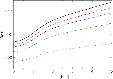
Figure 2: (Color online) Real part of the reduced nucleon self-energy as a function of momentum $p$ at $n=0.1\;{\rm fm}^{-3}$ and $T=0$. The dotted (violet) line is the lowest-order result and simultaneously the starting point of the iteration. The full (black) line represents the final self-consistent result. The other lines correspond to 2,3,4,5 (from bottom to top) iteration steps.

The reduced self-energy due to the chiral one-pion exchange in isospin-symmetric nuclear matter is shown in Fig. 2 at $T=0$ and $n=0.1\;{\rm fm}^{-3}$. As one observes, the self-consistency procedure converges rapidly. In order to achieve a relative accuracy $\leq 10^{-6}$ one needs about 10 iterations, the exact number of iteration depending on the density. For small densities the number of required iterations is small, while for large densities the number of iterations needed to achieve convergence is larger. While the self-energy does not tend to zero for large external momenta, the result for the energy of the system is convergent due to an additional integration over a Fermi distribution function. Our numerical implementation of the self-consistency shows that the perturbative expansion is not perfect and iterations are necessary (see Fig. 2). We see that chiral power counting at non-zero density and temperature is not reliable anymore, since several new scales (temperature and chemical potential) appear.

In Fig. 3 we show the reduced self-energy at zero temperature in comparison to its form at $T=20$ MeV. The change with temperature can be seen to be rather moderate. In the non-zero temperature case the self-energy is larger for low momenta than at zero temperature, while for higher momenta the variation of temperature does not affect the result very much. This is due to the fact that we deal with comparatively low temperatures, therefore the temperature is a relevant scale only at low momenta.

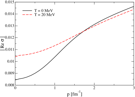
Figure 3: (Color online) Dependence of the one-pion exchange contribution to the nucleon self-energy in isospin-symmetric nuclear matter on the momentum at density $n=0.1$ fm^-3. The solid line shows the real part of the self-energy for temperature $T=0$ and the dashed line for $T=20$ MeV.

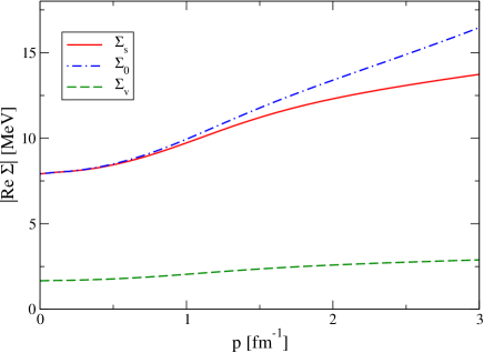
Figure 4: (Color online) The Lorentz components of the real part of the nucleon self-energy as a function of momentum $p$ at $n=0.1\;{\rm fm}^{-3}$ and $T=0$.

In Fig. 4 we show the Lorentz components of the real part of the full self-energy at $n=0.1$ fm^-3 and $T=0$. It can be seen that the vector self-energy is substantially smaller than the other contributions to the self-energy, as expected.

Our numerical calculations of the Fock contribution to the self-energy of nucleons can be validated in certain limiting cases. We verified that our numerical result for the real part of the reduced self-energy is in good agreement with the analytical result quoted in Ref. Fraga et al. (2004) at zero temperature. A further test is the comparison of the energies per particle of nuclear matter with those of KFW, where the energy per particle was computed directly without a reference to the self-energy. Their result for the zero-temperature one-pion-exchange Fock diagram, which is an expansion in the small relativity parameter $x$, reads Kaiser et al. (2002a); *2002NuPhA.700..343K; *2012PrPNP..67..299W

$$E{(T=0)}={3g_{A}^{2}p_{F}^{3}\over 16\pi^{2}f_{\pi}^{2}}\left(a_{0}+a_{2}x^{2}\right)\,,$$ (40)

where the coefficients of this expansion $a_{0}$ and $a_{2}$ are functions of the ratio $p_{F}/m_{\pi}$ alone and can be calculated analytically INSET . In Fig. 5 we show the contributions of the one-pion exchange to the energy of the matter from various Lorentz components along with the full result which is the sum of the three components. Our full result is in good agreement with the analytical expression by KFW, Eq. (40), also shown in Fig. 5.

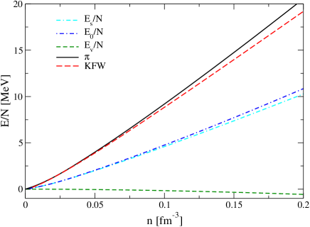
Figure 5: (Color online) Dependence of various contributions to the energy per particle on density. The full result is shown by the solid (black) line, the KFW result is shown by the dashed (red) line. The remaining lines show the energy per particle according to the contribution of various Lorentz components: the scalar component $E_{s}$ (double dash-dotted, cyan), the zero component $E_{0}$ (dash-dotted, blue) and vector component $E_{v}$ (dashed, green).

IV.2 Pure neutron matter

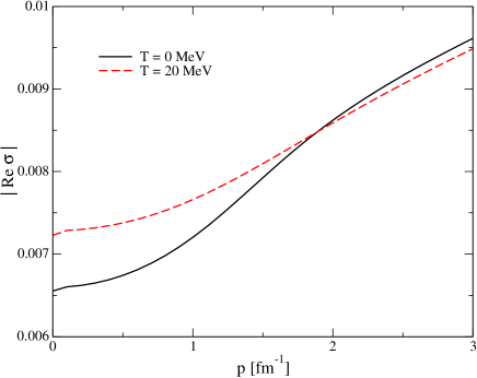
Figure 6: (Color online) Dependence of the one-pion exchange contribution to the nucleon self-energy in pure neutron matter on the momentum, at density $n=0.1$ fm^-3. The solid line shows the real part of the self-energy for temperature $T=0$ while the dashed line is for $T=20$ MeV.

The reduced self-energy of neutrons in pure neutron matter is shown in Fig. 6. Compared to isospin-symmetric nuclear matter, the self-energy in neutron matter is smaller. This is due to the fact that in pure neutron matter one-pion exchange involves only the $\pi^{0}$-meson. At non-zero temperature, as in the case of isospin-symmetric nuclear matter, we observe that, for low momenta, the contribution of the self-energy is larger, but the difference among the two cases tends to disappear with increasing momentum.

V Conclusions

In this work we have combined the methods of TFT and chiral Lagrangians to compute the self-energy of nucleons to leading order in the chiral expansion. In doing so, we have maintained the covariance of the pion and nucleon propagators and we have imposed self-consistency by solving a Schwinger-Dyson equation for the nucleon self-energy. Our approach has also been applied to pure neutron matter, with similar results.

Clearly, to obtain a consistent phenomenology of both isospin-symmetric nuclear and pure neutron matter, one needs to introduce contact interactions which account for the short-range two-body and three-body interactions. Furthermore, the importance of second-order pion exchange was already stressed by Lutz et al. Lutz et al. (2000) and KFW. In this respect further steps might be undertaken to resolve the relativistic dynamics of pions by including higher-order terms in the chiral expansion and incorporating $\Delta$-isobar excitations.

Methodologically, our approach differs from similar works since we address the nucleon self-energy within a chiral effective thermal field theory by keeping a relativistic framework, and at the same time we impose self-consistency by solving a Schwinger-Dyson equation.

The in-medium electromagnetic and weak interactions of nucleons can be computed in a relativistically covariant manner starting from the self-consistent propagators derived above.

References

- Wiringa et al. (1995) R. B. Wiringa, V. G. J. Stoks, and R. Schiavilla, Phys. Rev. C 51, 38 (1995).
- Stoks et al. (1994) V. Stoks, R. Klomp, C. Terheggen, and J. de Swart, Phys.Rev. C49, 2950 (1994).
- Machleidt (2001) R. Machleidt, Phys.Rev. C63, 024001 (2001).
- Lacombe et al. (1980) M. Lacombe, B. Loiseau, J. Richard, R. Vinh Mau, J. Cote, et al., Phys.Rev. C21, 861 (1980).
- Weinberg (1990) S. Weinberg, Phys.Lett. B251, 288 (1990).
- Weinberg (1991) S. Weinberg, Nucl.Phys. B363, 3 (1991).
- Ordóñez et al. (1996) C. Ordóñez, L. Ray, and U. van Kolck, Phys. Rev. C 53, 2086 (1996).
- Machleidt and Entem (2011) R. Machleidt and D. R. Entem, Physics Report 503, 1 (2011).
- Epelbaum et al. (2009) E. Epelbaum, H.-W. Hammer, and U.-G. Meißner, Reviews of Modern Physics 81, 1773 (2009).
- Akmal et al. (1998) A. Akmal, V. R. Pandharipande, and D. G. Ravenhall, Phys. Rev. C 58, 1804 (1998).
- Benhar et al. (1993) O. Benhar, V. R. Pandharipande, and S. C. Pieper, Reviews of Modern Physics 65, 817 (1993).
- Gandolfi et al. (2007) S. Gandolfi, F. Pederiva, S. Fantoni, and K. E. Schmidt, Physical Review Letters 98, 102503 (2007).
- Gandolfi et al. (2010) S. Gandolfi, A. Y. Illarionov, S. Fantoni, J. C. Miller, F. Pederiva, and K. E. Schmidt, Mon. Not. RAS: Letters 404, L35 (2010).
- Day and Wiringa (1985) B. D. Day and R. B. Wiringa, Phys. Rev. C 32, 1057 (1985).
- Gambacurta et al. (2011) D. Gambacurta, L. Li, G. Colò, U. Lombardo, N. Van Giai, and W. Zuo, Phys. Rev. C 84, 024301 (2011).
- Schulze and Rijken (2011) H.-J. Schulze and T. Rijken, Phys. Rev. C 84, 035801 (2011).
- Sedrakian (2007) A. Sedrakian, Prog.Part.Nucl.Phys. 58, 168 (2007).
- Sammarruca (2011) F. Sammarruca, ArXiv e-prints: 1111.0695 (2011).
- Hebeler et al. (2011) K. Hebeler, S. K. Bogner, R. J. Furnstahl, A. Nogga, and A. Schwenk, Phys. Rev. C 83, 031301 (2011).
- Hebeler and Schwenk (2010) K. Hebeler and A. Schwenk, Phys. Rev. C 82, 014314 (2010).
- Blaizot and Ollitrault (1993) J.-P. Blaizot and J.-Y. Ollitrault, Phys. Rev. D 48, 1390 (1993).
- Blaizot et al. (2001) J.-P. Blaizot, E. Iancu, and A. Rebhan, Phys. Rev. D 63, 065003 (2001).
- Weinberg (1979) S. Weinberg, Physica A 96, 327 (1979).
- Kaplan et al. (1996) D. B. Kaplan, M. J. Savage, and M. B. Wise, Nuclear Physics B 478, 629 (1996).
- Fraga et al. (2004) E. S. Fraga, Y. Hatta, R. D. Pisarski, and J. Schaffner-Bielich, Phys. Rev. C 69, 035211 (2004).
- Lutz et al. (2000) M. Lutz, B. Friman, and C. Appel, Physics Letters B 474, 7 (2000).
- Kaiser et al. (2002a) N. Kaiser, S. Fritsch, and W. Weise, Nuclear Physics A 697, 255 (2002a).
- Kaiser et al. (2002b) N. Kaiser, S. Fritsch, and W. Weise, Nuclear Physics A 700, 343 (2002b).
- Weise (2012) W. Weise, Progress in Particle and Nuclear Physics 67, 299 (2012).
- Lacour et al. (2011) A. Lacour, J. A. Oller, and U.-G. Meißner, Annals of Physics 326, 241 (2011).
- Oller et al. (2010) J. A. Oller, A. Lacour, and U.-G. Meißner, Journal of Physics G Nuclear Physics 37, 015106 (2010).
- Gasser and Leutwyler (1988) J. Gasser and H. Leutwyler, Nuclear Physics B 307, 763 (1988).
- Kapusta (1989) J. I. Kapusta, Finite-temperature field theory., Cambridge University Press, Cambridge (UK), 1989, 229 p., ISBN 0-521-35155-3 (1989).
-
(34)
The explicit expressions of these functions
are given by Kaiser et al. (2002a); *2002NuPhA.700..343K; *2012PrPNP..67..299W
where .