Diagnostics on the source properties of type II radio burst with spectral bumps

Abstract

In recent studies (Feng et al., 2012; Kong et al., 2012), we proposed that source properties of type II radio bursts can be inferred through a causal relationship between the special shape of the type II dynamic spectrum (e.g., bump or break) and simultaneous extreme ultraviolet (EUV)/white light imaging observations (e.g., CME-shock crossing streamer structures). As a further extension of these studies, in this paper we examine the CME event dated on December 31 2007 associated with a multiple type II radio burst. We identify the presence of two spectral bump features on the observed dynamic spectrum. By combining observational analyses of the radio spectral observations and the EUV-white light imaging data, we conclude that the two spectral bumps are resulted from CME-shock propagating across dense streamers on the southern and northern sides of the CME, respectively. It is inferred that the corresponding two type II emissions originate separately from the two CME-shock flanks where the shock geometries are likely quasi-perpendicular or oblique. Since the emission lanes are bumped as a whole within a relatively short time, it suggests that the type IIs with bumps of the study are emitted from spatially confined sources (with a projected lateral dimension smaller than 0.05-0.1 R_⊙ at a fundamental frequency level of 20-30 MHz).

1 Introduction

It is generally believed that metric type II solar radio bursts are excited by energetic electrons accelerated at coronal shocks (e.g., Wild, 1950; Dulk, 1985; Pick & Vilmer, 2008). Although extensive studies exist in the literature investigating the physics of type IIs, the exact emission site and the associated shock properties remain controversial mainly due to a lack of direct high-resolution imagings of the bursts. The focus of the debate lies in whether type II shocks are driven by flare heating or coronal mass ejection (CME), (e.g., Wagner & McQueen, 1983; Gosling, 1993; Gopalswamy et al., 1998; Cliver et al., 1999, 2005; Mancuso & Raymond, 2004; Cane & Erickson, 2005; Vršnak & Cliver, 2008; Magdalenić et al., 2008; Pohjolainen et al., 2008a), and whether the radio bursts are generated at the shock nose or at the shock flank (e.g. Reiner et al., 2003; Mancuso & Raymond, 2004; Cho et al., 2007, 2008, 2011; Shen et al., 2013).

Recently we have proposed that source properties including the emission site as well as the shock geometry can be inferred by combining radio spectral data and solar imaging observations (Feng et al., 2012; Kong et al., 2012). The main idea is to establish the physical connection between certain morphological features of the type II spectrum (e.g., bump or break) and the specific eruptive processes as recorded by coronal imaging instruments (e.g., shocks crossing dense streamers). Theoretical basis of this idea stems from the plasma emission hypothesis of type II generation at coronal shocks, in which scenario the emission frequencies and therefore the spectral shape is decided by the densities of coronal structures along the shock path (Ginzburg & Zheleznyakov, 1958).

Streamers are the most prominent bright large-scale structures in the corona. They are expected to have effects on the type II radio spectrum. Feng et al. (2012) and Kong et al. (2012) investigated two CME-streamer interaction events with accompanying type II radio bursts which occurred on November 1 2003 and March 27 2011. They defined two special type II morphological features: spectral break and spectral bump. According to their studies, a spectral break is the result of density decrease when a type II emission source propagates from inside of a streamer to outside, and a spectral bump is produced when a type II source propagates across a streamer structure from one side to the other. Based on these analyses, Feng et al. (2012) and Kong et al. (2012) remarked that the emission site can be pinpointed. Note that in some recent studies it has been pointed out that when a shock crosses other localized coronal and solar wind structures, such as dense coronal loops (e.g., Pohjolainen et al., 2008b), pre-existing dense CME materials and corotating interaction regions (e.g., Knock & Cairns, 2005; Schmidt & Cairns, 2012; Hillan et al., 2012), it may result in similar spectral shape changes.

To apply the above type II radio source diagnostic method to more events, in this paper we examine another CME event which occurred on December 31 2007. This event is associated with a multiple type II radio burst (e.g., Robinson & Sheridan 1982; Shanmugaraju et al., 2005), well observed by the imaging instruments on board the Solar TErrestrial RElations Observatory (STEREO) A and B (SA and SB for short) spacecraft (Kaiser et al., 2008) as well as the Solar and Heliospheric Observatory (SOHO) spacecraft. The event was associated with a radio burst containing clear and rich signals including type III and type IV bursts, and several episodes of type IIs. Many authors have investigated different aspects of this event (Autunes et al., 2009; Gopalswamy et al., 2009; de Koning et al., 2009; Liu et al., 2009a, 2009b; Odstrcil & Pizzo, 2009; Dai et al., 2010; Lin et al., 2010; Moran et al., 2010; Cho et al., 2011; Rigozo et al., 2011). In particular, Liu et al. (2009a), Gopalswamy et al. (2009) and Cho et al. (2011) have discussed the origin of the type II bursts. Inspecting the radio dynamic spectrum of this event, we recognize that spectral bumps, similar to that studied by Feng et al. (2012), are present on the type II spectrum. Considering the extensive interests in this event and the potential important role of spectral bump in revealing the type II origin, in this paper we re-examine this event. Different from all previous studies, we focus on the type II spectral bump and discuss how this feature can be used to shed new lights on the type II origin.

2 General properties of the event and previous studies

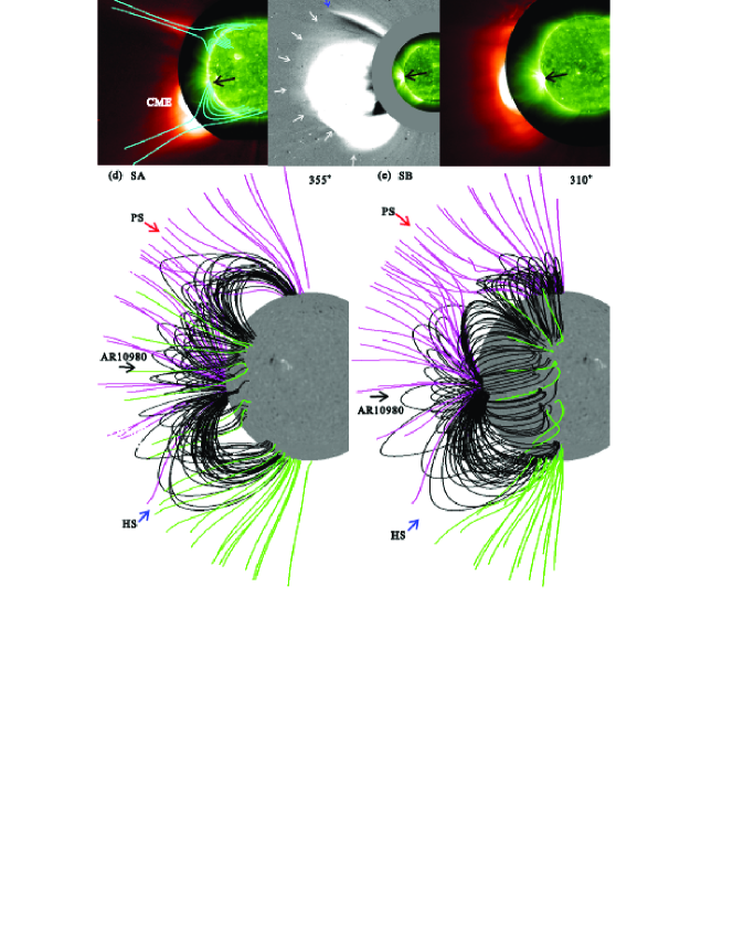
Figure 1: (a-c) EUV and white light observations of the CME from SA, SOHO, and SB on December 31 2007. The angle between SA and SB was 44^∘ at the time of this event. The COR1 ($\sim$ 01:00 UT) and EUVI ($\sim$ 00:55 UT) images from SA and SB and the difference LASCO image together with the EIT data from SOHO are shown. Black arrows denote the eruption source AR10980, white arrows denote the diffuse sheath structure ahead of the bright ejecta, and the blue arrow points to the front of the streamer deflection caused by the shock. (d-e) Coronal magnetic field configurations as given by the PFSS model based on the magnetic field measurements with MDI for the Carrington Rotation 2065. The magnetic configurations have been rotated to the view angles of SA and SB, respectively. The estimated overall magnetic topologies of the PS and HS are plotted with cyan lines in (a).

In Figures 1a-1c we present three sets of EUV and white light observations of the CME from SA, SOHO, and SB. The angle between SA and SB was 44^∘ at the time of this event. The superposed Inner Coronagraph (COR1) at $\sim$ 01:00 UT and Extreme UltraViolet Imager (EUVI) at $\sim$ 00:55 UT images from SA and SB and the difference Large Angle and Spectrometric Coronagraph (LASCO) image together with the Extreme-ultraViolet Imaging Telescope (EIT) data from SOHO are shown. Black arrows denote the eruption source active region (AR)10980, which is located at about E102S08, E58S08, and E81S08 as viewed from SA, SB, and SOHO (http://www.lmsal.com/solarsoft/). So, the CME is seen as a near-limb event by all three spacecraft. This greatly constrains the projection effect on the measurements of the CME dynamics. The CME is first observed by COR1A and COR1B at 00:55 UT and by LASCO C2 at 01:31 UT. The corresponding CME leading edges are located at 1.55, 1.65, and 4.80 R_⊙, respectively. A C8.3 flare is associated with the CME. According to the GOES observation, the X-ray flux starts to increase rapidly at 00:30 UT, and reaches its peak at 00:50 UT.

As clearly seen from the SA and SOHO observations, streamers are present on both sides of the CME source. Figures 1d and 1e present the coronal magnetic field configurations from the potential-field source-surface model (PFSS; Schatten et al., 1969; Schrijver & Derosa 2003) based on the magnetic field measurements with Michelson Doppler Imager (MDI; Scherrer et al., 1995) for the Carrington Rotation 2065. The magnetic configurations have been rotated to the view angles of SA and SB, respectively. Large-scale closed field lines, corresponding to the white light streamers, can be seen on both sides of the active regions. The northern streamer is narrower and weaker than the southern one. This is consistent with the fact that the northern streamer is a pseudo streamer (PS: Wang et al., 2007; Liu et al., 2009b) while the southern streamer is a typical helmet streamer (HS). For a PS, the polarities of the open field enclosing the streamer-like structure are the same, as seen from the PFSS results. In Figure 1a, we delineate the estimated overall magnetic topologies of both streamers with cyan lines.

Several additional features in Figures 1a-1c worth to be noted. First, as seen from the LASCO difference image, there is a diffuse structure ahead of the bright CME front. Such a structure is usually regarded as the signature of shock sheath (Vourlidas et al., 2003). Small white arrows point to different locations of the sheath front. As a result of the asymmetric expansion of the CME, the stand-off distance varies significantly along the front. Second, the PS is deflected significantly as shown from the obvious white-black difference structure, even in the absence of direct contact with the bright ejecta. Streamer deflection without a CME contact has been attributed to the CME-driven shock (e.g., Sheeley et al., 2000). Finally, there is a concave-outward structure at the CME front along the direction of the stalk of the southern streamer, which is usually interpreted as a result of a CME propagating into denser and slower plasma sheet structure (see, e.g., Riley & Crokker, 2004; Odstrcil et al., 2004). This concave-outward structure therefore indicates a very strong interaction of the CME with this streamer. As to be shown below, this observation is consistent with the SA data.

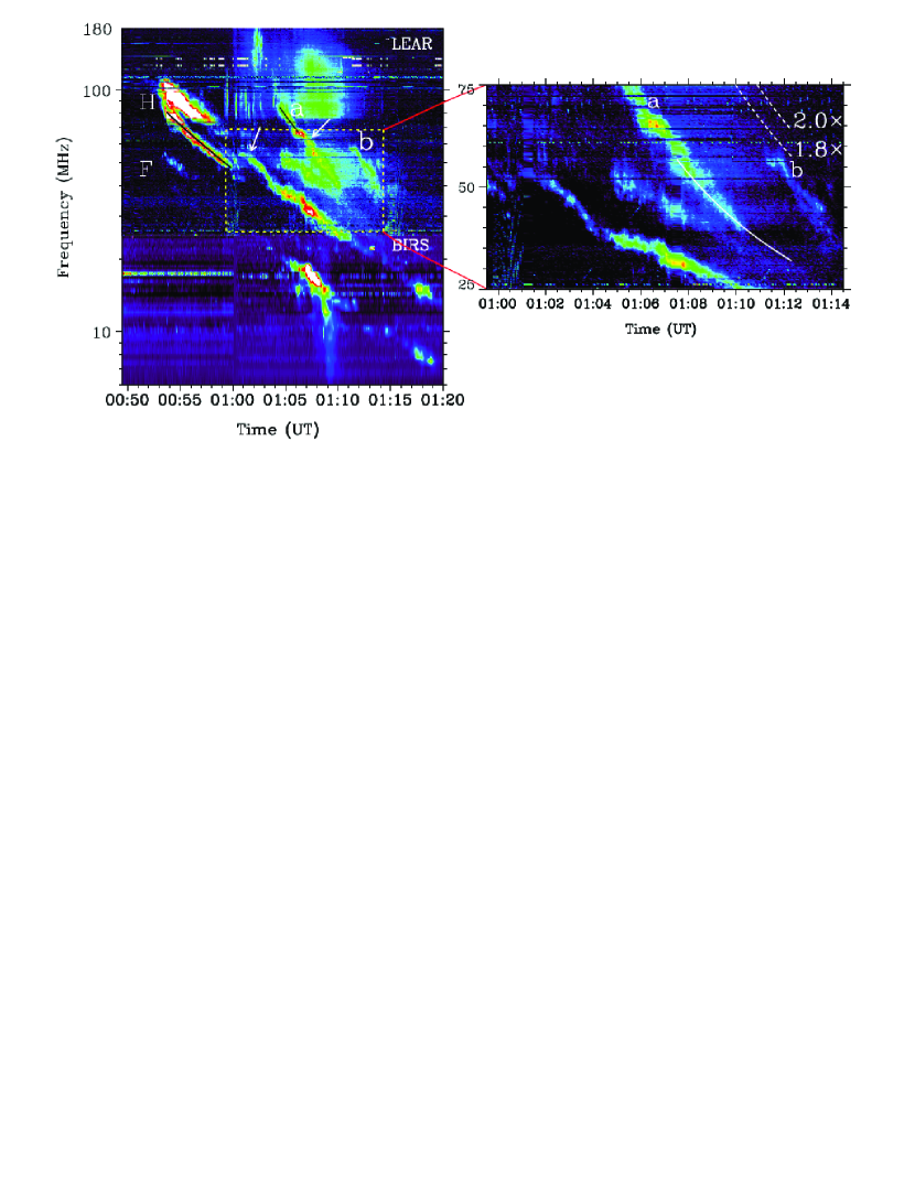
Figure 2: Left: the dynamic spectrum of the associated multiple type II radio burst as recorded by Learmonth and BIRS radio spectrometers. Three type II episodes are observed. The first episode shows fundamental (F) and harmonic (H) branches with clear signatures of band splitting of H branch. The other two episodes are denoted by “a” and “b”. White arrows indicate the spectral bump features on the first two episodes. The black lines are the fitting curves using the 1$\times$ Saito density model and a shock speed of 530 km s^-1 for the first episode and 650 km s^-1 for the second using 0.4$\times$ Saito density model. Right: an enlargement of the spectrum in square region of the left panel with the y-axis in a linear scale. The solid white line is the fitting curve of the post-bump part of “a” using 0.4$\times$ Saito density model and a shock speed of 550 km s^-1. The upper two dashed white lines are given by 1.8 and 2 times larger than this fitting curve.

Now we turn our attention to the dynamic spectrum of the associated radio burst, which was recorded by Learmonth (Kennewell & Steward 2003) and BIRS (Bruny Island Radio Spectrometer; Erickson 1997) and shown in the left panel of Figure 2. An enlargement of the spectrum in the square region is given in the right panel with the y-axis on a linear scale. Several type II episodes are observed. The first episode shows fundamental (F) and harmonic (H) branches with clear signatures of band splitting on the H branch. It starts at $\sim$ 00:53 UT and ends at $\sim$ 01:20 UT lasting for about 30 minutes. The H branch spans from $>$ 100 MHz to 14 MHz.

The other two episodes are denoted by “a” (01:04 UT - 01:10 UT, 85 MHz - 35 MHz) and “b” (01:11 UT - 01:14 UT, 57 MHz - 40 MHz) in Figure 2. These two emissions were regarded as the fundamental and harmonic branches of a type II burst by Gopalswamy et al. (2009) and Cho et al. (2011). However, with a careful examination we conclude that this may not be the case. Note that there are no temporally-overlapping emissions between “a” and “b”. Therefore, to determine their frequency ratio we need to fit the dynamic spectra to allow a direct comparison of their frequencies. The fitting curve to “a” from 01:08 UT - 01:11 UT is drawn by the white solid line in Figure 2, using the 0.4$\times$ Saito density model (Saito et al., 1977). The fitting gives a shock speed of 550 km s^-1 (the reason of employing such a density model is explained in the Appendix). Two white dashed lines with frequencies 1.8 and 2 times larger than the fitted curve are also plotted. It can be seen that the frequency ratio between the emission denoted by “b” and the fitting to “a” is less than $1.8$. This excludes the possibility of “b” being the harmonic counterpart of “a” (Nelson & Melrose, 1985; Mann et al., 1995, 1996). Therefore, we conclude that this multiple type II event consists of three separate episodes of emissions. Since at metric wavelengths the harmonic emission is usually brighter than the fundamental one (e.g., Cairns & Robinson, 1987), we regard “a” to be a harmonic-band emission.

At $\sim$ 01:00 UT the lower band of the H branch of the first episode ($\sim$ 48 MHz) become discontinuous. Shortly after this, the band rises up to a higher frequency of $\sim$ 52 MHz at 01:02 UT, then its frequency decreases rapidly to $\sim 37$ MHz at 01:05 UT. Such a non-monotonic variation of frequencies has been referred to as type II spectral bump by Feng et al. (2012). Another bumping feature, similar in shape, but weaker in amplitude, is present on “a” spanning from $\sim$01:06:10 UT - $\sim$01:07:40 UT around 60 MHz. The two bumps are indicated by white arrows in the figure. Their origin and physical implication are the focus of this study.

Before further discussion, we summarize relevant results from previous studies on this type II event by Liu et al. (2009a), Gopalswamy et al. (2009), and Cho et al. (2011).

Liu et al. (2009a) focused on the driver of the first type II episode. They used the 1.3$\times$ Saito density model (Saito et al., 1977) with a shock speed of 616 km s^-1 to fit the dynamic spectrum and deduce the shock heights. The deduced heights were then compared to the distance measurements of the CME front and the propagating streamer kink induced by the CME shock-streamer interaction. This established the physical connection between the metric and the decametric-hectometric bursts. They concluded that this episode was driven by the CME, rather than by the associated flare. Gopalswamy et al. (2009) measured the height of the CME leading edge at the time of the onset of the first episode and concluded that the type II is emitted at a few tenths of a solar radius above the solar surface. Cho et al. (2011) examined the type II bursts as a multi-band event (e.g., Robinson & Sheridan 1982; Shanmugaraju et al., 2005). They used a Newkirk density model (Newkirk, 1961) to convert the frequencies of the two episodes into shock heights. They found that the obtained two sets of shock heights were consistent with the measured CME-nose heights and the interaction heights of the shock with the northern streamer, respectively. They then concluded that the first episode was excited at the CME shock nose, and the second episode “a” excited at the interaction region of the shock with the northern streamer.

All of the above authors agreed that the type II burst was excited by the CME-driven shock. None of them, however, discussed the bumping features of the spectrum. As noted, these features provide significant amount of information in diagnosing the origin of the type II radio burst. In particular, one may infer the location of the source and physical conditions for the generation of type II radio bursts. We point out that features like these in radio spectra should be carefully examined in relevant CME studies. We note that the back-extrapolation of the second episode “a” maps to the onset of a cluster of type III bursts, which indicates a possible connection to the flare impulsive phase. Therefore, a flare origin of this episode can not be ruled out completely. Nevertheless, we only consider in this study the possibility that the type II emitting shock is driven by the CME.

3 CME-shock profiles and origin of the type II spectral bumps

In this section, we first introduce how we delineate the CME-shock profiles from the EUVI and COR1 data so as to present a clear picture of how the shock evolves and interacts with the streamers. Then, we relate the deduced shock-streamer interactions to the observed type II spectral bumps.

Coronal shock profiles can be determined directly using EUV and white light imaging data. Observational signatures of a coronal shock include diffuse sheath structure ahead of the bright CME ejecta (Vourlidas et al., 2003), deflection and kink of streamer stalks and coronal rays as swept by the CME shock (e.g., Sheeley et al., 2000), and the EUV propagating disturbance revealing the expanding shock front.

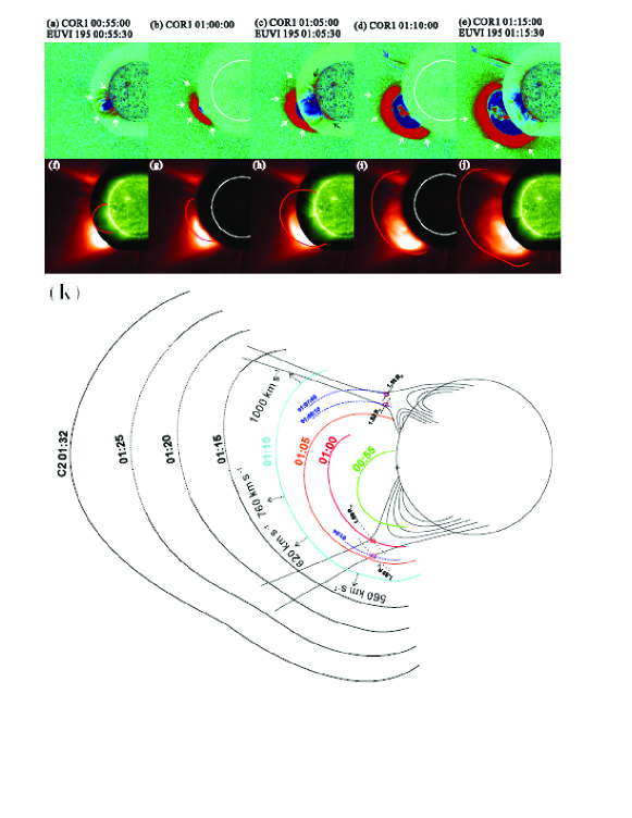
Figure 3: (a-e, f-j) The eruption sequence between 00:55-01:15 UT as observed by COR1 and EUVI of SA. The upper and middle panels present the COR1 running difference images and direct images, respectively, and the EUVI 195 Å difference and direct data are included when available. In panels (a-e), we use arrows of different colors to point out various shock signatures. The resultant continuous shock profiles are plotted in panels (f-j). Corresponding animations can be viewed online. (k) The shock profiles obtained from the above panels. The circle represents the solar limb. The magnetic configurations of the northern and southern streamers are copied from Figure 1a. Also included are the shock profiles as determined from the COR1 running difference images at 01:20 UT and 01:25 UT and the LASCO C2 data at 01:31 UT. The blue dashed shock profiles at 01:04 UT, 01:06:10 UT, and 01:07:40 UT are given by interpolations (or extrapolations) using the obtained average shock speeds along relevant directions of nearby shock profiles, and the two pairs of black dotted arcs are given by r=1.69 R_⊙, 1.83 R_⊙ and r=1.32 R_⊙, 1.38 R_⊙. Small red ellipses represent the intersection points of these arcs with the shock envelopes. See text for more details.

In our event, both the diffuse sheath structure and streamer deflection/kink are observed in the LASCO difference image at 01:32 UT. Since the streamers are best seen by SA (see Figure 1), in Figure 3 we plot the eruption sequence between 00:55 UT-01:15 UT as observed by COR1 and EUVI of SA. The upper and middle panels are the COR1 running difference and direct images, respectively. The EUVI 195 Å difference and direct data are included when available. Corresponding animations can be viewed online.

In the upper panels of Figure 3, we use arrows of different color to point out various shock signatures. The resultant continuous shock profiles are plotted in the lower panels. The solid part of the shock profiles is determined by recognizable shock signatures, and the dotted part represents the profile without a clear shock signature and is derived by assuming a smooth shock propagation.

At 00:55 UT, a bright loop is observed by both EUVI and COR1. This is the first appearance of the CME in the COR1 field of view. None of the above shock signatures are present at this moment mostly because the shock is still rather close to the bright ejecta at this very-early stage of the eruption. Note that the shock is already formed since the corresponding type II burst started earlier at 00:53 UT. We thus take the position of the bright loop structure as the shock front location. Five minutes later (01:00 UT), the loop propagates outward with a fast lateral expansion. A diffuse sheath structure appears at the northeastern quadrant as pointed by the upper arrows. No observable sheath structure is present in the southeastern quadrant partially due to the asymmetric propagation of the CME. The obtained shock profile for 01:00 UT is shown in Figure 3g.

At 01:05 UT, the diffuse sheath structure is well observed ahead of the ejecta in the northeastern quadrant. In addition, from the EUVI 195 Å data we can recognize the EUV fronts associated with the eruption as indicated by the black arrows, which are consistent with the deflection fronts of the EUV rays. We use these features to determine the lower extension of the shock. This allows us to plot a more complete shock envelope than at 01:00 UT. In the southeastern quadrant of the difference image, a weak concave-outward structure along the direction of the stalk of the southern streamer is discernible. The structure is more prominent in the subsequent COR1 data. It was also seen in LASCO, indicating a direct interaction between the CME and the streamer, as mentioned.

At 01:10 UT and 01:15 UT, besides the diffuse sheath structure (see white arrows) a new shock signature appears along the northern streamer as indicated by the blue arrow. The streamer is strongly deflected without a direct contact with the bright ejecta, indicating a shock front propagating along this direction (e.g., Sheeley et al., 2000).

At each time step, we connect the front of the diffuse structure, the front of the streamer deflection, and the concave outward-structure to obtain the full envelope of the CME-driven shock (see Figures 3i and 3j). The obtained shock envelopes are shown all-together in Figure 3k, where the circle represents the solar limb on which the projected eruption source is plotted as the plus sign. The magnetic configurations of the two streamers are copied from Figure 1a. Also included are the shock profiles as determined from the COR1A running difference images at 01:20 UT and 01:25 UT, as well as that given by LASCO C2 at 01:32 UT. Since the angular separation between SOHO and SA is about 22 degrees, the shock profiles seen from SOHO and SA should be similar. This allows us to estimate the shock speeds along different directions. For example, the average speeds in the time range of 00:55 UT - 01:10 UT along four directions pointing from the eruption source (see arrows in Figure 3k) are estimated to 560, 620, 760, and 1000 km s^-1, respectively. These values reveal a very asymmetric propagation of the CME front. The blue dashed shock envelopes at 01:04 UT, 01:06:10 UT, and 01:07:40 UT are given by interpolations between nearby shock profiles or extrapolations using the obtained average shock speeds along relevant directions. Thus, Figure 3k presents a relatively-complete description of the shock propagation from the inner to the outer corona and provides important clues to understanding the origin of type II spectral bumps.

Note that the presence of a spectral bump requires a high density structure along the shock path according to the plasma hypothesis of type II radio bursts (Ginzburg & Zheleznyakov, 1958; Feng et al., 2012). From the coronagraph data alone, both the northern and the southern streamers can be the candidate for the two spectral bumps. From Figures 2 and 3 it can be seen that the first bump ends at 01:04 UT, before the shock contacts the northern PS ($\sim$01:05 UT). This rules out the possibility of the PS accounting for this bump. Further evidence supporting the hypothesis that this spectral bump is caused by the shock transit across the southern streamer can be found by examining the radio-source height. Assuming a 1$\times$Saito density model (see the Appendix), we infer that the radio-source at the onset ($\sim$48 MHz) and the end (37 MHz) of the type II bursts was located at 1.69 R_⊙ and 1.83 R_⊙, respectively. The two heights are presented in Figure 3k with two black dotted arcs. The intersections of these arcs with the shock envelopes are indicated by small red ellipses, which are presumably the source locations of the corresponding type II episode at the onset and the end of the bump.

It can be seen that the two intersections are located at the opposite sides of the pre-disturbed southern streamer. This strongly indicates that the shock transit across this streamer causes the first spectral bump. In addition, from the bump duration ($\tau\sim$ 4 minutes) and the estimated shock speed in this region ($v\sim$ 600 km s^-1, see Figure 3k), one infers the width $D\sim\tau v$ of the dense structure to be 0.2 R_⊙, in agreement with the white light data of the southern streamer. Based on these arguments, we conclude that the first bump is caused by the shock transit across the southern streamer.

The second bump starts at 01:06:10 UT and lasts for $\sim$1.5 minutes. Its beginning is coincident with the first interaction of the shock with the northern PS. As mentioned earlier, the corresponding type II emission is regarded as the harmonic branch. To examine the role of the PS in the formation of the spectral bump, we convert the frequencies at the beginning and end of this bump to shock heights using the 0.4$\times$ Saito model (which is appropriate to describe the density distribution near the PS, see the Appendix). The radio-source heights are found to be 1.32 R_⊙ and 1.38 R_⊙ and we depict these height levels by two dashed arcs in Figure 3k. Their intersections with the shock envelopes at 1:06:10 UT and 1:07:40 UT, marked by small red ellipses, are found to be located at the two sides of the pre-disturbed PS. This is similar to the situation for the first bump. In addition, the product of the bump duration ($\sim$1.5 minutes) and the estimated shock speed ($\sim$1000 km s^-1, see Figure 3k) agrees with the observed streamer width, and the fact that the PS is narrower in width and weaker in brightness (smaller in density) is also consistent with the corresponding spectral bump being weaker in amplitude and shorter in duration. We therefore conclude that the shock transit across the PS causes the second bump.

In summary, by combining the dynamic spectral and imaging data we are able to determine the physical origin of the two spectral bumps. It suggests that the two type II episodes are produced separately at the two flanks of the same CME shock. From the shock envelopes and the estimated coronal magnetic field topologies from the PFSS model, one finds that the shock geometry at the two flanks are more perpendicular or oblique than quasi-parallel.

Last, in Figure 2 we have presented the fitting curves with the 1$\times$ and 0.4$\times$ Saito density models to the pre-bump spectra of the first and the second episodes. From the fittings we deduce the radio source speeds to be 530 km s^-1 for the first episode and 650 km s^-1 for the second episode. Note that in our event the radio source propagates along a highly non-radial direction, so these speeds are representative of the radial components. These values agree with the speed measurements deduced from the white light images as shown in Figure 3k, therefore providing a self-consistency check of the validity of the density model used for the fittings.

4 Discussion on the inferred source size of type II bursts

We point out that observations of spectral bumps of type II radio burst can be employed as a unique method to infer the source size of the type II radio bursts. From the dynamic spectrum we see that the type II emission lane is raised up as a whole within a relatively short interval. This implies that the size of the radio source is smaller than the associated dense streamer structure ($\sim$ 0.1 - 0.3 R_⊙). The short duration of the rising part also suggests that the source is compact in spatial extension. Due to the intermittency of the radio signals at the onset of the first type II bump, we are unable to determine the exact time duration for the spectral elevation. However, one can infer an upper limit of $\sim 1$ minute. Then assuming the shock crosses the streamer with a speed of $\sim$ 600-1000 km s^-1, we deduce that the spatial dimension of the radio source needs to be smaller than 0.05-0.1 R_⊙ at a fundamental frequency level of 20-30 MHz. Comparing to the very broad extension of the shock surface (easily $>$ 1 R_⊙), the type II source can be practically regarded as “point-like”.

Earlier data analyses of radioheliographs revealed that type II sources were restricted to discrete sectors of an arc around the flare center (Wild 1970; Wild & Smerd, 1972), and sometimes of large dimension ($\sim$ 0.5 R_⊙) (Kai & McLean 1968). It is well known that the radio source size obtained by radio-heliographs tends to be larger than the real value due to propagation and scattering of radiation from the source to the observer. Also, earlier radio imaging instruments such as the Culgoora and Clark Lake Radio-heliographs have an angular resolution of several arcminutes at frequencies $<$ 100 MHz, which corresponds to a spatial resolution of a few tenths of a solar radius near the Sun. Therefore these instruments were not able to resolve the type II source as small as that deduced from our study, although the discrete feature of the imaging observations agrees with our result.

The suggestion that the type II source is compact implies that the presence of shocks is only a necessary condition for the generation of type II bursts. Other strict physical conditions must also be satisfied at the shock in order to create a non-thermal distribution of electrons which is unstable to plasma instabilities. For example, the radio-emitting shock front may be quasi-perpendicular, as revealed by our study. Early theoretical studies have proposed that quasi-perpendicular shocks can accelerate electrons by the shock drift acceleration mechanism (Holman & Pesses 1983, Wu 1984). When the shock speed is sufficiently large or $\theta_{Bn}$ (the angle between shock normal and upstream magnetic field) is close to 90 degrees, some electrons can be accelerated to non-thermal energy and excite plasma waves. However it is known that in this process both the fraction and achievable energy of the accelerated particles are limited (e.g., Ball & Melrose 2001). Other effects, such as MHD turbulence, shock ripples and/or magnetic collapsing trap geometries (e.g., Decker, 1990; Zlobec et al., 1993; Magdalenić et al., 2002; Guo & Giacalone, 2010; Schmidt & Carins, 2012; Hillan et al., 2012) may be required to yield more efficient electron acceleration and radio emission. If indeed local structures, such as ripples or magnetic traps, play an important role in accelerating electrons, then it is understandable that the radio-emitting region at the shock front is spatially confined.

In space weather studies, the frequency drift of type II burst is often employed as an important input to predict the shock arrival time at Earth. However, if the type II burst is generated from a special discrete part of the shock flank, as inferred from our study, then the speeds obtained from the curve fitting to the dynamic spectrum may not be accurate. This should be taken into consideration when using type II spectrum as inputs to drive space weather forecastings.

5 Conclusions

In this paper we investigated the physical origin of two bump features on the dynamic spectrum of a multiple type II radio burst, which were associated with a CME event occurred on December 31 2007. Combining radio spectral data and EUV/white light imaging observations, we found that the type II bumps are caused by the source density variation when the CME shock propagates through nearby dense streamers. It is suggested that the two type II episodes are generated separately at the two flanks of the CME-driven shock. It is further inferred that the type II signals are emitted from discrete spatially-confined sources at the CME-shock flank with the source spatial extension smaller than 0.05-0.1 R_⊙ at a fundamental frequency level of 20-30 MHz and the large-scale shock geometry is close to quasi-perpendicular and/or oblique.

Appendix A Appendix: Coronal electron density distribution deduced with the pB inversion method

The coronal electron density ($n_{e}$) distribution can be deduced by inverting the polarization brightness (pB) data recorded by coronagraphs. In Figure 4a, we show the pB data observed by LASCO C2 at 21:05 UT on December 30 2007, $\sim$ 4 hours before the type II radio burst. We assume that the coronal background density distribution does not change significantly during this period. Note that the COR1/2 coronagraphs on board STEREO also record the pB data during this event, however, the subtraction of background emission which is dominated by the scattering of dusts on the objective lens does not allow one to determine $n_{e}$ outside of dense streamer regions (c.f., Frazin et al., 2012). Considering the separation angle between SOHO and STEREO A is relatively small ($\sim$22 degrees) and the similarity between the LASCO image and the COR1A image, we use the LASCO pB data to derive $n_{e}$ for our study.

The standard pB inversion method given in the SolarSoft package is used. Radial profiles of $n_{e}$ along three position angles covering most of the CME expansion region are deduced and plotted in Figure 4b. It can be seen that $n_{e}$ distributes asymmetrically. At the regions close to the southern and northern streamer, $n_{e}$ can be well represented by 1$\times$ and 0.4$\times$ Saito density model (Saito et al., 1977), respectively. Furthermore, $n_{e}$ generally decreases from the southern to the northern streamer, as indicated by latitudinal variation of pB values at two distances (2.5 R_⊙ and 3 R_⊙ see Figure 4c). The projected angular width of the southern (northern) streamer is $\sim$10 (5) degrees.

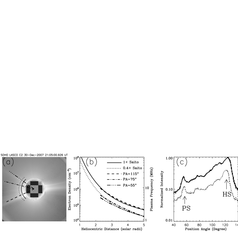
Figure 4: (a) The pB data observed by LASCO C2 at 21:05 UT on December 30 2007; (b) Radial profiles of $n_{e}$ along three position angles as deduced with the standard pB inversion method, the density profiles given by 1$\times$ and 0.4$\times$ Saito density model are depicted by the solid and dotted line, respectively; (c) Latitudinal variations of normalized pB intensity at two distances of 2.5 R_⊙ (solid) and 3.0 R_⊙ (dotted).

References

- Antunes et al. (2009) Antunes, A., Thernisisen, A., & Yahil, A. 2009, Sol. Phys., 259, 199
- (2) Ball, L., & Melrose, D. B. 2001, PASA, 18, 361
- (3) Cairns, I. H., & Robinson, R. D. 1987, Sol. Phys., 111, 365
- Cane & Erickson (2005) Cane, H. V., & Erickson, W. C. 2005, ApJ, 623, 1180
- Cho et al. (2007) Cho, K. S., Lee, J., Moon, Y. J., Dryer, M., Bong, S. C., Kim, Y. H., & Park, Y. D. 2007, A&A, 461, 1121
- Cho et al. (2008) Cho, K. S., Bong, S. C., Kim, Y. H., Moon, Y. J., Dryer, M., Shanmugaraju, A., Lee, J., & Park, Y. D. 2008, A&A, 491, 873
- Cho et al. (2011) Cho, K. S., Bong, S. C., Moon, Y. J., Shanmugaraju, A., Kwon, R. Y., & Park, Y. D. 2011, A&A, 530, 16
- Cliver et al. (1999) Cliver, E. W., Webb, D. F., & Howard, R. A. 1999, Sol. Phys, 187,89
- Cliver et al. (2005) Cliver, E. W., Nitta, N. V., Thompson, B. J., & Zhang, J. 2005, Sol. Phys., 225, 105
- Dai et al. (2012) Dai, Y., Auchere, F., Vial, J. C., Yang, Y. H., & Zong, W. G. 2010, ApJ, 708, 913
- Decker (1990) Decker, R. B. 1990, JGR, 95, 11993
- de Koning et al. (2009) de Koning, C. A., Pizzo, V. J., & Biesecker, D. A. 2009, Sol. Phys., 256, 167
- Dulk (1985) Dulk, G. A. 1985, ARA&A, 23, 169
- Erickson (1997) Erickson, W. C. 1997, Publication Astronomical Society of Austraila, 14, 3, 278-282
- Fent et al. (2012) Feng, S. W., Chen, Y., Kong, X. L., Li, G., Song, H. Q., Feng, X. S., & Liu, Y., 2012, ApJ, 753, 21
- Frazin et al. (2012) Frazin, R. A., Vasquez, A. M., & Thompson, W. T., et al. 2012, Sol. Phys., 280, 273
- Ginzburg & Zhelezniakov (1958) Ginzburg, V. L., & Zhelezniakov, V. V. 1958, SvA, 2, 653
- Gopalswamy et al. (1998) Gopalswamy, N., Kaiser, M. L., & Lepping, R. P., et al. 1998, J. Geophys. Res., 103, 307
- Gopalswamy et al. (2009) Gopalswamy, N., Thompson, W. T., Davila, J. M., Kaiser, M. L., Yashiro, S., Makela, P., Michalek, G., Bougeret, J. L., & Howard, R. A. 2009, Sol. Phys., 259,227
- Gosling (1993) Gosling, J. T. 1993, J. Geophys. Res., 98, 18937
- Guo & Giacalone (2010) Guo, F., & Giacalone, J. 2010, ApJ, 715, 406
- Hillan et al. (2012) Hillan, D. S., Cairns, I. H., & Robinson, P. A. 2012, J. Geophys. Res., 117, A06105
- Holman & Pesses (1983) Holman, G. D., & Pesses, M. E. 1983, ApJ, 267, 837
- Kai & McLean (1968) Kai, K. & McLean, D. L. 1968, PASAu, 1, 141
- Kaiser et al. (2008) Kaiser, M. L., Kucera, T. A., & Davila, J. M., et al. 2008, Space Sci. Rev. 136, 5
- Kennewell & Steward, (2003) Kennewell, J. & Steward, G. 2003, Solar Radio Spectrograph [SRS] Data Viewer [Srsdisplay] (Sydney: IPS Radio and Space Serv.), ftp://ftp.ips.gov.au/wdc-data/spec/doc/Other%20Document/Srsdispl.doc
- Kong et al. (2012) Kong, X. L., Chen, Y., Feng, S. W., Song, H. Q., Li, G., Guo, F., & Jiao, F. R. 2012, ApJ, 750, 158,
- Knock & Cairns (2005) Knock, S. A., & Cairns, I. H. 2005, J. Geophys. Res., 110, A01101
- Lin et al. (2010) Lin C. H., Gallagher, P. T., & Raftery, C. L. 2010, A&A, 516, A44
- (30) Liu, Y., Luhmann, J. G., Bale, S. D., & Lin, R. P. 2009a, ApJ, 691, L151
- (31) Liu, Y., Luhmann, J. G., Lin, R. P., Bale, S. D., Vourlidas, A., & Petric, G. J. D. 2009b, ApJ, 698, 51
- magdalenić (2002) Magdalenić, J., Vršnak, B., & Aurass, H. 2002, Proc. 10th European Solar Physics Meeting, Solar Variability: From Core to Outer Frontiers, ed. A. Wilson (Noordwijk: ESA Publications Division), 335, ESA SP-506
- Magdalenić et al. (2008) Magdalenić, J., Vršnak, B., Pohjolainen, S., Temmer, M., Aurass, H., & Lehtinen, N. J. 2008, Sol. Phys., 253, 305
- Mancuso & Raymond (2004) Mancuso, S., & Raymond, J. C. 2004, A&A, 413, 363
- Mann et al. (1995) Mann, G., Classen, T., & Aurass, H. 1995, A&A, 295, 775
- Mann et al. (1996) Mann, G., Klassen, A., Classen, H. T., Aurass, H., Scholz, D., MacDowall, R. J., & Stone, R. G. 1996, A&ASS, 119, 489
- Moran et al. (2010) Moran, T. G., Davila, J. M., & Thompson, W. T., 2010, ApJ, 712, 453
- Nelson & Melrose (1985) Nelson, G. S., Melrose, D. B. 1985, in: McLean, D. J., Labrum N. R.(eds.) Solar Radiophysics. Cambridge Univ. Press, Cambridge, UK, p. 333
- Newkirk (1961) Newkirk, G. Jr. 1961, ApJ, 133, 983
- (40) Odstrcil, D., & Pizzo, V, J., 2009, Sol. Phys., 259, 309
- Odstrcil et al. (2004) Odstrcil, D., Riley, P., & Zhao, X. P. 2004, JGR, 109, 02116
- Pick & Vilmer (2008) Pick, M., & Vilmer, N. 2008, A&ARv, 16, 1
- (43) Pohjolainen, S., Hori, K., & Sakurai, T. 2008a, Sol. Phys., 253, 291
- (44) Pohjolainen, S., Pomoell, J., & Vainio, R. 2008b, A&A, 490, 357
- Reiner et al. (2003) Reiner, M. J., Vourlidas, A., & Cyr, O. C. St. et al. 2003, ApJ, 590, 533
- Rigozo et al. (2011) Rigozo, N. R., Lago, A. D., & Nordeman, D. J. R. 2011, ApJ, 738, 107
- Riley & Corooker (2004) Riley, P., & Crooker, N. U. 2004, ApJ, 600, 1035
- Robinson & Sheridan (1982) Robinson, R. D., & Sheridan, K. V. 1982, PASA, 4, 392
- Saito et al. (1977) Saito, K., Poland, A. I., & Munro, R. H. 1977, Sol. Phys., 55, 121
- Schatten et al. (1969) Schatten, K. H., Wilcox, J.M., & Ness, N.F. 1969, Sol. Phys., 6, 442.
- Scherrer et al. (1995) Scherrer, P. H., Bogart, R. S., & Bush, R. I. et al. 1995, Sol. Phys., 162, 129
- Schmidt & Cairns (2012) Schmidt, J. M., & Cairns, I. H. 2012, J. Geophys. Res., 117, A04106
- Schrijver & DeRosa (2003) Schrijver, C.J., & De Rosa, M.L. 2003, Sol. Phys., 212, 165.
- Shanmugaraju et al. (2005) Shanmugaraju, A., Moon, Y. J., Cho, K. S., Kim, Y. H., Dryer, M., & Umapathy, S. 2005, Sol. Phys., 232, 87
- Sheeley et al. (2000) Sheeley, N. R., Hakala, W. N., & Wang, Y. M. 2000, J. Geophys. Res. 105, 5081
- Shen et al. (2013) Shen, C. L., Liao, C. J., Wang, Y. M., Ye, P. Z., & Wang, S. 2013, Sol. Phys., 282, 543
- Vourlidas et al. (2003) Vourlidas, A., Wu, S. T., Wang, A. H., Subramanian, P., & Howard, R. A. 2003, ApJ, 598, 1392
- Vršnak & Cliver (2008) Vršnak, B., & Cliver, E. W. 2008, Sol. Phys., 253, 215
- Wang et al. (2007) Wang, Y. M., Sheeley, N. R. Jr., & Rich, N. B. 2007, ApJ, 658, 1340
- (60) Wanger, W. J., & MacQueen, R. M. 1983, A&A, 120, 136
- Wild (1950) Wild, J. P. 1950, Aust. J. Sci. Res. A: Phys. Sci., 3, 399
- Wild (1970) Wild, J. P. 1970, PASAu, 1, 365
- Wild & Smerd (1972) Wild, J. P., & Smerd, S. F. 1972, ARA&A, 10, 159
- Wu (1984) Wu, C. S. 1984, J. Geophys. Res., 89(A10), 8857
- Zlobec (1993) Zlobec, P., Messerotti, M., Karlicky, M., & Urbarz, H. 1993, Sol. Phys., 144, 373