Screening properties of Gaussian electrolyte models,
with application to dissipative particle dynamics

Abstract

We investigate the screening properties of Gaussian charge models of electrolyte solutions by analysing the asymptotic behaviour of the pair distribution functions. We use a combination of Monte-Carlo simulations with the hyper-netted chain integral equation closure, and the random phase approximation, to establish the conditions under which a screening length is well defined and the extent to which it matches the expected Debye length. For practical applications, for example in dissipative particle dynamics, we are able to summarise our results in succinct rules-of-thumb which can be used for mesoscale modeling of electrolyte solutions. We thereby establish a solid foundation for future work, such as the systematic incorporation of specific ion effects.

I Introduction

Dissipative particle dynamics (DPD) has seen widespread uptake in modelling soft condensed matter Frenkel and Smit (2002); Noro et al. (2003). The attractions are obvious: by coarse graining over the atomistic degrees of freedom one can access the relevant length and time scales with only modest computing requirements. Polymer phase behaviour Groot and Warren (1997); Groot and Madden (1998), polymer dynamics Spenley (2000), polymer rheology Sultan et al. (2010), surfactant mesophase formation kinetics Prinsen et al. (2002), the properties of amphiphilic bilayers Groot and Rabone (2001); Shillcock and Lipowsky (2002), and the properties of colloidal suspensions Boek et al. (1997) have all been investigated by the method.

Charged systems such as anionic and cationic surfactants, water-soluble polyelectrolytes, charge-stabilised colloidal suspensions, and mixtures of these Groot (2003), form a large subclass of widespread practical importance. In these systems there is often the requirement to model the supporting electrolyte. This can be done implicitly, for example with the Poisson-Boltzmann equation, or explictly by incorporating ions as charged particles in the simulation. In the latter case, particularly for DPD where soft interactions are the norm, it is natural to smear the point charges into charge clouds. The divergence of the long-range Coulomb law as $r\to 0$ (where $r$ is the center-center separation) is replaced by a smooth cutoff, thus ensuring thermodynamic stability according to a theorem by Fisher and Ruelle Fisher and Ruelle (1966).

The precise form of the charge smearing is often tuned to the choice of numerical algorithm and a consensus on the best approach has yet to emerge. Groot introduced a grid-based method with linear charge smearing Groot (2003). Later González-Melchor et al. examined an Ewald-based method with exponential charge smearing González-Melchor et al. (2006). Here we study a related Ewald method with Gaussian charge smearing. This choice can be used to simplify the Ewald algorithm, and connects with recent work on the so-called ultrasoft restricted primitive model (URPM) Coslovich et al. (2011a, b); Nikoubashman et al. (2012). In principle the differences between smearing methods can be subsumed into short-range part of the interparticle potential, though the details are the subject of ongoing investigations.

To study the screening properties of our Gaussian electrolyte model, we use a combination of Monte-Carlo (MC) simulations, the hyper-netted chain (HNC) integral equation closure, and the random phase approximation (RPA), to analyse the asymptotic behaviour of the pair distribution functions. The programme is as follows. In the next two sections we define the mesoscale electrolyte model and the tools used to analyse it. We then present results demonstrating that, for typical applications, HNC can be relied upon to deliver accurate results (it is no exaggeration to say that HNC is up to ten million times faster than MC). We then use HNC to explore the screening properties of the model, establishing the conditions under which a screening length is well defined (i. e. on the low density side of a Kirkwood line in the phase diagram) and the extent to which the screening length matches the expected Debye length. We further establish the domain of applicability of the much simpler RPA, which gives relatively simple expressions for the Kirkwood line and the screening length. We emphasise that our approach could easily be applied to other smeared charge electrolyte models. Mindful of this, and the utility of a fast, accurate, multicomponent HNC solver in general, we have released our FORTRAN 90 HNC code as fully documented open source software OZn .

II Model

We now describe the Gaussian charge model for electrolyte solutions. The potential energy is given by a sum of pairwise terms, split into short range and long range (electrostatic) contributions,

$$U=\sum_{i>j}U_{ij},\quad U_{ij}=U^{\mathrm{S}}_{ij}+U^{\mathrm{L}}_{ij}\,.$$ (1)

The short range piece is given by

$$\beta U^{\mathrm{S}}_{ij}=\left\{\begin{array}[]{ll}\frac{1}{2}A_{ij}(1-r_{ij}/r_{c})^{2}&(r_{ij}<r_{c})\\[3.0pt] 0&(r_{ij}\geq r_{c})\end{array}\right.$$ (2)

and the long range piece is given by

$$\beta U^{\mathrm{L}}_{ij}=\frac{l_{\mathrm{B}}z_{i}z_{j}}{r_{ij}}\operatorname{erf}\Bigl{(}\frac{r_{ij}}{2\sigma}\Bigr{)}\,.$$ (3)

In these $\beta=1/k_{\mathrm{B}}T$ is the inverse of the temperature $T$ measured in units of Boltzmann’s constant $k_{\mathrm{B}}$, $r_{ij}$ is the centre-centre separation between particles $i$ and $j$, $A_{ij}$ is a dimensionless short range repulsion amplitude which depends on the particle types, $l_{\mathrm{B}}$ is the Bjerrum length which plays the role of an electrostatic coupling constant, $z_{i}$ and $z_{j}$ are the valencies measured in units of an elementary charge, and $r_{c}$ and $\sigma$ are length scales which measure, respectively, the range of short range repulsion and the size of the Gaussian charge cloud. The short range part of the potential corresponds to the standard DPD interaction law Groot and Warren (1997). The long range part corresponds to the interaction between Gaussian smeared charges with a radial charge distribution $(2\pi\sigma^{2})^{-3/2}\exp({-r^{2}/2\sigma^{2}})$. The function $\operatorname{erf}(r/2\sigma)\to r/(\sigma\sqrt{\pi})$ as $r\to 0$, thus ensuring the Coulombic divergence is replaced by a smooth cutoff.

We will consider up to three species of particles, corresponding to positively and negatively charged ions of valencies $z_{+}$ and $z_{-}$ at densities $\rho_{+}$ and $\rho_{-}$, and a third neutral solvent species at a density $\rho_{0}$. The total ion density will be denoted by $\rho_{z}=\rho_{+}+\rho_{-}$. The total overall density will be denoted by $\rho=\rho_{0}+\rho_{z}$. In the case where there is no solvent, $\rho_{0}=0$ and $\rho=\rho_{z}$. We adopt the convention that the valency includes the sign as well as the magnitude. Overall charge neutrality then requires $z_{+}\rho_{+}+z_{-}\rho_{-}=0$. We do not necessarily suppose the valencies are of the same magnitude. We shall label species by Greek indices, $\alpha,\beta=(0,+,-)$. The system volume is $V$ and thermal averages will be denoted by $\langle\cdot\rangle$.

We first consider a special case. The aforementioned URPM is an unsolvated equimolar mixture of Gaussian charge clouds, corresponding to the choice $A_{ij}=0$, $\rho_{0}=0$, and $|z_{\pm}|=1$. The URPM is governed by a dimensionless density, $\rho_{z}\sigma^{3}$, and a dimensionless coupling constant, $l_{\mathrm{B}}/\sigma$, which plays the role of an inverse temperature. The model exhibits marked clustering for $l_{\mathrm{B}}/\sigma\gtrsim 30$, and a condensation transition for $l_{\mathrm{B}}/\sigma\gtrsim 100$, for densities in the range $\rho_{z}\sigma^{3}\approx 0.01$–0.1 (these estimates are translated from the results shown in Fig. 5 in Ref. Coslovich et al., 2011a). The physics behind the phase transition remains somewhat unclear Nikoubashman et al. (2012); Warren and Masters (2013), but the phenomenology can be viewed as a reflection of stability issue for point charges mentioned in the introduction. It quantifies the onset of the ‘danger zone’ as the point charge limit is approached. To avoid these artefacts the implication is that we should attempt to keep $l_{\mathrm{B}}/\sigma\lesssim 30$. However for practical applications there is already a strong incentive to make $\sigma$ as large as possible, to reduce the cost of computing the electrostatic interactions. Usually this is enough to ensure that low temperature URPM artefacts are avoided.

In the general case the properties of the model are governed by three length scales, $r_{c}$, $\sigma$ and $l_{\mathrm{B}}$, the repulsion amplitude matrix $A_{ij}$, the choice of valencies $z_{\pm}$, and the densities $\rho_{z}$ and $\rho$. The parameter space is thus potentially very large. Our strategy to reduce the complexity is to consider the mapping to the underlying atomistic system. This requires us to distinguish between physical units in which the length scales and densities are expressed in SI units; and simulation units in which length scales and densities are expressed in units of $r_{c}$ or $\sigma$.

In standard DPD the choice $\rho r_{c}^{3}=3$ is usually made Groot and Warren (1997), and we will adopt the same here. In addition one usually introduces the notion of a ‘mapping number’ $N_{m}$, giving the number of solvent molecules represented by one DPD solvent particle. Given this, the value of $r_{c}$ in physical units is determined by the identity $\rho N_{m}V_{m}/N_{A}\equiv 1$, where $V_{m}$ is the solvent molar volume and $N_{A}$ is Avogadro’s number González-Melchor et al. (2006). If water is the solvent ($V_{m}=18\times 10^{-6}\,\mathrm{mol}\,\mathrm{m}^{-3}$), and with the conventional choice $N_{m}=3$, one has in physical units $r_{c}=0.645\,\mathrm{nm}$.

Next consider the Bjerrum length. In physical units this is $l_{\mathrm{B}}=e^{2}/(4\pi\epsilon_{r}\epsilon_{0}k_{\mathrm{B}}T)$ where $e$ is the elementary charge, $\epsilon_{r}$ is the relative permittivity of the solvent, and $\epsilon_{0}$ is the permittivity of free space. For water at room temperature $l_{\mathrm{B}}\approx 0.7\,\mathrm{nm}\approx 1.09\,r_{c}$. Since a $z$:$z$ electrolyte is equivalent to a 1:1 electrolyte with $l_{\mathrm{B}}$ increased by a factor $z^{2}$, there is considerable interest in exploring higher values of $l_{\mathrm{B}}$. In the present work we shall explore up to $l_{\mathrm{B}}=10\,r_{c}$ (${}\approx 7\,\mathrm{nm}$ in physical units), which covers many cases of interest.

For an electrolyte at a molar concentration $c_{s}$, the microscopic ion density is $10^{3}c_{s}N_{A}$. This is readily converted to a simulation density by multiplying by $r_{c}^{3}$. For example a $0.1\,\mathrm{M}$ 1:1 electrolyte solution would be represented by $\rho_{z}r_{c}^{3}=0.032$ (note that $\rho_{z}$ counts both species of ion). To cover the typical range of electrolyte concentrations we therefore consider $\rho_{z}r_{c}^{3}$ in the range $10^{-3}$–1.

The above considerations do not yet impinge on the choice of $\sigma$. This is a central theme of the present study and will be discussed extensively below.

Finally we discuss the repulsion amplitude matrix. In the present study we will only consider a constant repulsion amplitude matrix $A_{ij}=A$, leaving the extension to unequal repulsion amplitudes for future work. We use either $A=25$ motivated by standard DPD Groot and Warren (1997), or $A=0$ corresponding to the situation in the absence of short range repulsions. In the latter case, of course, it does not make sense to include the neutral solvent species since it would just form an ideal gas in the background. It has been suggested that $A$ should be chosen to match the solvent compressibility Groot (2003). However this introduces the danger if $A$ is too large one will encounter an order-disorder transition driven by the short range repulsions. A less rigorous criterion is to demand only that the solvent be relatively incompressible, so that $\partial(\beta p)/\partial\rho\gg 1$ where $p$ is the pressure. This is satisfied by $A=25$, for which the solvent is clearly still a liquid with only moderate structure. Moreover much work has been done based on this value, which we will therefore continue to use.

To summarise, in the remainder of this work we shall consider mainly two classes of models: either the pure URPM comprising unsolvated Gaussian charges, or the ‘solvated’ case containing in addition a neutral species and short range repulsions between all particles. (It is possible to consider an intermediate case where short range repulsions are added to the URPM, however this does not generate any new insights.) As already mentioned the URPM is characterised by the dimensionless density $\rho_{z}\sigma^{3}$ (with $|z_{\pm}|=1$ implying $\rho_{\pm}=\rho_{z}/2$) and coupling strength $l_{\mathrm{B}}/\sigma$. The length scale $r_{c}$ plays no role, except, perhaps, as a ‘fiducial’ length. On the other hand the solvated case (with the ‘standard’ choice $\rho r_{c}^{3}=3$ and $A=25$) is characterised by the dimensionless densities $\rho_{\pm}r_{c}^{3}$, and dimensionless ratios $l_{\mathrm{B}}/r_{c}$ and $\sigma/r_{c}$, where all except $\sigma/r_{c}$ are fixed by the mapping to the underlying physical system.

From a practical point of view $\sigma\neq r_{c}$ is commonplace, and it shall be important to pay attention to the units of length when mapping between the solvated case and the pure URPM. In the text we shall endeavour to be always explicit about this, and where the figure annotations use implicit units we shall always state the choice of units in the caption. A symmetric $z$:$z$ electrolyte in the solvated case can be mapped to the URPM with a renormalised $l_{\mathrm{B}}\to z^{2}l_{\mathrm{B}}$. An asymmetric electrolyte cannot be mapped onto the URPM but we shall discuss this case only rather briefly. It is worth bearing in mind that it is quite straightforward to apply the tools developed here to all these cases.

III Tools

III.1 Pair distribution functions and screening

Given the model is governed solely by pair interactions, the thermodynamic properties are completely determined by the pair distribution functions $g_{\alpha\beta}(r)$. In addition the screening properties are also determined by the asymptotic behaviour of these functions. Specifically, the screening length $\lambda$ features in the asymptotic behaviour of the total correlation functions,

$$h_{\alpha\beta}(r)\equiv g_{\alpha\beta}(r)-1\sim\frac{e^{-r/\lambda}}{r}\quad(r\to\infty)$$ (4)

provided the asymptotic decay is purely exponential. The decay length defined in this way is unique to each state point and does not depend on the identity of the species of charged particles under consideration.

As the density decreases the screening length approaches the Debye-Hückel limiting law behaviour, $\lambda\to\lambda_{\mathrm{D}}$, where the Debye length is

$$\lambda_{\mathrm{D}}=({\textstyle 4\pi l_{\mathrm{B}}\sum_{\alpha}\!z_{\alpha}^{2}\rho_{\alpha}})^{-1/2}\,.$$ (5)

Conversely, as the density increases the screening length gets smaller but there comes a point where the asymptotic decay of the total correlation functions ceases to be purely exponential and instead becomes damped oscillatory. This transition defines a line in the phase diagram known in charged systems as the Kirkwood line Kirkwood (1936), or more generally a Fisher-Widom line Fisher and Widom (1969).

For applications, one would hope that the actual screening length will hew as closely as possible to the expected Debye length (at least, as long as the latter is well defined). The extent to which this can be made so is the central theme of the present work. For example, a 1:1 electrolyte at $0.1\,\mathrm{M}$ concentration has a Debye length $\lambda_{\mathrm{D}}\approx 0.96\,\mathrm{nm}\approx 1.5\,r_{c}$. If we simulate this in the present model with the choice $\sigma=r_{c}$, the asymptotic decay of the total correlation functions would be oscillatory and we would not even be on the right side of the Kirkwood line. On the other hand if we use $\sigma=r_{c}/2$ the asymptotic decay would be purely exponential with $\lambda/\lambda_{\mathrm{D}}=0.94$, thus the actual screening length would be only 6% different from the Debye length. This example will be worked through in more detail below.

III.2 Integral equation theory

Given that the underlying electrolyte model is a fluid mixture, it is natural to think of using multicomponent integral equation theory to calculate the structural and thermodynamic properties Hansen and McDonald (2006); Ng (1974); Kelley and Montgomery Pettitt (2004); Vrbka et al. (2009). Further, since the interactions are soft, one expects that the hyper-netted chain (HNC) integral equation closure should work well. We find this is indeed the case. We also find that for parameters typical of 1:1 electrolytes, the random phase approximation (RPA) also works well.

The starting point is the multicomponent Ornstein-Zernike (OZ) relation which defines the direct correlation functions $c_{\alpha\beta}(r)$. In reciprocal space the OZ relation is

$${\tilde{h}}_{\alpha\beta}={\tilde{c}}_{\alpha\beta}+{\textstyle\sum_{\gamma}}\,\rho_{\gamma}\,{\tilde{c}}_{\alpha\gamma}\,{\tilde{h}}_{\gamma\beta}$$ (6)

where the spatial Fourier transform of a function $x(r)$ is defined by $\tilde{x}(k)=\int\!d^{3}{\mathbf{r}}\,e^{-i{\mathbf{k}}\cdot{\mathbf{r}}}\,x(r)$. The HNC closure is defined in real space, and is

$$h_{\alpha\beta}=\exp(-\beta U_{\alpha\beta}+h_{\alpha\beta}-c_{\alpha\beta})-1$$ (7)

where $U_{\alpha\beta}$ is the pair potential between particles of species $\alpha$ and $\beta$. The solution of these coupled equations is numerically quite demanding and in the present case we exploit the accelerated convergence schemes originally proposed by Ng Ng (1974); Kelley and Montgomery Pettitt (2004); Vrbka et al. (2009). We typically solve the distribution functions on a grid of size 4096 points at a grid spacing $0.01\,r_{c}$, so that the functions are calculated out to $r\approx 40\,r_{c}$ where all trace of structure has typically vanished below the numerical precision of the calculation. We find, however, that the schemes fail to converge for $l_{\mathrm{B}}/\sigma\gtrsim 10$. This loss of solution has also been observed by Coslovich, Hansen and Kahl Coslovich et al. (2011b), and may be indicative of a mathematical property of the HNC rather than a numerical problem.

Numerically much less demanding is the RPA closure, which is given by

$$c_{\alpha\beta}=-\beta U_{\alpha\beta}\,.$$ (8)

Because there are no hard cores, the RPA is the same as the mean spherical approximation (MSA). Unlike the HNC, the RPA can be solved for all values of $l_{\mathrm{B}}/\sigma$ although it may yield unphysical results (for example $h_{\alpha\beta}<-1$).

The pressure $p$ and the internal energy density $\langle U\rangle/V$, can be solved from the pair functions Hansen and McDonald (2006); Vrbka et al. (2009). The pressure can be found either by the virial or compressibility routes. These do not give exactly the same result because the HNC closure breaks thermodynamic consistency. In practice, for the present applications, we have found the two routes differ by typically at most a few percent. Specific results for the RPA thermodynamics can be found in Refs. Nikoubashman et al., 2012 and Warren and Masters, 2013.

III.3 RPA solution of the URPM

Coslovich, Hansen and Kahl solve the RPA for the URPM Coslovich et al. (2011b), and we have recently revisited the problem in terms of the low temperature phase behaviour Warren and Masters (2013). The relevant properties of the RPA solution are described here. URPM symmetry implies that in the RPA the correlation functions are given by $h_{\pm\pm}(r)=\pm h(r)$. Inserting this into the OZ equations, with the RPA closure, reveals

$$\tilde{h}(k)=\frac{-4\pi l_{\mathrm{B}}\exp({-\sigma^{2}k^{2}})}{k^{2}+k_{\mathrm{D}}^{2}\exp({-\sigma^{2}k^{2}})}$$ (9)

where $k_{\mathrm{D}}^{2}=4\pi l_{\mathrm{B}}\rho_{z}$ is the square of the Debye wavevector (i. e. $k_{\mathrm{D}}=1/\lambda_{\mathrm{D}}$).

The real space total correlation functions can (in principle) be obtained by expressing the Fourier back-transform of Eq. (9) as a contour integral in the complex $k$-plane. The behaviour of the correlation functions is therefore determined by the poles of $\tilde{h}(k)$ in the upper half plane. As a particular consequence, the asymptotic behaviour of $h(r)$ as $r\to\infty$ is determined by the position(s) of the pole(s) closest to the real axis Hopkins et al. (2006); Nikoubashman et al. (2012). There are two cases. If the nearest pole to the real axis is purely imaginary, the asymptotic behaviour of $h(r)$ is purely exponential, with a decay length set by the distance of the pole from the real axis. Alternatively if the nearest poles to the real axis are complex, the asymptotic behaviour is damped oscillatory. Clearly, then, the Kirkwood line is determined by the crossover between these two scenarios, typically when a purely imaginary pole nearest to the real axis collides with the next-nearest pole, to form a complex pair which subsequently move off the imaginary axis.

In the present case, writing $q=\sigma k$ and $q_{\mathrm{D}}=\sigma k_{\mathrm{D}}$, the poles of $\tilde{h}(q)$ are determined by the solutions of

$$q^{2}\exp(q^{2})=-q_{\mathrm{D}}^{2}\equiv-4\pi l_{\mathrm{B}}\rho_{z}\sigma^{2}\,.$$ (10)

These solutions can be expressed in terms of the Lambert $W$ function which solves $We^{W}=z$. For the asymptotic behaviour of $h(r)$ the most relevant solution is given by $q^{2}=W_{0}(-q_{\mathrm{D}}^{2})$ where $W_{0}$ is the principal branch of the Lambert $W$ function Corless et al. (1996); Wno . If $q_{\mathrm{D}}^{2}\leq 1/e$, $W_{0}(-q_{\mathrm{D}}^{2})$ is negative real and the corresponding poles of Eq. (9) (in the complex $q$-plane) are at $q=\pm i|W_{0}(-q_{\mathrm{D}}^{2})|^{1/2}$. The corresponding decay length is given by

$$\lambda_{\mathrm{RPA}}=\sigma\times|W_{0}(-4\pi l_{\mathrm{B}}\rho_{z}\sigma^{2})|^{-1/2}\,.$$ (11)

Note that $\lambda_{\mathrm{RPA}}\to\lambda_{\mathrm{D}}$ (from below) as $\rho_{z}\to 0$. If $q_{\mathrm{D}}^{2}>1/e$, $W_{0}(-q_{\mathrm{D}}^{2})$ is complex and the asymptotic decay of $h(r)$ is damped oscillatory. We therefore identify $q_{\mathrm{D}}^{2}=1/e$ as the Kirkwood line Nikoubashman et al. (2012). Equivalently, Eq. (11) requires

$$4\pi el_{\mathrm{B}}\rho_{z}\sigma^{2}\leq 1\,,$$ (12)

with equality determining the location of the RPA Kirkwood line. For general applications the charge density in Eqs. (11) and (12) should be taken to be the ionic strength, defined by $\rho_{z}=\sum_{\alpha}\!z_{\alpha}^{2}\,\rho_{\alpha}$. The RPA can of course be solved for the solvated URPM case. We leave discussion of this to a separate publication.

III.4 Monte-Carlo methods

We benchmark HNC against MC simulations. We use an $NVT$ ensemble with standard single particle trial displacements in the usual Metropolis scheme Frenkel and Smit (2002). We calculate the energy of a configuration from $U=U^{\mathrm{S}}+U^{\mathrm{L}}$, where $U^{\mathrm{S}}=\sum_{i>j}U^{\mathrm{S}}_{ij}$ from Eq. (2), and $U^{\mathrm{L}}=\sum_{i>j}U^{\mathrm{L}}_{ij}$ from Eq. (3). The latter is re-expressed as an Ewald sum,

$$\beta U^{\mathrm{L}}=\frac{2\pi l_{\mathrm{B}}}{V}\!\sum_{k\leq k_{c}}\!\!A_{k}\,|Q_{\mathbf{k}}|^{2}-\frac{1}{2\sigma\sqrt{\pi}}\sum_{i}z_{i}^{2}$$ (13)

where $A_{k}=k^{-2}\exp({-\sigma^{2}k^{2}})$, and $Q_{\mathbf{k}}=\sum_{i}z_{i}e^{-i{\mathbf{k}}\cdot{\mathbf{r}}_{i}}$ is the reciprocal space charge density. This is just the standard Ewald result omitting the real space contribution Allen and Tildesley (1987); Frenkel and Smit (2002). The last term is a self energy correction; this can of course be omitted from the MC acceptance criterion, but it is essential to retain this correction when making comparisons with integral equation theory.

The first term in Eq. (13) is a sum over a discrete set of wavevectors, commensurate with the simulation box dimensions, such that $k=|{\mathbf{k}}|\leq k_{c}$ where the cut-off is chosen so that $\exp({-\sigma^{2}k_{c}^{2}})$ is sufficiently small. For the simulations reported below we use $\sigma k_{c}=4$. There are about $4\pi k_{c}^{3}/3\times(2\pi)^{3}/V$ discrete wavevectors in the sum (the second factor is the density of wavevectors in reciprocal space). This means that the computational cost of evaluating the sum varies as $1/\sigma^{3}$. As a practical consideration, this is a strong motivation for making $\sigma$ as large as possible.

The only other point to make about the Ewald implementation concerns the calculation of the pressure,

$$\begin{array}[]{l}\displaystyle\beta p=\rho-\frac{1}{3V}\Bigl{\langle}\sum_{i>j}r_{ij}\frac{\partial(\beta U^{\mathrm{S}}_{ij}}{\partial r_{ij}}\Bigr{\rangle}\\[15.0pt] \displaystyle{}\hskip 30.00005pt+\frac{2\pi l_{\mathrm{B}}}{3V^{2}}\Bigl{\langle}\sum_{k\leq k_{c}}\!\!A_{k}\,|Q_{\mathbf{k}}|^{2}\,(1-2\sigma^{2}k^{2})\Bigr{\rangle}\,.\end{array}$$ (14)

The first and second terms in this are the ideal gas result and the standard virial result for pair interactions. The third term follows from Eq. (13) by calculating $-\langle\partial U^{\mathrm{L}}/\partial V\rangle$ Smi . Obviously the form of this term means that it can be easily evaluated alongside the energy.

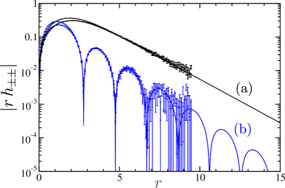
Figure 1: (color online) Pair distribution functions for the URPM at two state points on opposite sides of the Kirkwood line (see text for details), plotted as $|r\,h_{\pm\pm}|$ versus $r$ to illustrate the asymptotic behaviour. Lines are HNC, data points with error bars are MC. Lengths are expressed in units of $\sigma$.

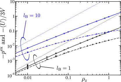
Figure 2: (color online) URPM thermodynamics along two isotherms showing $-p^{\mathrm{ex}}$ (solid HNC lines with square MC data points) and $-\langle U\rangle/3V$ (dashed HNC lines with diamond MC data points) as a function of density. The Debye-Hückel limiting law is shown as a dotted line in the two cases. Lengths and densities are expressed in units of $\sigma$, and thermodynamic quantities in units of $k_{\mathrm{B}}T/\sigma^{3}$.

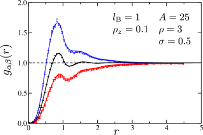
Figure 3: (color online) Pair distribution functions for a solvated model at the indicated state point. Lines are HNC, data points with error bars are MC. From top to bottom the curves are: $g_{+-}$; $g_{0+}=g_{0-}\approx g_{00}$; and $g_{++}=g_{--}$. The difference between $g_{0\pm}$ and $g_{00}$ is tiny and not resolved in this plot. Lengths and densities are expressed in units of $r_{c}$.

IV Results

IV.1 Comparison between HNC and MC

We first consider the URPM as a baseline. Fig. 1 shows the pair distribution functions plotted as $|r\,h(r)|$ at two state points on either side of the Kirkwood line: (a) $\rho_{z}\sigma^{3}=0.02$ and $l_{\mathrm{B}}/\sigma=1$ where the asymptotic decay is purely exponential; and (b) $\rho_{z}\sigma^{3}=0.2$ and $l_{\mathrm{B}}/\sigma=10$ where the decay is damped oscillatory. The agreement between HNC and MC is excellent. These MC simulations are expensive to perform even in the absence of a neutral solvent species. For (a) and (b) respectively, $10^{6}$ and $10^{5}$ MC configurations were required to reduce the errors to an acceptable level at large $r$ (note that there are ten times as many particles for the latter state point). A box of size $(20\sigma)^{3}$ is necessary to reach out to $r\approx 9\sigma$. Each state point required nearly 3000 hours of CPU time, in marked contrast to the HNC solution which takes less than a second. This is the origin of the claim earlier that HNC can be up to ten million times faster than MC.

MC simulation of the thermodynamics is much less demanding. Fig. 2 shows the excess pressure ($p^{\mathrm{ex}}=p-\rho k_{\mathrm{B}}T$) and internal energy for the URPM along isotherms at $l_{\mathrm{B}}/\sigma=1$ and 10. There is excellent quantitative agreement between HNC and MC. For the most part these simulations were carried out in a box of size $(10\sigma)^{3}$. For $l_{\mathrm{B}}/\sigma=1$ though we did check for finite size effects at the lowest investigated density by increasing the box size to $(15\sigma)^{3}$ and $(20\sigma)^{3}$. The results are shown in Fig. 2 as the multiple data points at $\rho_{z}\sigma^{3}=0.01$, and indicate that finite size effects are small.

The excess pressure and the internal energy (divided by three) are both expected to trend to the Debye-Hückel limiting law, $p^{\mathrm{ex}}=\langle U\rangle/3V=-k_{\mathrm{D}}^{3}/(24\pi)$, as the density decreases. As can be seen, the approach is rather slow. Note that the relation $p^{\mathrm{ex}}=\langle U\rangle/3V$ is a consequence of Clausius’ virial theorem applied to point particles interacting with the Coulomb potential Clausius (1870).

In the presence of a neutral solvent the attainable MC accuracy is much diminished, largely because of the need to equilibrate the solvent particles. Fig. 3 shows an example of pair distribution functions for a solvated model at a typical state point. Again there is excellent agreement between HNC and MC (box size $(10r_{c})^{3}$). In this plot note that symmetry enforces $g_{0+}=g_{0-}$ and $g_{++}=g_{--}$. The approximate symmetry $g_{0\pm}\approx g_{00}$ is only very weakly broken in HNC (and not at all in the RPA) since it is exactly true that $U_{0\pm}=U_{00}$.

To summarise the key result of this section: HNC accurately reproduces MC for the parameter ranges of interest. Thus we conclude that we can place enough confidence in HNC to use it as a tool to explore the properties of the model.

Figure 4: Total correlation function $h_{++}(r)$ from HNC for the URPM at $l_{\mathrm{B}}=1$ and $\rho_{z}=0.01(1)5$ (top to bottom). Curves have been displaced for clarity. The Kirkwood transition from pure exponential decay ($\rho_{z}\lesssim 0.03$) to damped oscillatory ($\rho_{z}\gtrsim 0.03$) is clearly seen. Lengths and densities are expressed in units of $\sigma$.

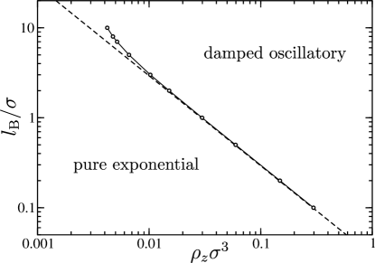
Figure 5: The Kirkwood line for the URPM. The solid line with circles is from HNC. The dashed line is the RPA, from Eq. (12). If solvent particles and short range repulsions are added, this map is practically unchanged.

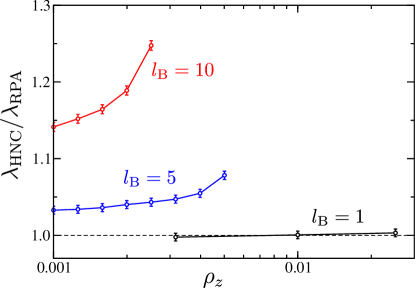
Figure 6: (color online) The screening length for the URPM, comparing the value extracted by fitting the asymptotic tails of $h_{\alpha\beta}$ in HNC, to the RPA value from Eq. (11). Lengths and densities are expressed in units of $\sigma$.

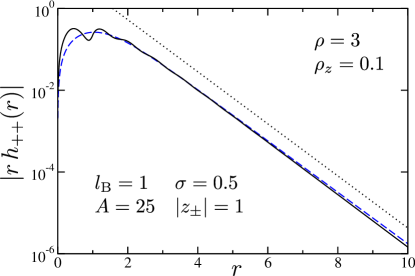
Figure 7: (color online) Comparison between a fully solvated model (solid line, black) and the URPM equivalent (dashed line, blue). Both are calculated using HNC. The dotted line is the RPA prediction from Eq. (11). Lengths and densities are expressed in units of $r_{c}$.

IV.2 Screening properties from HNC

We now use the HNC to calculate the screening length from the asymptotic behaviour of the computed total correlation functions, focussing at first on the URPM. Fig. 4 shows the typical behaviour of $h_{++}(r)$ through the Kirkwood transition as $\rho_{z}$ varies at fixed $l_{\mathrm{B}}$. Note that the decay rate of the total correlation function at first increases with increasing density, until one crosses the Kirkwood line, after which the decay rate remains roughly constant but the period of the oscillations decreases. This behaviour is similar to the RPA, and presumably reflects the pole structure as discussed in section III.3.

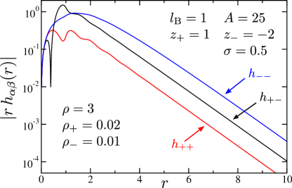
Figure 8: (color online) HNC results for a 1:2 electrolyte. Lengths and densities are expressed in units of $r_{c}$.

One can ‘zero in’ on the Kirkwood line transition by systematically narrowing the range of densities which are plotted. In this case one finds the transition is located at $\rho_{z}\sigma^{3}\approx(30.0\pm 0.5)\times 10^{-3}$. By proceeding in this way, the entire Kirkwood line can be mapped out in the $(\rho_{z}\sigma^{3},l_{\mathrm{B}}/\sigma)$ plane. This is shown in Fig. 5, where HNC is compared to the RPA Kirkwood line from Eq. (12). We see that for $l_{\mathrm{B}}/\sigma\lesssim 5$ the RPA is practically indistinguishable from HNC, and even at $l_{\mathrm{B}}/\sigma=10$ the difference is still less than 40%. Above this value of $l_{\mathrm{B}}/\sigma$ HNC ceases to converge to a solution.

On the low density side of the Kirkwood line the HNC screening length can be found by fitting the tail of total correlation function to the expected asymptotic behaviour in Eq. (4). Results along isotherms at three values of $l_{\mathrm{B}}/\sigma$ are shown in Fig. 6. Crucially, we see that for $l_{\mathrm{B}}/\sigma\lesssim 5$, the RPA screening length from Eq. (11) is in error by less than 10% compared to HNC.

All the results presented so far have been for the URPM in the absence of a neutral solvent species. Remarkably, we have found that very little changes if short range repulsions are added ($A=25$) and a solvent is included ($\rho r_{c}^{3}=3$). For example the Kirkwood line in Fig. 5 is practically unchanged and we have found the same to be true for the screening length itself. We give a single example here. Fig. 7 shows the asymptotic decay of $h_{++}(r)$ for the indicated state point for a fully solvated model, compared to the equivalent URPM at $l_{\mathrm{B}}/\sigma=2$ and $\rho_{z}\sigma^{3}=0.0125$. A line indicating the RPA decay from Eq. (11) is also included. We see that the presence of a solvent and short range repulsions confers some liquid structure at short distances but the asymptotic decay is practically unchanged, and agrees well with the RPA.

Lastly we turn to the more complicated case of an asymmetric electrolyte. Fig. 8 shows the total correlation functions for a 1:2 electrolyte calculated using HNC. As can be seen the asymmetry splits apart the three ionic correlation functions, but nevertheless they share a common decay length, $\lambda_{\mathrm{HNC}}/r_{c}\approx 0.93$. This can be compared to $\lambda_{\mathrm{RPA}}/r_{c}\approx 1.02$, calculated from Eq. (11) using $\rho_{z}r_{c}^{3}=0.06$ (i. e. $\rho_{z}=\rho_{+}+4\rho_{-}$). The difference between HNC and RPA is less than 10%, as might be expected from Fig. 6 since the 1:2 case is intermediate between the 1:1 case ($l_{\mathrm{B}}/\sigma=2$) and the 2:2 case ($l_{\mathrm{B}}/\sigma=8$).

The main conclusions from this section are: first the solvent has practically no effect on the screening properties so that Fig. 5 can be used as a quasi-universal quide, and second for many applications, such as to 1:1 electrolytes, the RPA suffices.

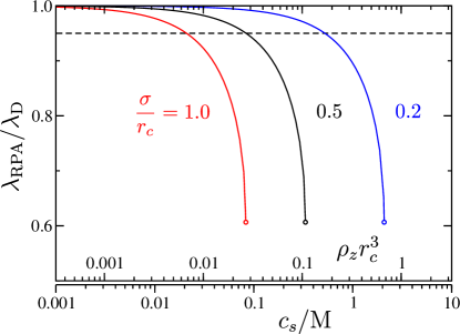
Figure 9: (color online) Ratio between RPA screening length and Debye length for a 1:1 electrolyte, as a function of concentration, for three choices of $\sigma$. The lower (upper) horizontal axis shows the concentration in physical (simulation) units. Each curve terminates when the model system crosses the Kirkwood line. The dashed line is at $\lambda_{\mathrm{RPA}}/\lambda_{\mathrm{D}}=0.95$.

1	$l_{\mathrm{B}}/r_{c}$	1.090
2	$\rho_{z}r_{c}^{3}$	0.032
3	$\lambda_{\mathrm{D}}/r_{c}$	1.500
4	$\sigma/r_{c}$	$-$0.500	$-$1.00
5	$l_{\mathrm{B}}/\sigma$	$-$2.170	$-$1.09
6	$4\pi el_{\mathrm{B}}\rho_{z}\sigma^{2}$	$-$0.300	$-$1.20
7	$W_{0}(-4\pi l_{\mathrm{B}}\rho_{z}\sigma^{2})$	$-0.125$	$-0.88\pm 0.60\,i$
8	$\lambda_{\mathrm{RPA}}/r_{c}$	$-$1.410	$-$—
9	$\lambda_{\mathrm{RPA}}/\lambda_{\mathrm{D}}$	$-$0.940	$-$—

Table 1: Sample calculation for a $0.1\,\mathrm{M}$ 1:1 electrolyte.

IV.3 Worked example

Let us work through the example given at the end of section III.2, for which the RPA solution is applicable. The calculations are shown in the numbered rows in Table 1. We start from the standard DPD mapping with $r_{c}=0.645\,\mathrm{nm}$ and $l_{\mathrm{B}}=0.7\,\mathrm{nm}$. This gives $l_{\mathrm{B}}/r_{c}=1.09$ (row 1). If the molar concentration of a 1:1 electrolyte is $c_{s}$, then $\rho_{z}=2\times 10^{3}c_{s}N_{A}$ (row 2; the factor two accounts for both species of ion). The Debye length (row 3) follows from Eq. (5), here in the form $\lambda_{\mathrm{D}}=(4\pi l_{\mathrm{B}}\rho_{z})^{-1/2}$. Alternatively one can use the well known expression $\lambda_{\mathrm{D}}=0.31\,\mathrm{nm}/\sqrt{c_{s}}$ from the colloidal literature Verwey and Overbeek (1948). We choose a value for $\sigma$ (row 4) and calculate the left hand side of the inequality in Eq. (12) (row 6). For the choice $\sigma=r_{c}/2$, Eq. (12) is satisfied and we are on the low density side of the Kirkwood line. We can then use the value of the Lambert function (row 7) to calculate $\lambda_{\mathrm{RPA}}$ (row 8) from Eq. (11). Given that $l_{\mathrm{B}}/\sigma\lesssim 5$ (row 5), this should be a good estimate of the true screening length. As claimed in section III.2, the answer deviates from the Debye length by only 6% (row 9). For the choice $\sigma=r_{c}$ though, Eq. (12) is violated (row 6), and we are on the high density side of the Kirkwood line. This is also indicated by the fact that the Lambert function (row 7) evaluates to a complex number.

IV.4 The choice of $\sigma$

As we have seen, a mapping to a physical system fixes $l_{\mathrm{B}}$ and $r_{c}$, but the choice of $\sigma$ remains unresolved. Our study so far reveals this choice is a balance of conflicting requirements. On the one hand we would like to increase $\sigma$ as much as possible, mainly because this reduces the cost of computing the electrostatic interactions in a simulation. On the other hand if $\sigma$ is too large we run the risk of deviating strongly from the expected screening properties of the physical system, and may ultimately cross the Kirkwood line in Fig. 5. Such behaviour is almost certain to be artefactual since the chances of coinciding with similar behaviour in the physical system seem remote.

For example for a 1:1 aqueous electrolyte we can plot the ratio $\lambda_{\mathrm{RPA}}/\lambda_{\mathrm{D}}$ as a function of salt concentration $c_{s}$, using the method just described in section IV.3. Fig. 9 shows just such a plot, for three choices of $\sigma/r_{c}$. Inspection suggests as sensible compromise might be $\sigma/r_{c}=0.5$, since this restricts significant deviations from the Debye length (i. e. more than 10%) to $c_{s}\gtrsim 0.15\,\mathrm{M}$, where in any case the Debye length is starting to become comparable to $r_{c}$.

V Discussion

Let us close with some more remarks about implementation, and indicate avenues for future work. First, let us dispose of an elementary point. The simulations described here have been performed using MC, rather than DPD. The reason for this is that we are interested in equilibrium properties, and MC is free from issues such as the choice of integration algorithm and time step Groot and Warren (1997). Nevertheless the Ewald method can easily be applied to a dynamical simulation, by calculating the forces that arise from the potential energy in Eq. (13).

The usual Ewald implementation for point charges introduces a ‘splitting parameter’ so that part of the interaction is calculated in real space and part in reciprocal space Allen and Tildesley (1987). Here we have ‘physical-ised’ the splitting parameter by linking it to the Gaussian charge size $\sigma$, so that we can discard the real-space interaction. This may not always be the best choice, since one cannot then optimise the splitting parameter to match the simulation box size Frenkel and Smit (2002). However Coslovich et al. found that there is practically no benefit in divorcing the splitting parameter from the Gaussian charge size, at least for the URPM for their parameter ranges. Nevertheless it is worth bearing in mind this possibility, particularly if $\sigma$ is much smaller than the simulation box size.

Aside from standard Ewald, any existing molecular dynamics (MD) method could be used in principle to calculate electrostatic interactions in DPD. Most notable are the P3M (particle-particle-particle-mesh) methods, such as that introduced by Groot Groot (2003), and hybrids such as smooth particle mesh Ewald Essmann et al. (1995). Some of these methods are highly parallelisable Beckers et al. (1998), or highly efficient in other ways Essmann et al. (1995). These MD methods are typically developed for point charges, but the application to smeared charges should involve a straightforward extension to the underlying algorithms.

As mentioned in the introduction, there is no consensus on the best form of charge smearing (linear, exponential, Gaussian, et c.), nor, perhaps, does there need to be. All smearing methods generate pair potentials which may differ in the short range part, but share a common $l_{\mathrm{B}}/r$ dependence for large $r$. This raises the question of whether the methods can be mapped on to one another, vis à vis the screening properties. Related to this is our observation that short range repulsions have practically no effect on the screening properties. Whilst this is a great bonus for applications, it cannot hold generally, for it would imply that there should be negligible effect of the choice of smearing. But we know this is manifestly untrue: two Gaussian charge models with $\sigma^{\prime}\neq\sigma$ do not have the same screening properties. More generally, in any smeared charge model, another length scale must be present to non-dimensionalise $l_{\mathrm{B}}$. The question of how to determine this length scale remains unsolved. Our present results suggest that a systematic use of HNC could give an answer, thus providing a ‘Rosetta Stone’ tying together the existing treatments of DPD electrostatics. This is the subject of ongoing investigations.

Separate from this, a long term goal is to incorporate specific ion effects into the model, such as the Hofmeister series Collins and Washabaugh (1985). As mentioned in section II, we have here focussed on a constant repulsion amplitude matrix $A_{ij}=A$. Obviously there is scope to go beyond this, using HNC to calculate both the structural and thermodynamic consequences of unequal repulsion amplitudes. The hope is that a suitable choice of $A_{ij}$ can be found, which will systematically and transferrably capture specific ion effects. It is encouraging to note in this respect that a similar programme has been pursued with some success recently, for MD Kalcher and Dzubiella (2009); Vrbka et al. (2009).

References

- Frenkel and Smit (2002) D. Frenkel and B. Smit, Understanding molecular simulation (Academic Press, San Diego, 2002).
- Noro et al. (2003) M. G. Noro, F. Meneghini, and P. B. Warren, ACS Symp. series 861, 242 (2003).
- Groot and Warren (1997) R. D. Groot and P. B. Warren, J. Chem. Phys. 107, 4423 (1997).
- Groot and Madden (1998) R. D. Groot and T. J. Madden, J. Chem. Phys. 108, 8713 (1998).
- Spenley (2000) N. A. Spenley, Europhys. Lett. 49, 534 (2000).
- Sultan et al. (2010) E. Sultan, J.-W. van de Meent, E. Somfai, A. N. Morozov, and W. van Saarloos, EPL 90, 64002 (2010).
- Prinsen et al. (2002) P. Prinsen, P. B. Warren, and M. A. J. Michels, Phys. Rev. Lett. 89, 148302 (2002).
- Groot and Rabone (2001) R. D. Groot and K. L. Rabone, Biophys. J. 81, 725 (2001).
- Shillcock and Lipowsky (2002) J. C. Shillcock and R. Lipowsky, J. Chem. Phys. 117, 5048 (2002).
- Boek et al. (1997) E. S. Boek, P. V. Coveney, H. N. W. Lekkerkerker, and P. van der Schoot, Phys. Rev. E 55, 3124 (1997).
- Groot (2003) R. D. Groot, J. Chem. Phys. 118, 11265 (2003).
- Fisher and Ruelle (1966) M. E. Fisher and D. Ruelle, J. Math. Phys. 7, 260 (1966).
- González-Melchor et al. (2006) M. González-Melchor, E. Mayoral, M. E. Velázquez, and J. Alejandre, J. Chem. Phys. 125, 224107 (2006).
- Coslovich et al. (2011a) D. Coslovich, J.-P. Hansen, and G. Kahl, Soft Matter 7, 1690 (2011a).
- Coslovich et al. (2011b) D. Coslovich, J.-P. Hansen, and G. Kahl, J. Chem. Phys. 134, 244514 (2011b).
- Nikoubashman et al. (2012) A. Nikoubashman, J.-P. Hansen, and G. Kahl, J. Chem. Phys. 137, 094905 (2012).
- (17) See http://sunlightdpd.sourceforge.net/.
- Warren and Masters (2013) P. B. Warren and A. J. Masters, J. Chem. Phys. 138, 074901 (2013).
- Kirkwood (1936) J. G. Kirkwood, Chem. Rev. 19, 275 (1936).
- Fisher and Widom (1969) M. E. Fisher and B. Widom, J. Chem. Phys. 50, 3756 (1969).
- Hansen and McDonald (2006) J.-P. Hansen and I. R. McDonald, Theory of simple liquids (Academic Press, Amsterdam, 2006).
- Ng (1974) K.-C. Ng, J. Chem. Phys. 61, 2680 (1974).
- Kelley and Montgomery Pettitt (2004) C. T. Kelley and B. Montgomery Pettitt, J. Comp. Phys. 197, 491 (2004).
- Vrbka et al. (2009) L. Vrbka, M. Lund, I. Kalcher, J. Dzubiella, R. R. Netz, and W. Kunz, J. Chem. Phys. 131, 154109 (2009).
- Hopkins et al. (2006) P. Hopkins, A. J. Archer, and R. Evans, J. Chem. Phys. 124, 054503 (2006).
- Corless et al. (1996) R. M. Corless, G. H. Gonnet, D. E. G. Hare, D. J. Jeffrey, and D. E. Knuth, Adv. Comput. Math. 5, 329 (1996).
- (27) The Lambert function can be found in commercial packages such as Mathematica and MATLAB, in open source packages such as Maxima and Octave, in the R statistical platform, and in the GNU Scientific Library. One-off evaluations can be performed on the internet using the Wolfram Alpha computational knowledge engine, e. g. enter ‘LambertW[-0.11]’ for the result in row 7 in Table 1.
- Allen and Tildesley (1987) M. P. Allen and D. J. Tildesley, Computer simulation of liquids (Clarendon, Oxford, UK, 1987).
- (29) See W. Smith, “Coping with the pressure! – how to calculate the virial”, CCP5 Newsletter No. 26 (1987); currently available at ftp://ftp.dl.ac.uk/ccp5.newsletter/26/.
- Clausius (1870) R. J. E. Clausius, Phil. Mag. 40, 122 (1870).
- Verwey and Overbeek (1948) E. J. W. Verwey and J. Th. G. Overbeek, Theory of the stability of lyophobic colloids (Elsevier, Amsterdam, 1948).
- Essmann et al. (1995) U. Essmann, L. Perera, M. L. Berkowitz, T. Darden, H. Lee, and L. G. Pedersen, J. Chem. Phys. 103, 8577 (1995).
- Beckers et al. (1998) J. V. L. Beckers, C. P. Lowe, and S. W. de Leeuw, Mol. Sim. 20, 369 (1998).
- Collins and Washabaugh (1985) K. D. Collins and M. W. Washabaugh, Quart. Rev. Biophys. 18, 323 (1985).
- Kalcher and Dzubiella (2009) I. Kalcher and J. Dzubiella, J. Chem. Phys. 130, 134507 (2009).