Set-Membership Conjugate Gradient Constrained Adaptive Filtering Algorithm for Beamforming

Abstract

We introduce a new linearly constrained minimum variance (LCMV) beamformer that combines the set-membership (SM) technique with the conjugate gradient (CG) method, and develop a low-complexity adaptive filtering algorithm for beamforming. The proposed algorithm utilizes a CG-based vector and a variable forgetting factor to perform the data-selective updates that are controlled by a time-varying bound related to the parameters. For the update, the CG-based vector is calculated iteratively (one iteration per update) to obtain the filter parameters and to avoid the matrix inversion. The resulting iterations construct a space of feasible solutions that satisfy the constraints of the LCMV optimization problem. The proposed algorithm reduces the computational complexity significantly and shows an enhanced convergence and tracking performance over existing algorithms.

Key words — Set-membership filtering, conjugate gradient algorithms, adaptive algorithms, beamforming.

1 Introduction

Beamforming is an ubiquitous task in adaptive filtering and array signal processing problems, and has been found widespread applications in radar, sonar and wireless communications. Among the existing techniques, the most promising one is the optimal linearly constrained minimum variance (LCMV) beamformer [1] due to its simplicity and effectiveness. The LCMV beamformer aims to suppress interference at the array output while improving the reception of the desired signal. The constraint corresponds to prior knowledge of the array response of the desired user $\boldsymbol{a}(\theta_{0})\in\mathbb{C}^{m\times 1}$, where $\theta_{0}$ is the direction of arrival (DOA) of the desired signal and $m$ is the number of sensor elements in the array.

The optimal LCMV beamformer requires the computation of the inverse of the covariance matrix $\boldsymbol{R}=\mathbb{E}[\boldsymbol{r}\boldsymbol{r}^{H}]\in\mathbb{C}^{m\times m}$ with $\boldsymbol{r}\in\mathbb{C}^{m\times 1}$ being the received vector, and results in a heavy computational load. Many adaptive filtering algorithms have been reported to realize the beamformer design efficiently. The well-known adaptive algorithms include stochastic gradient (SG), recursive least squares (RLS), affine projection (AP), and conjugate gradient (CG) [2]-[6]. The SG algorithm is simple to implement but suffers from a slow convergence rate and the misadjustment. The RLS algorithm enjoys fast convergence but is more complex to implement and may become unstable due to the divergence problem and numerical problems [2]. The AP algorithm requires the inversion of a matrix whose dimension is given by the projection order, which results in a heavy computational load of the AP algorithm if chosen as a large number. Besides, the convergence of the AP algorithm is often much slower than the RLS. The CG algorithm has a good tradeoff between performance and complexity since it has a faster convergence rate than the SG and AP algorithms, and requires a lower computational cost when compared with the RLS algorithm. Many adaptive CG algorithms have been reported in [4]-[6], and the references therein. Modified CG versions based on the LCMV criterion can be found in [7], whereas for other subspace-based algorithms the reader is referred to [8]-[14].

In this paper, we introduce a more economic adaptive algorithm based on the CG method for the LCMV beamformer design. The proposed algorithm utilizes the set-membership (SM) technique [15], [18] to enforce the constraints and to reduce the computational complexity significantly without performance degradation. The SM specifies a bound on the magnitude of the array output and performs data-selective updates to estimate the filter parameters. It involves two steps: 1) information evaluation and 2) parameter update. If step 2) does not occur frequently, and step 1) does not require much complexity, the overall complexity can be saved substantially. SM algorithms based on the SG and RLS methods have been reported in [15]-[19]. Here, we use the SM technique in the CG algorithm that was reported in [7], and develop a new adaptive algorithm, which is termed SM-CG. Specifically, we define a new LCMV optimization problem related to a constraint on the bound of the array output, and perform the filter optimization to calculate the solution. A parameter dependent time-varying bound is employed to measure the quality of the filter parameters that could satisfy the constraints and to improve the tracking performance in dynamic scenarios. The parameters are only updated if the bounded constraint cannot be satisfied. For the update, we define a new CG-based vector $\boldsymbol{v}\in\mathbb{C}^{m\times 1}$ to create a relation with $\boldsymbol{R}$ and $\boldsymbol{a}(\theta_{0})$, namely, $\boldsymbol{v}=\boldsymbol{R}^{-1}\boldsymbol{a}(\theta_{0})$. The proposed algorithm calculates $\boldsymbol{v}$ via one iteration per update to obtain filter parameters without the matrix inverse. The updated parameters are encompassed in a parameter space, in which each member is consistent with the bounded constraint and the constraint on the array response based on the optimization problem. Compared with the existing algorithms, the proposed algorithm exhibits an enhanced convergence and tracking performance with relatively low computational complexity. Simulation results illustrate the performance of the proposed SM-CG algorithm.

2 System Model and Beamformer Design

Let us suppose that $q$ narrowband signals impinge on a uniform linear array (ULA) of $m$ ($q\leq m$) sensor elements. The sources are assumed to be in the far field with DOAs $\theta_{0}$, …, $\theta_{q-1}$. The received vector $\boldsymbol{r}$ can be modeled as

$$\centering{\boldsymbol{r}}={\boldsymbol{A}}({\boldsymbol{\theta}}){\boldsymbol{s}}+{\boldsymbol{n}},\@add@centering$$ (1)

where $\boldsymbol{\theta}=[\theta_{0},\ldots,\theta_{q-1}]^{T}\in\mathbb{R}^{q\times 1}$ is the DOAs, ${\boldsymbol{A}}({\boldsymbol{\theta}})=[{\boldsymbol{a}}(\theta_{0}),\ldots,{\boldsymbol{a}}(\theta_{q-1})]\in\mathbb{C}^{m\times q}$ composes the steering vectors ${\boldsymbol{a}}(\theta_{k})=[1,e^{-2\pi j\frac{d}{\lambda_{c}}cos{\theta_{k}}},\ldots,e^{-2\pi j(m-1)\frac{d}{\lambda_{c}}cos{\theta_{k}}}]^{T}\in\mathbb{C}^{m\times 1},~{}~{}~{}(k=0,\ldots,q-1)$, where $\lambda_{c}$ is the wavelength and $d=\lambda_{c}/2$ is the inter-element distance of the ULA, and to avoid mathematical ambiguities, the steering vectors $\boldsymbol{a}(\theta_{k})$ are considered to be linearly independent, ${\boldsymbol{s}}\in\mathbb{C}^{q\times 1}$ is the source data, ${\boldsymbol{n}}\in\mathbb{C}^{m\times 1}$ is the white Gaussian noise, and $(\cdot)^{T}$ stands for the transpose. The output of a narrowband beamformer is

$$\centering y={\boldsymbol{w}}^{H}{\boldsymbol{r}},\@add@centering$$ (2)

where ${\boldsymbol{w}}=[w_{1},\ldots,w_{m}]^{T}\in\mathbb{C}^{m\times 1}$ is the complex weight vector of the adaptive filter, and $(\cdot)^{H}$ stands for the Hermitian transpose. For the optimal LCMV beamformer, the aim is to solve the optimization problem

$$\begin{split}\textrm{min}~{}\mathbb{E}[|y|^{2}]&=\boldsymbol{w}^{H}\boldsymbol{R}\boldsymbol{w}\\ {\rm subject~{}to}~{}~{}~{}\boldsymbol{w}^{H}\boldsymbol{a}(\theta_{0}&)=\gamma,\end{split}$$ (3)

where $\gamma$ is a constant, and $\boldsymbol{R}$ is the covariance matrix of the received vector. The solution of (3) is $\boldsymbol{w}_{\textrm{opt}}=\frac{\gamma\boldsymbol{R}^{-1}\boldsymbol{a}(\theta_{0})}{\boldsymbol{a}^{H}(\theta_{0})\boldsymbol{R}^{-1}\boldsymbol{a}(\theta_{0})}$. The SG, RLS, AP, and CG algorithms have been employed to realize the design in different ways. Among them, the CG-based algorithms exhibit some advantages due to their attractive tradeoff between performance and complexity.

3 Proposed SM-CG Algorithm

In this section, we introduce a new constrained optimization strategy that combines the SM technique with the LCMV design and utilizes the CG-based adaptive filtering algorithm.

3.1 Time-varying SM-CG scheme

In the proposed scheme depicted in Fig. 1, the received vector $\boldsymbol{r}(i)$ is processed at time instant $i$ by the LCMV filter controlled by the adaptive CG algorithm to generate the output $y(i)$. For the existing CG algorithms [4]-[5], it is necessary to update ${\boldsymbol{w}}(i)$ for each time instant $i$ with many iterations to obtain a good performance. In the proposed scheme, the SM technique is embedded to specify a time-varying bound $\delta(i)$ on the amplitude of $y(i)$. The update only performs if the bounded constraint $|y(i)|^{2}\leq|\delta(i)|^{2}$ cannot be satisfied. For each update, some valid estimates of ${\boldsymbol{w}}(i)$ satisfy the bound. Thus, the solution to the proposed scheme is a set in the parameter space.

Fig. 1: Proposed SM-CG structure

The time-varying bound $\delta(i)$ is a unique coefficient for the proposed scheme to check if the update is carried out or not. It is better if $\delta(i)$ could reflect the characteristics of the environment since it benefits the tracking of the proposed algorithm. We introduce a parameter dependent bound (PDB) that is similar to the work in [20] and involves the evolution of ${\boldsymbol{w}}(i)$ obtained from the proposed algorithm. The time-varying bound is

$$\delta(i)=\beta\delta(i-1)+(1-\beta)\sqrt{\alpha\|\boldsymbol{w}(i-1)\|^{2}\hat{\sigma}_{n}^{2}(i)},$$ (4)

where $\beta$ is a forgetting factor that should be set to guarantee a proper time-averaged estimate of the evolutions of $\boldsymbol{w}(i-1)$, $\alpha$ ($\alpha>1$) is a tuning coefficient that impacts the update rate and convergence, and $\hat{\sigma}_{n}^{2}(i)$ is an estimate of the noise power, which is assumed to be known at the receiver. The term $\|\boldsymbol{w}(i-1)\|^{2}\hat{\sigma}_{n}^{2}(i)$ is the variance of the inner product of the weight vector with the noise that provides information on the evolution of $\boldsymbol{w}(i-1)$. The time-varying bound provides a smoother evolution of the weight vector trajectory and thus avoids too high or low values of the squared norm of $\boldsymbol{w}$. The proposed SM-CG scheme utilizes the time-varying bound to create a relation between the estimated parameters and the environment.

According to $\delta(i)$, we define $\mathcal{H}_{i}$ to be the set containing all the estimates of $\boldsymbol{w}(i)$ for which the associated array output at time instant $i$ is consistent with the bound, which is given by $\mathcal{H}_{i}=\big{\{}\boldsymbol{w}(i)\in\mathbb{C}^{m\times 1}:|y(i)|^{2}\leq\delta^{2}(i)\big{\}}$. The set $\mathcal{H}_{i}$ is referred to as the constraint set, and its boundaries are hyperplanes. Then, we define the exact feasibility set $\Theta_{i}$ to be the intersection of the constraint sets over the instants $l=1,\ldots,i$, which is

$$\Theta_{i}=\mathop{\bigcap_{{l=1}}}_{(s_{0},\boldsymbol{r})\in\boldsymbol{S}}^{i}\mathcal{H}_{l},$$ (5)

where $s_{0}(i)$ is the transmitted data of the desired user and $\boldsymbol{S}$ is the set including all possible data pairs $\{s_{0}(i),{\boldsymbol{r}}(i)\}$. It is clear that $\Theta$ should encompass all the solutions that satisfy the bounded constraint until $i\rightarrow\infty$. In practice, $\boldsymbol{S}$ cannot be traversed all over. Therefore, we define a more practical set (membership set) $\Psi_{i}=\bigcap_{l=1}^{i}\mathcal{H}_{l}$ instead. The membership set is a limiting set of the feasibility set. They are equal if the data pairs traverse $\boldsymbol{S}$ completely.

3.2 Proposed SM-CG Adaptive Algorithm

We derive a new adaptive algorithm based on the SM-CG scheme. It begins with an LCMV optimization problem that incorporates the constraint on the bound of the array output:

$$\begin{split}&\textrm{minimize}~{}~{}\mathbb{E}[|\boldsymbol{w}^{H}\boldsymbol{r}(i)|^{2}]=\boldsymbol{w}^{H}\boldsymbol{R}\boldsymbol{w}\\ &\textrm{subject~{}to}~{}~{}\boldsymbol{w}^{H}\boldsymbol{a}(\theta_{0})=\gamma~{}\textrm{and}~{}{|y(i)|}^{2}=\delta^{2}(i),\end{split}$$ (6)

where $\delta(i)$ determines a set of solutions of $\boldsymbol{w}$ within the constraint set $\mathcal{H}$ with respect to each time instant.

The constrained optimization problem can be transformed into an unconstrained one by the method of Lagrange multipliers. The Lagrangian is given by

$$\begin{split}&J({\boldsymbol{w}}(i))=\sum_{l=1}^{i-1}\lambda_{1}^{i-l}(i)\boldsymbol{w}^{H}(i)\boldsymbol{r}(l)\boldsymbol{r}^{H}(l)\boldsymbol{w}(i)\\ &+2\lambda_{1}(i)\mathfrak{R}\big{\{}|\boldsymbol{w}^{H}(i)\boldsymbol{r}(i)|^{2}-\delta^{2}(i)\big{\}}+2\lambda_{2}\mathfrak{R}\big{\{}\boldsymbol{w}^{H}(i)\boldsymbol{a}(\theta_{0})-\gamma\big{\}},\end{split}$$ (7)

where $\mathfrak{R}\{\cdot\}$ selects the real part of the quantity, $\lambda_{1}(i)$ plays the role of the forgetting factor and Lagrange multiplier with respect to the bounded constraint and is calculated only if the bounded constraint cannot be satisfied. The scalar $\lambda_{2}$ is another Lagrange multiplier to ensure the constraint on the steering vector of the desired user.

Using the assumption, computing the gradient of $\boldsymbol{w}(i)$ with respect to (7) and equating it to a null vector, we have

$$\boldsymbol{w}(i)=\frac{\gamma\hat{\boldsymbol{R}}^{-1}(i)\boldsymbol{a}(\theta_{0})}{\boldsymbol{a}^{H}(\theta_{0})\hat{\boldsymbol{R}}^{-1}(i)\boldsymbol{a}(\theta_{0})},$$ (8)

where $\hat{\boldsymbol{R}}(i)=\hat{\boldsymbol{R}}(i-1)+\lambda_{1}(i)\boldsymbol{r}(i)\boldsymbol{r}^{H}(i)$ can be regarded as an alternative form to estimate the covariance matrix $\boldsymbol{R}$.

To calculate $\boldsymbol{w}(i)$ efficiently, we adopt the CG-based adaptive algorithm due to its attractive tradeoff between performance and complexity. Specifically, we define a CG-based vector $\boldsymbol{v}(i)=\hat{\boldsymbol{R}}^{-1}\boldsymbol{a}(\theta_{0})$ and use an iterative way to calculate it. The resulting solution can be written as

$$\boldsymbol{w}(i)=\frac{\gamma\boldsymbol{v}(i)}{\boldsymbol{a}^{H}(\theta_{0})\boldsymbol{v}(i)},$$ (9)

where $\boldsymbol{v}(i)$ is viewed as an intermediate weight vector for enforcing the constraints and avoiding the matrix inverse. In the following, we describe a simple CG procedure with only one iteration per update to calculate $\boldsymbol{v}(i)$ for computing ${\boldsymbol{w}}(i)$.

The CG-based vector is expressed by

$$\boldsymbol{v}(i)=\boldsymbol{v}(i-1)+\alpha(i)\boldsymbol{p}(i),$$ (10)

where $\boldsymbol{p}(i)$ is the direction vector and $\alpha(i)$ is the corresponding coefficient.

The direction vector $\boldsymbol{p}(i)$ is obtained by a linear combination of the previous direction vector and the negative gradient vector $\boldsymbol{g}(i)=\boldsymbol{a}(\theta_{0})-\hat{\boldsymbol{R}}(i)\boldsymbol{v}(i)$ of $J(\boldsymbol{v}(i))=\boldsymbol{v}^{H}(i)\hat{\boldsymbol{R}}(i)\boldsymbol{v}(i)-2\Re\{\boldsymbol{v}^{H}(i)\boldsymbol{a}(\theta_{0})\}$ [7], which is

$$\boldsymbol{p}(i+1)=\boldsymbol{g}(i)+\beta(i)\boldsymbol{p}(i),$$ (11)

where $\beta(i)$ is chosen to provide conjugacy [5] for the direction vectors.

In order to derive the coefficients $\alpha(i)$ and $\beta(i)$, we consider a recursive form of $\boldsymbol{g}(i)$

$$\boldsymbol{g}(i)=\boldsymbol{g}(i-1)-\alpha(i)\hat{\boldsymbol{R}}(i)\boldsymbol{p}(i)-\lambda_{1}(i)\boldsymbol{r}(i)\boldsymbol{r}^{H}(i)\boldsymbol{v}(i-1).$$ (12)

From [5], the coefficient $\alpha(i)$ should satisfy the convergence bound $0\leq\boldsymbol{p}^{H}(i)\boldsymbol{g}(i)\leq 0.5\boldsymbol{p}^{H}(i)\boldsymbol{g}(i-1)$ [5]. According to this bound, premultiplying (12) with $\boldsymbol{p}^{H}(i)$ and making a rearrangement, we have

$$\begin{split}&\frac{0.5\boldsymbol{p}^{H}(i)\boldsymbol{g}(i-1)-\lambda_{1}(i)\boldsymbol{p}^{H}(i)\boldsymbol{r}(i)\boldsymbol{r}^{H}(i)\boldsymbol{v}(i-1)}{\boldsymbol{p}^{H}(i)\hat{\boldsymbol{R}}(i)\boldsymbol{p}(i)}\leq\\ &\alpha(i)\leq\frac{\boldsymbol{p}^{H}(i)\boldsymbol{g}(i)-\lambda_{1}(i)\boldsymbol{p}^{H}(i)\boldsymbol{r}(i)\boldsymbol{r}^{H}(i)\boldsymbol{v}(i-1)}{\boldsymbol{p}^{H}(i)\hat{\boldsymbol{R}}(i)\boldsymbol{p}(i)}.\end{split}$$ (13)

The relations in (13) are satisfied if $\alpha(i)$ is

$$\alpha(i)=\frac{(1-\eta)\boldsymbol{p}^{H}(i)\boldsymbol{g}(i-1)-\lambda_{1}(i)\boldsymbol{p}^{H}(i)\boldsymbol{r}(i)\boldsymbol{r}^{H}(i)\boldsymbol{v}(i-1)}{\boldsymbol{p}^{H}(i)\hat{\boldsymbol{R}}(i)\boldsymbol{p}(i)},$$ (14)

where $0\leq\eta\leq 0.5$.

For $\beta(i)$, since $\boldsymbol{p}^{H}(i)\hat{\boldsymbol{R}}(i)\boldsymbol{p}(i+1)=0$, it follows that

$$\beta(i)=-\frac{\boldsymbol{p}^{H}(i)\hat{\boldsymbol{R}}(i)\boldsymbol{g}(i)}{\boldsymbol{p}^{H}(i)\hat{\boldsymbol{R}}(i)\boldsymbol{p}(i)}.$$ (15)

The coefficient $\lambda_{1}(i)$ is important to obtain the filter parameters. The SM technique provides an adaptive strategy to obtain it following the changes of the scenarios. Substituting (10) and (14) into the bounded constraint in (6) and performing some algebraic manipulations, we obtain

$$\lambda_{1}(i)=\frac{\lambda_{11}(i)-\lambda_{12}(i)}{\lambda_{13}(i)-\lambda_{14}(i)},$$ (16)

where
$\lambda_{11}(i)=\tau_{1}(i)\textrm{sign}\{\tau_{1}(i)-\tau_{2}(i)\}$;
$\lambda_{12}(i)=\tau_{3}(i)\textrm{sign}\{\tau_{3}(i)-\tau_{4}(i)\}$;
$\lambda_{13}(i)=\tau_{2}(i)\textrm{sign}\{\tau_{1}(i)-\tau_{2}(i)\}$;
$\lambda_{14}(i)=\tau_{4}(i)\textrm{sign}\{\tau_{3}(i)-\tau_{4}(i)\}$
$\tau_{1}(i)=\delta(i)\boldsymbol{v}^{H}(i-1)\boldsymbol{a}(\theta_{0})\boldsymbol{p}^{H}(i)\hat{\boldsymbol{R}}(i)\boldsymbol{p}(i)+\delta(i)(1-\eta)\boldsymbol{g}^{H}(i-1)\boldsymbol{p}(i)\boldsymbol{p}^{H}(i)\boldsymbol{a}(\theta_{0})$
$\tau_{2}(i)=\boldsymbol{v}^{H}(i-1)\boldsymbol{r}(i)\boldsymbol{r}^{H}(i)\boldsymbol{p}(i)\boldsymbol{p}^{H}(i)\boldsymbol{a}(\theta_{0})$
$\tau_{3}(i)=\boldsymbol{v}^{H}(i-1)\boldsymbol{r}(i)\boldsymbol{p}^{H}(i)\hat{\boldsymbol{R}}(i)\boldsymbol{p}(i)+(1-\eta)\boldsymbol{g}^{H}(i-1)\boldsymbol{p}(i)\boldsymbol{p}^{H}(i)\boldsymbol{r}(i)$
$\tau_{4}(i)=\boldsymbol{v}^{H}(i-1)\boldsymbol{r}(i)\boldsymbol{r}^{H}(i)\boldsymbol{p}(i)\boldsymbol{p}^{H}(i)\boldsymbol{r}(i)$.

The proposed SM-CG algorithm is summarized in Table 1, where the initialization is given to ensure the constraint on the steering vector of the desired user and to start the update. From Table 1, the coefficient $\lambda_{1}(i)$ is calculated only if the bounded constraint cannot be satisfied, so as the update procedure. The data-selective updates save the computational cost significantly. Compared with most existing CG-based algorithms [7], the estimation of $\boldsymbol{v}(i)$ in the proposed algorithm only runs one iteration per update, which further reduces the complexity. All the estimates $\boldsymbol{w}(i)$ ensuring the bounded constraint until time instant $i$ are in the feasibility set $\Theta_{i}$.

Table 1: THE PROPOSED SM-CG ALGORITHM

Initialization:

$\boldsymbol{g}(0)=\boldsymbol{p}(1)=\boldsymbol{a}(\theta_{0})$;  $\boldsymbol{w}(0)=\boldsymbol{a}(\theta_{0})/\|\boldsymbol{a}(\theta_{0})\|^{2}$.

For each time instant $i=1,\ldots,N$

$y(i)={\boldsymbol{w}}^{H}(i-1){\boldsymbol{r}}(i)$

$\delta(i)=\beta\delta(i-1)+(1-\beta)\sqrt{\alpha\|\boldsymbol{w}(i-1)\|^{2}\hat{\sigma}_{n}^{2}(i)}$

if    $|y(i)|^{2}\geq\delta^{2}(i)$

$\lambda_{1}(i)=\frac{\lambda_{11}(i)-\lambda_{12}(i)}{\lambda_{13}(i)-\lambda_{14}(i)}$

$\hat{\boldsymbol{R}}(i)=\hat{\boldsymbol{R}}(i-1)+\lambda_{1}(i)\boldsymbol{r}(i)\boldsymbol{r}^{H}(i)$

$\alpha(i)=\frac{(1-\eta)\boldsymbol{p}^{H}(i)\boldsymbol{g}(i-1)-\lambda_{1}(i)\boldsymbol{p}^{H}(i)\boldsymbol{r}(i)\boldsymbol{r}^{H}(i)\boldsymbol{v}(i-1)}{\boldsymbol{p}^{H}(i)\hat{\boldsymbol{R}}(i)\boldsymbol{p}(i)}$

$\boldsymbol{v}(i)=\boldsymbol{v}(i-1)+\alpha(i)\boldsymbol{p}(i)$

$\boldsymbol{g}(i)=\boldsymbol{g}(i-1)-\alpha(i)\hat{\boldsymbol{R}}(i)\boldsymbol{p}(i)$

$-\lambda_{1}(i)\boldsymbol{r}(i)\boldsymbol{r}^{H}(i)\boldsymbol{v}(i-1)$

$\beta(i)=-\frac{\boldsymbol{p}^{H}(i)\hat{\boldsymbol{R}}(i)\boldsymbol{g}(i)}{\boldsymbol{p}^{H}(i)\hat{\boldsymbol{R}}(i)\boldsymbol{p}(i)}$

$\boldsymbol{p}(i+1)=\boldsymbol{g}(i)+\beta(i)\boldsymbol{p}(i)$

else

${\boldsymbol{v}}(i)={\boldsymbol{v}}(i-1)$

end

$\boldsymbol{w}(i)=\frac{\gamma\boldsymbol{v}(i)}{\boldsymbol{a}^{H}(\theta_{0})\boldsymbol{v}(i)}$

Regarding the complexity, the algorithms with the SM technique require much less computational cost than their counterparts without the SM technique due to the data selective updates. Since the calculations of the array output $y(i)$ and the time-varying bound $\delta(i)$ are the same for the SM-type algorithms, we check their procedures during the updates to compare the complexity. The proposed algorithm needs around $2\tau Nm^{2}$ additions and $2\tau Nm^{2}$ multiplications for the operation, where $\tau$ ($0<\tau\leq 1$) is the update rate. These computational requirements are greater than those of the SG-based algorithm [15], [19] ($3\tau Nm$ for additions and $4\tau Nm$ for multiplications) but much less than the RLS-based algorithm [18], [19] ($4\tau Nm^{2}$ for additions and $5\tau Nm^{2}$ for multiplications), and the AP-based algorithm [Diniz2] ($\tau NmL^{2}$ for additions and multiplications) with $L$ being the size of the signal matrix. In the following part, we will see that the proposed algorithm spends less updates than the existing algorithms but has a fast convergence and shows an excellent tracking performance.

4 Simulations Results

We evaluate the output signal-to-interference-plus-noise ratio (SINR) performance of the proposed and existing algorithms for the LCMV beamformer. Specifically, we compare the proposed algorithm with the SG and RLS algorithms with/without the SM technique [2], [5], [17], [19], and the AP algorithm with the SM technique (SM-AP) [Diniz2]. We assume that there is one desired user in the system and the related DOA is known beforehand by the receiver. The results are averaged by $500$ runs. We consider the binary phase shift keying (BPSK) modulation scheme and set $\gamma=1$ for the algorithms. Simulations are performed with a ULA containing $m=16$ sensor elements with half-wavelength interelement spacing.

In the first experiment, there are $q=10$ users in the system. The input signal-to-noise ratio (SNR) is $10$ dB and the interference-to-noise ratio (INR) is $30$ dB. We set $\alpha=21$, $\beta=0.9$ and $\eta=0.5$ for the proposed algorithm. Note that $\lambda_{1}(i)$ should be a small positive value close to but less than $1$ in accordance with the setting of the forgetting factor. In simulations, we limit its range $0.1\leq\lambda_{1}(i)\leq 0.999$. In Fig. 2, the curves of all the algorithms converge to their steady-state following the increase of the snapshots. The algorithms with the SM technique show faster convergence rates than the standard algorithms. The proposed algorithm has a convergence comparable to that of the SM-RLS algorithm and the steady-state performance has a SINR level close to that of the MVDR solution. It only requires $\tau=6.0\%$ updates ($178$ updates for $3000$ snapshots) for the filter design, which is lower than those of the existing algorithms and thus reduces the complexity significantly.

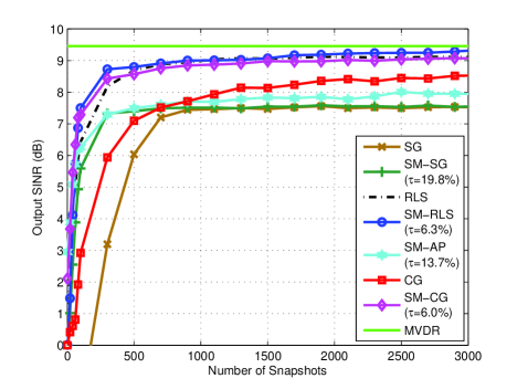
Fig. 2: Output SINR versus the number of snapshots.

The next experiment shows the output SINR performance for the proposed algorithm under a non-stationary scenario, namely, when the number of users changes in the system. The system starts with $q=8$ users including one desired user. The input SNR is $10$ dB and the INR is $35$ dB. The coefficients are the same as those in Fig. 2 except $\alpha=23$. From the first stage (first $3000$ snapshots) of Fig. 3, the proposed algorithm converges quickly to the steady-state. The scenario experiences a sudden change at $N=3000$. We have $4$ more interferers entering the system, which results in the performance degradation for the studied algorithms. The algorithms with the SM technique track this change rapidly and reach the steady-state since the data-selective updates reduce the number of updates and keep a faster convergence rate. Besides, the time-varying bound provides information for them to follow the changes of the scenario. The change also influences the update rate of the algorithms. According to the statistics, the update rate of the proposed algorithm ($\tau=6.2\%$) is rather insensitive to the change and saves computational cost.

Fig. 3: Output SINR versus the number of snapshots in dynamic scenario with additional users enter and/or leave the system.

5 Conclusion

In this paper, we have introduced a new adaptive filtering strategy that combines the SM technique with the adaptive CG algorithm for the LCMV beamformer design. We defined an LCMV optimization problem related to a constraint on the bound of the array output and proposed a CG-based adaptive algorithm for implementation. The proposed algorithm performs the data-selective updates to obtain the filter parameters. For the update, a CG-based vector has been devised to create a relation between the covariance matrix inverse and the steering vector of the desired user. The proposed SM-CG algorithm calculates the CG-based vector to encompass a space of feasible solutions with respect to each time instant and to enforce the constraints. The proposed algorithm exhibits a very good convergence and tracking performance with relatively low computational cost.

References

- [1] O. L. Frost, “An algortihm for linearly constrained adaptive array processing,” IEEE Proc., AP-30, pp. 27-34, 1972.
- [2] S. Haykin, Adaptive Filter Theory, 4rd ed., Englewood Cliffs, NJ: Prentice-Hall, 1996.
- [3] R. C. de Lamare and R. Sampaio-Neto, “Low-Complexity Variable Step-Size Mechanisms for Stochastic Gradient Algorithms in Minimum Variance CDMA Receivers”, IEEE Trans. Signal Processing, vol. 54, pp. 2302 - 2317, June 2006.
- [4] G. D. Mandyam, N. Ahmed, and M. D. Srinath, “Adaptive beamforming based on the conjugate gradient algortihm,” IEEE Trans. Aerospace and Electronics Systems, vol. 33, pp. 343-347, Jan. 1997.
- [5] P. S. Chang and A. N. Willson Jr., “Analysis of conjugate gradient algorithms for adaptive filtering,” IEEE Trans. Signal Processing, vol. 48, pp. 409-418, Feb. 2000.
- [6] N. A. Ahmad, “A globally convergent stochastic pairwise conjugate gradient-based algorithm for adaptive filtering,” IEEE Signal Processing Letters, vol. 15, pp. 914-917, 2008.
- [7] L. Wang and R. C. de Lamare, “Constrained adaptive filtering algorithms based on conjugate gradient techniques for beamforming,” IET Signal Processing, 2010.
- [8] R. C. de Lamare and R. Sampaio-Neto, “Adaptive Reduced-Rank MMSE Filtering with Interpolated FIR Filters and Adaptive Interpolators”, IEEE Sig. Proc. Letters, vol. 12, no. 3, March, 2005.
- [9] R. C. de Lamare, “Adaptive reduced-rank LCMV beamforming algorithms based on joint iterative optimisation of filters,” Electronics Letters, vol. 44, pp. 565-566, Apr. 2008.
- [10] R. C. de Lamare, L. Wang, and R. Fa, “Adaptive reduced-rank LCMV beamforming algorithms based on joint iterative optimization of filters: Design and analysis,” Elsevier Signal Processing, vol. 90, pp. 640-652, Feb. 2010.
- [11] R. C. de Lamare and R. Sampaio-Neto, “Reduced-Rank Adaptive Filtering Based on Joint Iterative Optimization of Adaptive Filters”, IEEE Sig. Proc. Letters, Vol. 14, no. 12, December 2007.
- [12] R. C. de Lamare and R. Sampaio-Neto, “Reduced-Rank Space-Time Adaptive Interference Suppression With Joint Iterative Least Squares Algorithms for Spread-Spectrum Systems,” IEEE Transactions on Vehicular Technology, vol.59, no.3, March 2010, pp.1217-1228.
- [13] R. C. de Lamare and R. Sampaio-Neto, “Adaptive Reduced-Rank Processing Based on Joint and Iterative Interpolation, Decimation, and Filtering,” IEEE Transactions on Signal Processing, vol. 57, no. 7, July 2009, pp. 2503 - 2514.
- [14] R.C. de Lamare, R. Sampaio-Neto, M. Haardt, ”Blind Adaptive Constrained Constant-Modulus Reduced-Rank Interference Suppression Algorithms Based on Interpolation and Switched Decimation,” IEEE Transactions on Signal Processing, vol.59, no.2, pp.681-695, Feb. 2011
- [15] S. Gollamudi, S. Nagaraj, and Y. F. Huang, “Set-membership filtering and a set-membership normalized LMS algorithm with an adaptive step size,” IEEE Signal Processing Letters, vol. 5, pp. 111-114, May 1998.
- [16] S. Nagaraj, S. Gollamudi, S. Kapoor and Y. F. Huang, “BEACON: An adaptive set-membership filtering technique with sparse updates,” IEEE Trans. Signal Processing, vol. 47, pp. 2928-2941, Nov. 1999.
- [17] S. Nagaraj, S. Gollamudi, S. Kapoor and Y. F. Huang, “Adaptive interference suppression for CDMA systems with a worst-case error criterion,” IEEE Trans. Signal Processing, vol. 48, pp. 284-289, Jan. 2000.
- [18] L. Guo and Y. F. Huang, “Frequency-domain set-membership filtering and its applications,” IEEE Trans. Signal Processing, vol. 55, pp. 1326-1338, Apr. 2007.
- [19] R. C. de Lamare and P. S. R. Diniz, “Set-membership adaptive algorithms based on time-varying error bounds for CDMA interference suppression,” IEEE Trans. Vehicular Technology, vol. 58, pp. 644-654, Feb. 2009.
- [20] L. Guo and Y. F. Huang, “Set-membership adaptive filtering with parameter-dependent error bound tuning,” IEEE Proc. Int. Conf. Acoust. Speech and Sig. Proc., 2005.