Directional flow of solitons with asymmetric potential wells: Soliton diode

Abstract

We study the flow of bright solitons through two asymmetric potential wells. The scattering of a soliton by certain type of single potential wells, e.g., Gaussian or Rosen-Morse, is distinguished by a critical velocity above which solitons can transmit almost completely and below which solitons can reflect nearly perfectly. For two such wells in series with certain parameter combinations, we find that there is an appreciable velocity range for which solitons can propagate in one direction only. Our study shows that this directional propagation or diode behavior is due to a combined effect of the sharp transition in the transport coefficients at the critical velocity and a slight reduction in the center-of-mass speed of the soliton while it travels across a potential well.

1 Introduction

The interest in the problem of solitons scattering by external potentials such as barriers [6, 7, 1, 2, 3, 4, 5], wells [8, 9, 10, 11, 12, 13, 14], steps [15, 16, 17], and surfaces [18, 19], stems from the nonlinearity involved and the wave nature of solitons characterizing such process. For instance, the nonlinearity in the Schr$\rm\ddot{o}$dinger equation that controls the evolution of solitons, leads to the nonclassical behavior of partial transmittance and partial reflectance upon scattering a soliton by a potential barrier. The wave nature of solitons results also in a host of other nonclassical scattering outcomes. Of particular importance is the so-called quantum reflection [20]. It has been shown that for slow enough solitons, complete reflection from a potential well [13] or a down potential step takes place [17]. Quantum reflection is caused by a transport of matter or energy from the incident soliton to the bound state of the well which interacts repulsively (attractively) with the original soliton if these are out of phase (in phase). Furthermore, it was found that for a certain type of single potential well, e.g., Gaussian or Rosen-Morse (RM), the two scattering regimes, namely complete quantum reflectance and complete transmittance, are separated by a sharp transition taking place at a critical velocity [13], and this interesting phenomenon has recently been explained for other systems using a delta potential [22, 21].

Another important effect is the reduction in the center-of-mass speed of the soliton as it crosses the potential region. This is due to the fact that transmittance is not complete; a small fraction of the soliton is reflected while most of the soliton is transmitted. The reflected part is typically dispersive and decays in the form of radiation. The larger fraction, i.e., the transmitted part, retains its soliton shape and propagates but with some collective oscillations. The energy for this kind of internal excitation comes from the center-of-mass kinetic energy. As a result, the center-of-mass motion of the soliton slows down.

These two effects, the criticality and the velocity reduction, can be combined in a useful way when two or more RM potentials are placed in series and can lead to novel phenomena. In this letter, we study the dynamics of a soliton in the presence of two RM potential wells with slightly different parameters. One of the interesting effects of this potential combination is the directional flow of solitons. For certain parameter combinations, there is a velocity window for which solitons can propagate freely with nearly full transmission in one direction and blocked with almost perfect reflection in the other direction. We termed this behavior as “soliton diode”. Asymmetric electron flow with two tunneling barriers was studied [23, 24, 26, 25] and for solitons this behavior has recently been demonstrated for a discrete nonlinear Schr$\rm\ddot{o}$dinger equation with asymmetric potentials [27]. While we obtain the transport coefficients for the soliton diode numerically by solving the appropriate Gross-Pitaevskii (GP) equation, we support our qualitative explanation of this effect by investigating in detail the dependence of the critical velocity and the velocity reduction for each potential well separately in terms of the parameters of the wells and the speed of the incident soliton. This allowed for an independent and accurate account of the velocity window for which this diode functions.

2 Theoretical Model

In the presence of an external potential $V(x)$ the dynamics of bright soliton is governed by the one-dimensional GP equation, which can be written in standard dimensionless (for explicit units, see, for example, Ref. [28]) form as

$$i{\partial\over\partial t}\psi(x,t)=\left[-{1\over 2}{\partial^{2}\over\partial x^{2}}+V(x)+g|\psi(x,t)|^{2}\right]\,\psi(x,t),$$ (1)

where we choose the potential $V(x)$ of the form

$$V(x)=-{V_{1}}\,{{\rm sech}^{2}\left[\alpha_{1}(x-x_{\rm cm1})\right]}-{V_{2}}\,{{\rm sech}^{2}\left[\alpha_{2}(x-x_{\rm cm2})\right]}.$$ (2)

Here, $V_{1,2}$, $\alpha_{1,2}$, and $x_{\rm cm1,2}$ determine the depth, inverse width, and the position of the center of the first and second potential wells, respectively. This potential, which is known in the literature as the Rosen-Morse potential, belongs to the class of reflectionless potentials which may transmit without reflection in the linear regime. The factor $g$ denotes the mean-field interaction strength and we take $g=-1$. In our numerical simulation we prepare an initial state far away from the potential region and propagate it in real time. We always choose our initial wave function as the exact solution of the homogeneous version of Eq. (1), namely

$$\psi(x,t=0)={A}\,e^{i\,v(x-x_{\rm cm})}{{\rm sech}\left[A(x-x_{\rm cm})\right]},$$ (3)

with $A=1$ and $x_{\rm cm}=x_{0}+v\,t$, where $v$ and $x_{0}$ are the initial center-of-mass velocity and position, respectively. The evolution time is taken long enough for the scattered soliton to be far away from the potential. Then, we calculate the reflection, trapping, and transmission coefficients. For the left-to-right moving soliton with a single potential well, we define the reflection, trapping, and the transmission coefficients as: $R=(1/N)\,\int_{-\infty}^{-l}|\psi(x,t)|^{2}\,dx$, $L=(1/N)\,\int_{-l}^{l}|\psi(x,t)|^{2}\,dx$, and $T=(1/N)\,\int_{l}^{\infty}|\psi(x,t)|^{2}\,dx$, where $l\approx 5/\alpha$ from the center of the well and $N$ is the normalization of the soliton given by $N=\int_{-\infty}^{\infty}|\psi(x,t)|^{2}\,dx$. For right-to-left moving soliton, $R$ and $T$ are interchanged but $L$ remains the same. For the present case of two potential wells in series, we take $-l$ to be on the left of the left well and $l$ to be on the right of the right well.

3 Results: The Diode Behavior

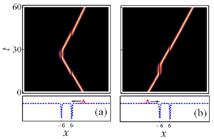
Figure 2: (Color online) Figures (a) and (b) show the spatio-temporal density plots with schematics for a case with $|v|=0.33$, which corresponds to the dots in Figs. 1(a) and (b), respectively. The parameter set is same as in Fig. 1

We present the main findings of our study here. We consider two RM potential wells in series with slightly different parameters (See the schematic figures in Figs. 2(a) and (b) below.). For this set of potential wells, the soliton is reflected for small enough velocity and transmitted for large velocity. The transition from high reflection to high transmission is very sharp. Figures 1 (a) and (b) show the reflectance $R$ and transmittance $T$ versus the magnitude of the incident soliton velocity $v$ for the potential given by (2) with $V_{1}=4.35$, $V_{2}=4.0$, $\alpha_{1}=\alpha_{2}=2$, and $x_{\rm cm1}=-x_{\rm cm2}=6$. Solid and dashed lines in Fig. 1(a) show the reflection coefficient for the right-to-left moving and left-to-right soliton, respectively. Figure 1(b) shows the transmittance for both cases. For the left-moving soliton there is a critical velocity for which there is a sudden jump from mostly reflectance to mostly transmittance. Similar behavior exists for the right-moving soliton with another critical velocity. Surprisingly, there is a difference in between the two critical velocities for the left- and right-moving solitons. As a result, there is a small but appreciable velocity window for which there is almost full transmittance in one direction and nearly zero transmittance in the other direction, i.e., the soliton shows directional propagation for this set of parameters. This behavior is similar to the diode effect in semiconductor physics. Figures 2(a) and (b) show the spatio-temporal plots corresponding to a selected value of the initial speed. Figure 2(a) corresponds to a soliton incident from the right of the right well with incident velocity $v=-0.33$. The soliton is first transmitted through the right well (centered at $6$) and then reflected to the right by the left well (centered at $-6$) and finally transmitted to the right through the right well. The overall reflection coefficient is $R\approx 0.98$ and is marked by a filled circle in Fig. 1(a). Figure 2(b) corresponds to a soliton incident from the left of the left well and propagates to the right with the same magnitude of the incident velocity $v=0.33$. This time the soliton is transmitted through both wells. The overall transmission coefficient is $T\approx 0.99$ and is also marked by a filled circle in Fig. 1(b).

This novel diode behavior of soliton propagation can simply be explained by a combined effect of the critical velocity and the reduction in the soliton’s center-of-mass speed caused by a potential well. Consider a soliton injected on a single potential well with a speed slightly larger than the critical velocity. The flow is naturally symmetric with full transmission from both sides. Introducing another potential well with considerably lower critical velocity, say to the right of the first one, breaks this symmetry. While the soliton incident from the left transmits both the wells, the soliton from the right with the same incident speed can only transmit the well on the right since, as it crosses that well, it suffers a velocity reduction which is small but enough to reduce the soliton’s speed to below the critical velocity of the left well. Therefore, the soliton will be reflected from the left well to the right. Since the critical velocity of the right well is still considerably lower than the speed of the reflected soliton, the soliton will continue its motion in the right direction. In this manner, both the initially left-moving and the right-moving solitons end up moving to the right.

As a specific example, we calculate, for the potential wells considered in Figs. 2(a) and (b), the critical velocities of the left and right wells, $v_{cr}^{l}$ and $v_{cr}^{r}$, respectively, which take the values: $v_{cr}^{l}=0.3275$ and $v_{cr}^{r}=0.1175$. Let us consider the case of the soliton with incident velocity $v=0.33$. For this incident velocity, the velocity reductions are $\Delta v^{l}=0.015$ and $\Delta v^{r}=0.014$. If it is incident from the left, it will transmit through the left well as the velocity is larger than $v_{cr}^{l}$. The transmitted soliton will have the reduced velocity $v=0.315$ which is still larger than $v_{cr}^{r}$, allowing the soliton to transmit through the right well to the right. Now if the soliton is incident from the right side of the right well, it will transmit through it, as the soliton’s velocity $v=0.33$ is larger than $v_{cr}^{r}$. Due to the velocity reduction by the right well, the soliton’s velocity reduces to $v=0.316$ which is less than the $v_{cr}^{l}$, and therefore, the soliton will be reflected by the left well to the right. Finally it will be transmitted through the right well to the right. So whether the soliton is incident from the right or from the left, it will always end up moving to the right and there is no flow in the left direction for the velocity considered.

Having demonstrated the function of the diode for a specific set of the system’s parameters and a single soliton’s initial speed, a thorough investigation of this phenomenon in terms of these parameters is in order. Specifically, we want to account for the velocity window in Fig. 1 over which the diode functions. In addition, we want to find the effect of the potentials’ parameters on the width of this window with the aim of finding the optimized potentials’ parameters that lead to the maximum velocity window.

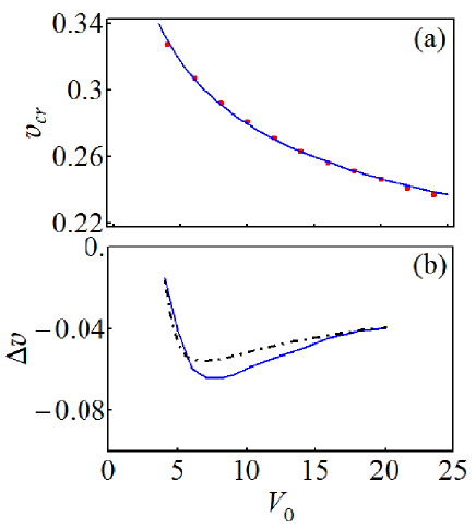
Figure 3: (Color Online) (a) Critical velocity $v_{cr}$ as a function of the well depth $V_{0}$ of the RM potential with $\alpha=\sqrt{V_{0}}$. (b) Solid curve shows the velocity shift as a function of the well depth $V_{0}$ of the RM potential with $\alpha=\sqrt{V_{0}}$ for fixed incident velocity $v=0.33$. Dash-dotted curve shows the velocity shift as a function of the well depth derived semi analytically.

We start by characterizing the effect of a single potential well, $V(x)=-{V_{0}}\,{{\rm sech}^{2}(\alpha\,x)}$, on the propagation of solitons. We found that it is essential to set $\alpha=\sqrt{V_{0}}$ in order to get a sharp transition of the transport coefficients at the critical velocity. For such particular type of potential well, the width of the well decreases with increasing the well depth. The critical velocity turns out to be a monotonic decreasing function of the well depth. Figure 3(a) shows the critical velocity, defined by $v_{cr}=(v_{1}+v_{2})/2$ as a function of the well depth $V_{0}$. Here $v_{1}$ is the largest velocity with almost full reflection and $v_{2}$ is the smallest velocity with nearly perfect transmission. Circles show our numerical data and the solid line shows the fit of the data by $v_{cr}\approx 0.42\,V_{0}^{-0.18}$. Currently we are unable to find a convincing explanation to this trend.

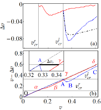
Figure 4: (Color Online) (a) The velocity shift as a function of the incident velocity. Solid curve shows the velocity shift for $V_{0}=4.35$ and $\alpha=2$ and dashed curve shows that for $V_{0}=4$ and $\alpha=2$. Dash-dotted curve shows the velocity shift as a function of the incident velocity derived semi analytically for $V_{0}=4$. The vertical lines show the critical velocities for the two well depths. (b) Reduced velocity versus incident velocity. The horizontal lines show the critical velocities for the two well depths. The solid and dashed curves show the reduced velocity for the left and the right moving solitons, respectively. The inset shows, with the thick horizontal line, the velocity range for which the diode functions.

Besides the critical velocity, it is also essential to calculate the velocity reduction in terms of the system’s parameters. The velocity shift $\Delta v$ is defined as the difference between the incident velocity and the velocity of the scattered soliton well after crossing the potential region. This depends on the depth and width of the potential well as well as on the magnitude of the incident velocity. Figure 3(b) shows the shift in velocity as a function of the well depth $V_{0}$ for fixed incident velocity $v=0.33$. This velocity is slightly larger than the critical velocity $v_{cr}=0.3275$ for $V_{0}=4$ and $\alpha=2$. The shift in velocity also depends on the magnitude of the incident velocity. The solid and dashed curves in Fig. 4(a) show the shift in velocity for incident velocities greater than the critical velocity $v_{cr}$ and for fixed well depths $V_{0}=4.35$ and $V_{0}=4$, respectively, with $\alpha=2$. We calculate the velocity shift by monitoring the position of the density maxima as function of the evolution time. The slope of this curve gives the velocity and we calculate two velocities one before the interaction with the potential well and one after the interaction with the well. Both are measured far from the interaction region.

To understand the physics of the diode’s function, we employ a variational calculation that confirms our previous arguments based on the numerical results and specifically accounts for the velocity reduction shown in Figs. 3 (b) and 4 (a). Following Refs. [9, 13], we use an ansatz function that takes into account the incident soliton and a trapped mode, namely $\Psi(x,t)=\psi_{1}(x,t)+\psi_{2}(x,t)$, where $\psi_{1}(x,t)=A_{1}\,{\rm sech}[A_{1}\,(x-\eta_{1})]\,{\rm exp}[i\phi_{1}+iv_{1}x]$ and $\psi_{2}(x,t)=A_{2}\,{\rm sech}[x/q_{1}]\,{\rm exp}[i\phi_{2}+i\,\sigma_{2}\,{\rm log\,cosh}(x/q_{2})]$. Here $A_{1}$, $v_{1}$, $\eta_{1}$, and $\phi_{1}$ denote the amplitude, velocity, center of mass position, and the phase of the incoming soliton and $A_{2}$, $q_{2}$, $\sigma_{2}$, and $\phi_{2}$ denote the amplitude, width, chirp parameter, and the phase of the trapped mode, respectively. For simplicity, the potential is approximated by the delta function $V(x)=-V_{0}\delta(x)$. After constructing the Lagrangian, $L=\int_{\infty}^{\infty}dx\left[\frac{i}{2}(\Psi^{*}\frac{\partial}{\partial t}\Psi-\Psi\frac{\partial}{\partial t}\Psi^{*})-\frac{1}{2}|\frac{\partial}{\partial x}\Psi|^{2}+\frac{1}{2}|\Psi|^{4}+V|\Psi|^{2}\right]$, we derive the Euler-Lagrange equations for the variational parameters. From the set of resulting equations, we derive the following equation for the center of mass position of the soliton

$$\ddot{\eta_{1}} = \dot{v_{1}}-\frac{d}{dt}\left(\frac{\dot{A_{1}}}{A_{1}}\right)\eta_{1}-\left(\frac{\dot{A_{1}}}{A_{1}}\right)\dot{\eta_{1}},$$ (4)

where $\dot{A_{1}}/A_{1}=V_{0}\,A_{2}\,{\rm sech}(A_{1}\,\eta_{1})\sin(\Delta\phi)$ and $\dot{v_{1}}=-V_{0}\,A_{1}\,{\rm sech}(A_{1}\,\eta_{1})\tanh(A_{1}\,\eta_{1})\left[A_{2}\cos(\Delta\phi)+A_{1}\,{\rm sech}(A_{1}\,\eta_{1})\right]$ with $\Delta\phi=\phi_{1}-\phi_{2}$ and $\dot{}$ denotes the time derivative. From this equation it is clear that the potential well plays the role of a damping factor with a damping coefficient $-{\dot{A}_{1}}/A_{1}$. Assuming $2\beta$ be the effective distance over which the soliton experiences such a frictional force, the velocity reduction can be shown to take the form

$$\Delta v\approx-2V_{0}\beta A_{1}A_{2}{\rm sech}(A_{1}\,\eta_{1})\sin(\Delta\phi),$$ (5)

which is proportional to the trapped mode amplitude $A_{2}$. If the transmission is perfect, i.e., $A_{1}=1$ and $A_{2}=0$, there is no velocity reduction. From this simple argument it is obvious that the reduction in velocity arises primarily due to the imperfect transmission after the critical velocity. In Fig. 1(b), the transmission coefficient curve acquires a slight downward curvature. It is this particular behavior that mainly accounts for the velocity reduction. Specifically, the coefficient of the trapped mode $A_{2}$ is proportional to $1-T$. To verify this, we have calculated $A_{1}$ and $A_{2}$ numerically in terms of the incident velocity and the well depth. In addition, we approximated $\Delta\phi$ by its value near the trap center, namely $-.21\pi$ (See Fig. 7 in Ref. [14]), and set $\eta=0$. Finally, we set $V_{0}\beta=1/\sqrt{2\pi}$, which is a good approximation for delta potentials. As a result, we obtain the velocity reduction as a function of the well depth and the incident velocity plotted with dashed-dotted curves in Fig. 3(b) and Fig. 4(a), respectively, which able to capture the main features qualitatively.

The mechanism by which the diode functions, can now be explained in Figure 4(b). The solid and dashed curves show the reduced velocity of the soliton after crossing a single potential well for the two cases of $V_{0}=4.35$ and $V_{0}=4$ with $\alpha=2$. The dotted diagonal line shows the velocity of the incident soliton. The two horizontal lines mark the critical velocities of the two wells. For the left-to-right-moving soliton we follow the dashed curve marked as $OABC$. For $OA$, where the point $A$ corresponds to $v=v_{cr}^{l}$, the incident velocity is smaller than the critical velocity $v_{cr}^{l}=0.3275$ of the left well and the soliton is reflected back to the left. For $v>v_{cr}^{l}$ we follow the curve $ABC$, where the reduced velocity is well above the critical velocity $v_{cr}^{r}=0.1175$ of the right well and the soliton is transmitted to the right. Therefore, from left to right, the soliton is reflected for $v<v_{cr}^{l}$ and transmitted for $v>v_{cr}^{l}$. On the other hand, for the right-to-left-moving soliton we follow the solid curve marked as $O\alpha\beta\gamma\delta$. For $O\alpha$, the incident velocity is smaller than the critical velocity $v_{cr}^{r}$ of the right well and the soliton is reflected back to the right. For $v>v_{cr}^{r}$ we follow the line $\alpha\beta\gamma$, where the point $\gamma$ corresponds to $v_{cr}^{l}+|\Delta v^{r}|$. Here, the reduced velocity is well above the critical velocity $v_{cr}^{r}$ of the right well but smaller than the critical velocity $v_{cr}^{l}$ of the left well. As a result the soliton is reflected by the left well and transmitted to the right through the right well. For $\gamma\delta$ the reduced velocity is greater than the critical velocity $v_{cr}^{l}$ of the left well and the soliton is transmitted to the left. In conclusion, the right-moving soliton will transmit to the right for $v>v_{cr}^{l}$ and the left-moving soliton will reflect to the right for $v<v_{cr}^{l}+|\Delta v^{r}|$. As a result, the scattered soliton will always be flowing to the right irrespective of the direction of the incoming soliton provided its incident speed is in the velocity range $v_{cr}^{l}<v<v_{cr}^{l}+|\Delta v^{r}|$. The width of this velocity window $|\Delta v^{r}|\approx 0.01$ agrees well with that obtained directly from the numerical solution of the GP equation, as can be seen by comparing Fig. 1(a) and the inset of Fig. 4(b). It is essential to note that the velocity reduction should be considerably larger than the velocity range over which the transition at the critical velocity takes place. If this condition is not met then partial transmission and reflection, with comparable magnitudes, takes place resulting in a failure of the function of the diode.

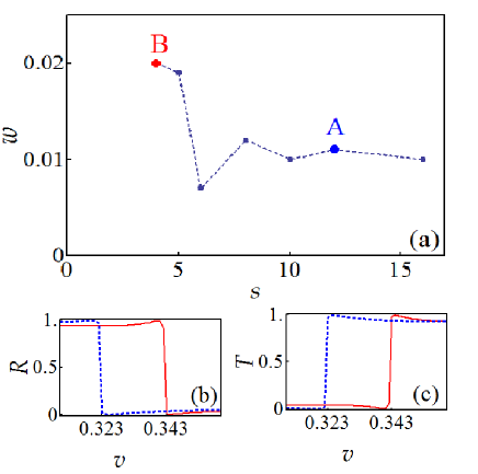
Figure 5: (Color online) (a) Velocity window $w$ as a function of the separation $s$ between the centers of the wells. The width and depth of the wells are fixed. Dashed line is drawn to guide the eye. The points marked as $A$ and $B$ are the separations which are used for Fig. 1 and Figs. 4 (b) and (c), respectively. (b) Solid and dashed lines show the reflection coefficients for the left and the right moving solitons, respectively. (c) Solid and dashed lines show the transmission coefficients for the left and the right moving solitons, respectively. Position of the well centers are $x_{\rm cm1}=-x_{\rm cm2}=2$. All the other parameters are same as in Fig. 1

When the two wells are well separated, the effect of the either of them is independent of the other. As we move the wells closer, they couple together after a certain small separation and start to affect the soliton propagation in a combined manner. Due to this coupling between the wells and nonlinearity of the soliton dynamics, there is a non-monotonous change in the velocity window for which the diode effect is observed. Figure 5(a) shows the width of the velocity window $w$ as function of the separation $s$ between the wells. We define the window width $w$ as the difference between the critical velocities of the solitons transmitting from opposite directions. The separation $s$ is the distance between the centers of the two wells. Figures 5(b) and (c) show the reflectance and transmittance as a function of the incident velocity of the soliton. Note that velocity window is now almost doubled compared to that shown in Figs. 1(a) and (b).

The directional flow of soliton with asymmetric potential wells can also be achieved with two Gaussian wells with appropriate parameter combination. Gaussian potential supports both criticality [13] and velocity reduction for soliton propagation. For example, the potential $V(x)=-4.35\exp[{-3(x-6)^{2}}]-4.0\exp[{-3(x+6)^{2}}]$ shows diode behavior in the range $0.304\leq v\leq 0.310$. Therefore, the directional flow is not unique to a series of RM potentials.

The combined effect of the velocity reduction and criticality can also be used to trap solitons. If the reduction in velocity changes the velocity such that it is smaller than any of the two critical velocities then the soliton will be trapped in between the potential wells and oscillates. One such parameters combination is $v=0.33$, $V_{1}=V_{2}=4$, $\alpha_{1}=\alpha_{2}=2$, and $x_{\rm cm1}=-x_{\rm cm2}=6$. For this set of parameters, if the soliton is incident from left or from right it can transmit through the first well and the reduced velocity becomes $v=0.315$, which is smaller than $v_{cr}^{l}=v_{cr}^{r}=0.3275$ and oscillates between the two wells.

For multiple soliton cases, we find similar behaviors as for single soliton case only if the initial soliton separation is very large compared to soliton width. In this regard, we use a chain of two solitons, which are initially located at, say, $x_{\rm cm}=20$ and $x_{\rm cm}=60$. Qualitatively we get the same diode behavior as shown in Fig. 1. For smaller initial separation, the nonlinearity and the interaction near the potential regions destroy the diode effect.

4 Discussion and Conclusions

Our numerical study of the dynamics of one-dimensional GP equation with two asymmetric potential wells (Gaussian or Rosen-Morse) shows that the soliton can propagate in one direction for a certain velocity range and with certain parameter combinations. This unidirectional propagation arises due to the criticality and the velocity reduction by a single potential well. When two such potentials with slightly different parameters are in series, the combined effect causes the soliton to move in one direction only. A detailed account of the critical velocities and velocity reductions of both potential wells explains this effect and predicts the velocity range over which the diode functions, in a good agreement with the numerical result. We also employ a variational calculation and estimate the velocity reduction as a function of the input velocity and the depth of the potential well. The semi analytical velocity reduction curves able to capture the main feature of the corresponding exact numerical ones qualitatively.

The function of the soliton diode was demonstrated here for a single pair of potential depths $V_{1}=4.35$ and $V_{2}=4.0$. The width of the velocity window for which the diode works properly, certainly depends on the values and ratio of these two parameters as well as on the widths of the potential wells and their separation. Thus, widening the velocity window and increasing the diode’s efficiency requires further systematic investigation of the effect of these parameters as well investigating other types of potential wells.

The GP equation considered here is the governing equation of the dynamics of both matter-wave solitons in Bose-Einstein condensates [29, 30] and optical solitons in optical fibers. Therefore, it is expected that the diode behavior found here to be realized in both cases. For the case of optical solitons, this diode may be a favorable instrument in achieving all-optical communication and computation in optical fibers.

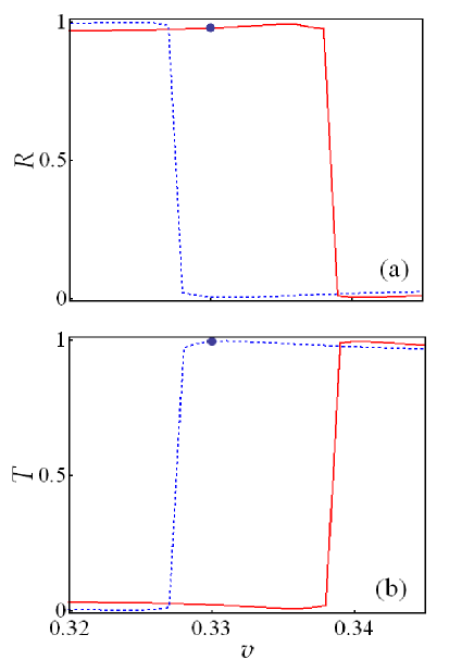
Figure 1: (Color online) (a) Solid and dashed lines show the reflection coefficients for the left and the right moving soliton, respectively. (b) Solid and dashed lines show the transmission coefficients for the left and the right moving soliton, respectively. The parameter set is as follows: $V_{1}=4.35$, $V_{2}=4.0$, $\alpha_{1}=\alpha_{2}=2$, and $x_{\rm cm1}=-x_{\rm cm2}=6$.

- [1] K. Forinash, M. Peyrard, and B. Malomed, Phys. Rev. E 49, 3400 (1994).
- [2] X. Cao and B. Malomed, Phys. Lett. A 206, 177 (1995).
- [3] D. J. Frantzeskakis, G. Theocharis, F. K. Diakonos, P. Schmelcher, and Y. S. Kivshar, Phys. Rev. A 66, 053608 (2002).
- [4] A. E. Miroshnichenko, S. Flach, and B. Malomed, Chaos 13, 874 (2003).
- [5] V. Ahufinger, A. Mebrahtu, R. Corbal an, and A. Sanpera, New J. Phys. 9, 4 (2007).
- [6] C. Weiss and Y. Castin, Phys. Rev. Lett. 102, 010403 (2009).
- [7] A. I. Streltsov, O. E. Alon, and L. S. Cederbaum, J. Phys. B 42, 091004 (2009); Phys. Rev. A 80, 043616 (2009).
- [8] Y. S. Kivshar, Z. Fei, and L. Vzquez, Phys. Rev. Lett. 67, 1177 (1991).
- [9] R. H. Goodman, P. J. Holmes, and M. I. Weinstein, Physica D 192, 215 (2004).
- [10] H. Sakaguchi and M. Tamura, J. Phys. Soc. Jpn. 73, 503 (2004).
- [11] K. T. Stoychev, M. T. Primatarowa, and R. S. Kamburova, Phys. Rev. E 70, 066622 (2004).
- [12] L. Morales-Molina and R. A. Vicencio, Opt. Lett. 31, 966 (2006).
- [13] C. Lee and J. Brand, Europhys. Lett. 73, 321 (2006).
- [14] T. Ernst and J. Brand, Phys. Rev. A 81, 033614 (2010).
- [15] A. B. Aceves, J. V. Moloney, and A. C. Newell, Phys. Rev. A 39, 1809 (1989).
- [16] Y. S. Kivshar, A. M. Kosevich, and O. A. Chubykalo, Phys. Rev. A 41, 1677 (1990).
- [17] S. Cornish, N. Parker, A.Martin, T. Judd, R. Scott, T. Fromhold, and C. Adams, Physica D 238, 1299 (2009).
- [18] T. A. Pasquini, Y. Shin, C. Sanner, M. Saba, A. Schirotzek, D. E. Pritchard, and W. Ketterle, Phys. Rev. Lett. 93, 223201 (2004).
- [19] T. A. Pasquini, M. Saba, G.-B. Jo, Y. Shin, W. Ketterle, D. E. Pritchard, T. A. Savas, and N. Mulders, Phys. Rev. Lett. 97, 093201 (2006).
- [20] H. Friedrich and J. Trost, Phys. Rep. 397, 359 (2004).
- [21] C-H. Wang, T-M. Hong, R-K. Lee, and D-W. Wang, Optics Express 20, 22675 (2012).
- [22] B. Gertjerenken, T. P. Billam, L. Khaykovich, and C. Weiss, Phys. Rev. A 86, 033608 (2012).
- [23] J. Chen, J. G. Chen, C. H. Yang, and R. A. Wilson, J. Appl. Phys. 70(6), 3131 (1991).
- [24] M. Tewordt, L. Martn-Moreno, J. T. Nicholls, M. Pepper, M. J. Kelly, V. J. Law, D. A. Ritchie, J. E. F. Frost, and G. A. C. Jones, Phys. Rev. B 45, 14407 (1992).
- [25] H. B. de Carvalho, M. J. S. P. Brasil, V. Lopez-Richard, Y. Galvo Gobato, G. E. Marques, I. Camps, L. C. O. Dacal, M. Henini, L. Eaves, and G. Hill, Phys. Rev. B 74, 041305(R) (2006).
- [26] M. Chshiev, D. Stoeffler, A. Vedyayev, and K. Ounadjela, Europhys. Lett. 58 257 (2002).
- [27] S. Lepri and G. Casati, Phys. Rev. Lett. 106, 164101 (2011).
- [28] L. F. Mollenauer and J. P. Gordon, Solitons in Optical Fibers: Fundamentals and Applications (Academic Press) 2006.
- [29] K. E. Strecker, G. B. Partridge, A. G. Truscott, and R. G. Hulet, Nature 417, 150 (2002).
- [30] L. Khaykovich, F. Schreck, G. Ferrari, T. Bourdel, J. Cubizolles, L. D. Carr, Y. Castin, and C. Salomon, Science 296, 5571 (2002).