Spectral Theory for Networks with Attractive and Repulsive Interactions

Abstract

There is a wealth of applied problems that can be posed as a dynamical system defined on a network with both attractive and repulsive interactions. Some examples include: understanding synchronization properties of nonlinear oscillator;, the behavior of groups, or cliques, in social networks; the study of optimal convergence for consensus algorithm; and many other examples. Frequently the problems involve computing the index of a matrix, i.e. the number of positive and negative eigenvalues, and the dimension of the kernel. In this paper we consider one of the most common examples, where the matrix takes the form of a signed graph Laplacian. We show that the there are topological constraints on the index of the Laplacian matrix related to the dimension of a certain homology group. In certain situations, when the homology group is trivial, the index of the operator is rigid and is determined only by the topology of the network and is independent of the strengths of the interactions. In general these constraints give upper and lower bounds on the number of positive and negative eigenvalues, with the dimension of the homology group counting the number of eigenvalue crossings. The homology group also gives a natural decomposition of the dynamics into “fixed” degrees of freedom, whose index does not depend on the edge-weights, and an orthogonal set of “free” degrees of freedom, whose index changes as the edge weights change. We also present some numerical studies of this problem for large random matrices.

1 Introduction

1.1 Problem Formulation

There are many applied problems that can ultimately be reduced to the question of understanding a dynamical problem on a network or graph. In these applications it is often important to understand the dynamical behavior of the evolution in terms of the topological properties of the graph.

In this paper we consider a simple, connected, undirected edge-weighted graph ${\Gamma}=(V({\Gamma}),E({\Gamma}))$ with vertex set $V(\Gamma)$ and edge set $E(\Gamma)$. For each edge in $E(\Gamma)$ connecting vertex $i$ with vertex $j$ we associate a weight $\gamma_{ij},$ which is assumed to be non-zero but may take either sign. If there is no edge connecting vertices $i$ and $j$ the weight $\gamma_{ij}$ is understood to be zero.

For such a graph we define the signed Laplacian matrix $\mathcal{L}({\Gamma})$ by

$$\mathcal{L}({\Gamma})_{ij}=\begin{cases}\gamma_{ij},&i\neq j,\\ -\sum_{k\neq i}\gamma_{ik},&i=j.\end{cases}$$ (1.1)

Note that $\mathcal{L}({\Gamma})$ is symmetric, so all eigenvalues of $\mathcal{L}({\Gamma})$ are real. If the weights are all positive, $\gamma_{ij}>0,$ this is a standard graph Laplacian and as such the spectrum of ${\mathcal{L}}$ is well-understood: $\mathcal{L}$ is a negative semi-definite matrix, with the dimension of the kernel equal to the number of connected components of the graph ${\Gamma}$. In many applications the weights are not guaranteed to be positive. In this case the matrix is no longer definite, and we are interested in determining the number of positive, zero, and negative eigenvalues of $\mathcal{L}({\Gamma})$, which we denote as $n_{+}({\Gamma}),n_{0}({\Gamma}),n_{-}({\Gamma})$ respectively.

In particular, we would like to determine topological bounds on these indices, i.e. conditions that depend only on the arrangement of signs of the edge weights $\gamma_{ij}$, and not on their magnitudes. We are aware of at least five applied problems that motivate this question:

1. Stability of Fixed Points Consider any dynamical system defined on the network. Specifically given a graph ${\Gamma}$, and symmetric coupling functions $\varphi_{ij}(\cdot)=\varphi_{ji}(\cdot)$ associated to edges in the graph we define a dynamical system as follows

   $$\frac{d}{dt}x_{i}=F_{i}({\mathbf{x}}):=\omega_{i}+\sum_{j\in{\Gamma}}\varphi_{ij}(x_{j}-x_{i}).$$ (1.2)

   A well-studied example of this type of dynamical system is the Kuramoto oscillator [38, 29, 30, 40, 2], where we choose $\varphi_{ij}(\cdot)=\gamma_{ij}\sin(\cdot)$.

   To compute the stability index of a fixed point for the system (1.2), i.e. a vector $\mathbf{x}$ with $F_{i}(\mathbf{x})=0$ for all $i$, we need to determine the index of the Jacobian $J$, where

   $$J_{ij}=\begin{cases}\varphi_{ij}^{\prime}(x_{j}-x_{i}),&i\neq j,\\ -\sum_{k}\varphi_{ik}^{\prime}(x_{k}-x_{i}),&i=j.\end{cases}$$

   The Jacobian $J$ is a graph Laplacian of the form (1.1); thus, determining the stability indices for fixed points of (1.2) is equivalent to the problem studied here [32, 42, 43, 33, 31, 4]. When studying this dynamical system, the first object of study is always the stable points. But, for example, if we consider such a system perturbed by a small stochastic process, then gaining a qualitative understanding of the dynamics requires that we identify all of the 1-saddles, i.e. those points which are unstable but with exactly one unstable direction (e.g. see [11]).

   The $\varphi^{\prime}_{ij}$ terms in $J$ can be of either sign, making it natural to consider the case of a graph Laplacian with arbitrary signs on the weights. For a generic choice of coupling functions, $\varphi^{\prime}_{ij}(x_{i}-x_{j})$ is non-zero for all $i,j$, implying that the graph determining $J$ and the graph defined by the original interactions in (1.2) have the same underlying topology.

2. Stability of Neural Networks If we consider any neural network system with both “positive” and “negative feedbacks”, then the stability analysis reduces to a eigenvalue problem similar to  (1.1). In biological applications the interaction strengths are both difficult to measure experimentally and (due to neural plasticity) very changeable. This makes it impractical to estimate the magnitudes of $\gamma_{ij}$ with any degree of reliability. On the other hand the nature of the interaction (excitatory or inhibitory) is anatomical and, in general, will not change. Thus we have reliable experimental data on the signs of various connections, but very little reliable information on the magnitudes. This makes the idea of understanding the extent to which the dynamics is determined by the topology of the network a very attractive one.

3. Convergence of Consensus Algorithms It was pointed out by Xiao and Boyd [44] that for some graphs, the optimal choice of weights for the convergence of a consensus algorithm uses negative weights. In particular, given a weighted graph ${\Gamma}=\{\gamma_{ij}\}$, define the linear discrete-time consensus algorithm given by

   $$x_{i}(t+1):=\sum_{j}\gamma_{ij}x_{j}(t).$$ (1.3)

   The question posed in [44] is how one might optimize the choice of $\gamma_{ij}$, given the underlying graph topology and the constraint that $\mathbf{1}$ be a stable fixed point of (1.3), to obtain the most rapid convergence to consensus (to wit, to make the Lyapunov exponent of (1.3) as small as possible). It was observed there that there exist examples of graphs where the optimal choice involves negative weights—that is to say, that there are choices of weights that make (1.3) converge more rapidly than the most rapidly-mixing Markov chain. This observation inspired a deluge of work (examples include [17, 35, 22, 45]) on this fast convergence problem and it has been observed that the need for negative weights is typical in many contexts.

   Of course, one obvious constraint on determining the optimal choice of weights is that $n_{+}({\Gamma})=0$ so that we obtain convergence at all. In the work mentioned above, this was always obtained by solving a semidefinite programming problem over the set of all weights associated to a particular unweighted graph ${\Gamma}$. The results in the current work give topological (i.e. weight-independent) bounds for $n_{+}({\Gamma})$.

4. Clustering in Social Networks Questions of this sort arise in the study of social networks. In the classic work of Hage and Harary [16], matrices of the form (1.1) modeled the interaction of tribal groups within an alliance in New Guinea. In this work the underlying graph has sixteen vertices, representing the different tribal units, with edges represent relations between different tribal groups. These relations can be friendly (“rova”) or antagonistic (“hina”) corresponding to $\gamma_{ij}>0$ and $\gamma_{ij}<0$ respectively. Another anthropological example is the SlashDot Zoo, a social network associated to the website SlashDot [1]. On this website participants can label each other as friend or foe. In the context of social network models the index $n_{+}({\Gamma})$ indicates the tendency of the network to separate into mutually antagonistic subgroups.

5. Resistor Networks with Negative Resistance One intuitively appealing way to think about a signed graph Laplacian is as a network of resistors where some of the edges have negative resistance. While perfect negative resistors cannot be implemented with passive components there are many nonlinear components whose current-voltage curves are non-monotone, and have a region where the current is a decreasing function of the voltage. In the region where the current is a decreasing function of current the component has negative (differential) resistance. Some examples of such components include tunnel and Gunn diodes, neon lamps, and certain kinds of tubes. Circuits built from these components often exhibit multi-stability, and the stability of a given solution is governed by a system of the form (1.1). Alternatively a negative resistance can be implemented using active circuit elements with gain, such as an operational amplifier (op-amp).

On a somewhat different note we should remark that signed graphs and signed Laplacians arise very naturally in knot theory. One classical result of this kind is a procedure for associating a quadratic form to a knot originally due to Goeritz [13, 14]. In Goeritz’s construction one considers a planar projection of the knot, with regions of plane alternately colored black and white. Two regions of given color are connected by an edge if they share a crossing. The weight attached to the edge is $+1$ if the crossing is left-handed and $-1$ if the crossing is right-handed. The reduced determinant — the product over the non-zero eigenvalues of the associated graph Laplacian — can be shown to be a knot invariant. Related results include a construction by Kauffman of a Tutte polynomial for signed graphs [25] which specializes to known invariants like the Jones [21] and Kauffman bracket polynomials [24]. This construction was further generalized to matroids by Zaslavsky [49]. Signed graphs and their Laplacians have also been studied in the graph theory community independent of their connection to knot theory (see [48, 47, 46] and following, also [18]) but the the reader should be aware that there are several different generalizations of the Laplacian to the case where negatively weighted edges are allowed. In one variation definition the diagonal entries are taken to be minus the sum of the absolute values of the edge weights. In this case the matrix is typically not zero-sum, and is negative semi-definite. Clearly the spectral questions are different and there is no obvious correspondence between the two.

To make clear the kinds of questions we want to ask, and the kind of phenomena we would like to understand, we begin with an example of two networks.

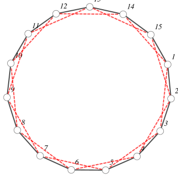
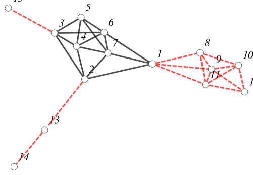
Figure 1: Two graphs on 15 nodes. Here we are represented positively weighted edges with solid black lines, and negatively weighted edges by dashed red lines.

Example 1.1

Figure 1 depicts two signed graphs representing networks. in this figure dashed lines (red online) represent negative/excitatory/hina interactions and the solid line represent positive/inhibitory/rova interactions. Each of these graphs has fifteen vertices, fifteen hina edges and fifteen rova edges. The dynamics, however, are typically very different. We claim that there is a marked difference between the way mathematicians tend to view these problems and the way other network scientists view them, and that these differences are summarized in the graphs above. The first graph is more symmetric, having as its automorphism group (in the absence of weights) the dihedral group $D_{15}$. The automorphism group of the second graph is trivial, consisting of only the identity. Since symmetry reduction is one of the most common and most powerful techniques in applied mathematics this suggests that the dynamics of the first network should be easier to understand. Many network scientists, however, would claim that the second network is simpler and easier to understand. They would argue that this network can clearly be separated into four functional units. The largest functional unit consists of vertices one through seven, which interact through mutual inhibition. Hanging off of this structure are three small units: the first consisting of vertices one and eight through twelve; the second of vertices two, thirteen and fourteen; and the third of vertices three and fifteen. These vertices in these smaller units act on each other via excitation and couple to the main unit through the shared vertices. The goal of this paper is to mathematize this intuition about the structure of the network. We will show that, at least for the kinds of questions asked in this paper, the second point of view is the more fruitful and amounts to an observation about a particular homology group of the graph. The first network has the property that a certain homology group has the maximum possible dimension. This, as we will show, implies that the spectrum of the Laplacian is essentially arbitrary: it has one zero eigenvalue, and the signs of the other fourteen eigenvalues can be chosen arbitrarily with an appropriate choice of weights. In the second network, on the other hand, the analogous homology group is trivial. This implies that the spectrum is rigid: the Laplacian always has eight negative eigenvalues, one zero eigenvalue, and six positive eigenvalues regardless of the choice of weights on the edges.

In this paper we give the best possible bounds on $n_{-}({\Gamma}),n_{0}({\Gamma}),n_{+}({\Gamma})$ involving only topological information — connectivity of the graph and the sign information on the edge weights. For a graph with $N$, vertices the difference between the upper and lower bounds is an integer that can vary between $0$ and $N-1$, depending on the topology of the graph. This integer represents the dimension of a certain homology group, and counts the number of possible eigenvalue crossings from the left to the right half-plane. The examples above represent extreme cases. In the first example the homology group has fourteen generators and there are fourteen possible eigenvalue crossings. In the second example the homology group is trivial, consisting only of the zero element, and there are no eigenvalue crossings. This homological construction gives a natural splitting of the vector space into a “fixed” subspace, where there cannot be an eigenvalue crossing, and a “free” subspace, where all of the eigenvalue crossings occur. We also show that these bounds are strictly better than those implied by the Gershgorin theorem. Finally we will conclude with some numerical experiments and examples.

2 Main Theorem

2.1 Preliminaries

The main theorem, Theorem 2.8, gives tight upper and lower bounds on the number of positive, negative, and zero eigenvalues. To state the main theorem of the paper, we first present a few definitions.

Definition 2.1

Given a graph ${\Gamma}$, we define the two subgraphs ${{\Gamma}_{+}}$ (resp. ${{\Gamma}_{-}}$) to be the subgraphs with the same vertex set as ${\Gamma}$ ($V({\Gamma})=V({{\Gamma}_{+}})=V({{\Gamma}_{-}})$) together with the edges of positive (resp. negative) weights:

$$E({{\Gamma}_{+}})=\{\epsilon\in E({\Gamma})|\gamma_{ij}>0\},\quad E({{\Gamma}_{-}})=\{\epsilon\in E({\Gamma})|\gamma_{ij}<0\}.$$

Moreover, these graphs inherit the weighting from the original ${\Gamma}$, i.e.

$$\left({{\Gamma}_{+}}\right)_{ij}=\max(\gamma_{ij},0),\qquad\left({{\Gamma}_{-}}\right)_{ij}=\min(\gamma_{ij},0).$$

We further adopt the following definitions and notations:

• We use the notation $c(\cdot)$ to represent the number of components of a graph.

• We let $\Gamma_{+}^{(i)}$, $i\in(1\ldots c({{\Gamma}_{+}}))$ denote the $i^{th}$ component of ${{\Gamma}_{+}}$, and similarly $\Gamma_{-}^{(i)}$.

• Given a graph ${\Gamma}$ we let ${\mathcal{ST}}({\Gamma})$ denote the set of all spanning trees of $G$. More generally we let ${\mathcal{ST}}_{k}({\Gamma})$ denote the set of all spanning trees of ${\Gamma}$ having exactly $k$ edges in ${{\Gamma}_{-}}$. Note that $\cup_{k=0}^{N-1}{\mathcal{S}T}_{k}={\mathcal{S}T}$ and ${\mathcal{S}T}_{k}\cap{\mathcal{S}T}_{k^{\prime}}=\emptyset$ if $k\neq k^{\prime}$.

• We define the flexibility of a weighted graph as the number

  $$\tau({\Gamma}):=\left|{V({\Gamma})}\right|-c({{\Gamma}_{-}})-c({{\Gamma}_{+}})+1.$$

  If $\tau({\Gamma})=0$, then we say that ${\Gamma}$ is rigid. We show below that the flexibility is always a non-negative number.

• As mentioned above, for any weighted graph ${\Gamma}$, we define the three indices $n_{0}({\Gamma}),n_{-}({\Gamma}),n_{+}({\Gamma})$ as the number of zero, negative, and positive eigenvalues of $\mathcal{L}({\Gamma})$. We will occasionally use the notation ${\rm ind}(\Gamma)$ to represent the triple ${\rm ind}(\Gamma)=\left(n_{-}({\Gamma}),n_{0}({\Gamma}),n_{+}({\Gamma})\right).$

Remark 2.2

Any graph Laplacian as defined in (1.1) has all row sums equal to zero, so that $\mathcal{L}({\Gamma})\mathbf{1}=\mathbf{0}$, and one necessarily has $n_{0}({\Gamma})\geq 1$. It is well-known[10, 7] that if all the weights $\gamma_{ij}\geq 0$, then the graph Laplacian is negative semi-definite, with $n_{0}({\Gamma})=c({\Gamma})$ and thus $n_{-}=|V({\Gamma})|-c({\Gamma}).$ In particular, if ${\Gamma}$ is connected with positive weights, then

$$n_{+}({\Gamma})=0,\quad n_{0}({\Gamma})=1,\quad n_{-}({\Gamma})=\left|{V({\Gamma})}\right|-1.$$

This is no longer true when the edge-weights are allowed to be negative — the Laplacian matrix of a connected graph can have multiple zero and positive eigenvalues.

Lemma 2.3

Every signed graph ${\Gamma}$ satisfies the inequality

$$c({{\Gamma}_{+}})+c({{\Gamma}_{-}})\leq|V({\Gamma})|+c({\Gamma}).$$ (2.1)

If ${\Gamma}$ is connected, writing $|V({\Gamma})|=N$ gives

$$c({{\Gamma}_{+}})+c({{\Gamma}_{-}})\leq N+1.$$

From this, it follows that the flexibility $\tau({\Gamma})$ of any graph is a non-negative integer.

Proof. We first note that if ${{\Gamma}_{-}}$ contains a subforest $T$ with $\ell$ edges, then $c({{\Gamma}_{-}})\leq\left|{V}\right|-\ell$.

We now define $\widetilde{{\Gamma}}=(\widetilde{V},\widetilde{E})$ to a quotient graph of ${\Gamma}$, where $\widetilde{V}$ are the connected components of ${{\Gamma}_{+}}$ and $(a,b)\in\widetilde{E}$ iff there is at least one edge in ${{\Gamma}_{-}}$ from a vertex in component $a$ to a vertex in component $b$.

Since ${\Gamma}$ is connected, so is $\widetilde{{\Gamma}}$. Consider any spanning tree $\mathcal{T}$ of $\widetilde{{\Gamma}}$. By definition, this contains $c({{\Gamma}_{+}})-1$ edges, since it is a tree on $c({{\Gamma}_{+}})$ vertices. Now consider this tree “lifted” into ${\Gamma}$ where, for every edge in $\widetilde{{\Gamma}}$ of the form $a\leftrightarrow b$, choose one edge in $E$ that connects component $a$ to component $b$. This must be a subforest of ${{\Gamma}_{-}}$, since it cannot contain any cycles. Therefore $c({{\Gamma}_{-}})\leq\left|{V}\right|-(c({{\Gamma}_{+}})-1)$ and we are done.

Finally, if ${\Gamma}$ is not connected, let ${\Gamma}^{(1)},\dots,{\Gamma}^{(c({\Gamma}))}$ be the connected components of ${\Gamma}$, and define ${\Gamma}_{+}^{(i)},{\Gamma}_{-}^{(i)}$ in the obvious manner. By assumption, we have that

$$c({\Gamma}_{+}^{(i)})+c({\Gamma}_{-}^{(i)})\leq\left|{{\Gamma}^{(i)}}\right|+1$$

It is not hard to see that

$$\sum_{i=1}^{c({\Gamma})}c({\Gamma}_{+}^{(i)})=c({{\Gamma}_{+}}),\quad\left|{{\Gamma}}\right|=\sum_{i=1}^{c({\Gamma})}\left|{{\Gamma}^{(i)}}\right|,$$

and from this (2.1) follows. $\blacksquare$

Remark 2.4

Since $\tau(\Gamma)$ is a counting number, the obvious next thing to determine is what it is that it counts. We will show in Section 2.3 from the consideration of a particular Mayer-Vietoris sequence that $\tau({\Gamma})$ is the dimension of a certain homology group. This will be useful because it gives a relationship between the flexibility of a graph and cycles of a certain type. However, it is convenient to have the above proof, which is self-contained and purely graph-theoretic, at the current time.

The main machinery that we will use in this paper is the celebrated Kirchhoff matrix tree theorem [26, 27, 6]. To state it, we first present some notation, which essentially follows that of Tutte[41]:

Definition 2.5

• Let ${T}$ be a tree, then we define $\pi({T})$ to be the product over the edge weights in the tree

  $$\pi({T})=\prod_{(i,j)\in E({T})}\gamma_{ij}.$$ (2.2)

• Let ${\Gamma}$ be a weighted graph with $\left|{V({\Gamma})}\right|=N$, and $\mathcal{L}({\Gamma})$ be its graph Laplacian. We know that $\mathcal{L}({\Gamma})$ has a zero eigenvalue, and therefore $\det(\mathcal{L}({\Gamma}))=0$. Order the $n$ eigenvalues of $\mathcal{L}({\Gamma})$ so that $\lambda_{1}=0$, then we define

  $$\mathcal{M}({\Gamma})=\frac{(-1)^{N-1}}{N}\prod_{i=2}^{N}\lambda_{i}.$$ (2.3)

  In other words $\mathcal{M}({\Gamma})$ is (up to the multiplicative prefactor) the linear term in the characteristic polynomial of the Laplace matrix. Note that $\mathcal{M}({\Gamma})\neq 0$ iff $0$ is a simple eigenvalue of $\mathcal{L}({\Gamma})$. More generally, the multiplicity of a zero of $\mathcal{M}({\Gamma})$ is one fewer than the multiplicity of zero in the characteristic polynomial of $\mathcal{L}({\Gamma})$. $\mathcal{M}({\Gamma})$ is a reduced determinant which is zero iff $\mathcal{L}({\Gamma})$ has a non-simple zero eigenvalue.

With this notation the Kirchhoff matrix tree theorem can be stated as follows:

Lemma 2.6 (Weighted Matrix Tree Theorem)

Let ${\Gamma}$ be a connected, weighted graph, and ${\mathcal{ST}}({\Gamma})$ the set of all spanning trees of ${\Gamma}$. Then

$$\mathcal{M}({\Gamma})=\sum_{T\in{\mathcal{ST}}({\Gamma})}\pi(T).$$ (2.4)

Remark 2.7

This is Theorem VI.29 in the text of Tutte [41]: a proof is provided there. Notice that if all of the edge weights are non-negative, then the sum in (2.4) is a sum of positive terms. This is an alternate proof that the kernel of a graph Laplacian with positive weights is simple for a connected graph. However, once we allow negative weights, the sum on the right-hand side can have cancellations, and this is the major difficulty in understanding the spectral properties of graphs with negative weights.

2.2 Statement and proof of main theorem

We begin by stating one of the main results of this paper.

Theorem 2.8

Let ${\Gamma}$ be a connected signed graph, and $n_{-}({\Gamma}),n_{0}({\Gamma}),n_{+}({\Gamma})$ be the number of negative, zero, and positive eigenvalues respectively. Then for any choice of weights one has the following inequalities:

$$\begin{split}c({{\Gamma}_{+}})-1\leq&n_{+}({\Gamma})\leq N-c({{\Gamma}_{-}}),\\ c({{\Gamma}_{-}})-1\leq&n_{-}({\Gamma})\leq N-c({{\Gamma}_{+}}),\\ 1\leq&n_{0}({\Gamma})\leq N+2-c({{\Gamma}_{-}})-c({{\Gamma}_{+}}).\end{split}$$ (2.5)

Further these bounds are tight: for any given graph there exist open sets of weights giving maximal number of negative eigenvalues

$$n_{+}({\Gamma}) =c({{\Gamma}_{+}})-1,$$

$$n_{-}({\Gamma}) =N-c({{\Gamma}_{+}}),$$

$$n_{0}({\Gamma}) =1.$$

as well as open sets of weights giving the maximal number of positive eigenvalues

$$n_{+}({\Gamma}) =N-c({{\Gamma}_{-}}),$$

$$n_{-}({\Gamma}) =c({{\Gamma}_{-}})-1,$$

$$n_{0}({\Gamma}) =1.$$

Remarks 2.9

Notice that in each inequality in (2.5) the difference between the upper and lower bound is exactly the flexibility of the graph $\tau({\Gamma})$ . This shows that $\tau({\Gamma})$ counts the number of potential eigenvalue crossings. More precisely the theorem shows that there are $c({{\Gamma}_{+}})-1$ eigenvalues which are always negative, $c({{\Gamma}_{-}})-1$ eigenvalues which are always positive, and $\tau({\Gamma})=N+1-c({{\Gamma}_{-}})-c({{\Gamma}_{+}})$ eigenvalues depend on the choice of weights. For rigid graphs there are no eigenvalue crossings and the index is fixed regardless of the choice of weights (thus inspiring the terminology “rigid”).

In general the index will be constant with $n_{0}({\Gamma})=1$ on open sets, separated by codimension one sets where $n_{0}({\Gamma})=2$. One expects that $n_{0}({\Gamma})>2$ only on sets of higher codimension.

In the context of network models such as (1.2) described above, the theorem shows that a necessary condition for stability of a phase-locked state is that between any two oscillators there exists a path such $\varphi^{\prime}_{ij}(x_{i}-x_{j})>0$ for all edges on the path. While the necessity of such a condition seems physically obvious we are unaware of a previous proof of this.

The main idea of the proof is to consider a one-parameter family of weighted Laplacian matrices. We then compute a polynomial associated to the graph, the zeroes of which detects eigenvalue crossings. We then show that this polynomial has exactly $\tau$ roots in the positive half-line, and that the multiplicity of these roots is equal to the number of eigenvalues crossing from the left to the right half-plane at that parameter value

Definition 2.10

Given a weighted graph ${\Gamma}$ we define a one-parameter family of weighted graphs ${\Gamma}(t)$ as follows: the weights of ${\Gamma}(t)$ are related to those of ${\Gamma}$ by

$$\gamma_{ij}(t):=\begin{cases}\gamma_{ij},&\gamma_{ij}>0,\\ t\cdot\gamma_{ij},&\gamma_{ij}<0,\end{cases}$$

or, more compactly, ${\Gamma}(t)={{\Gamma}_{+}}+t{{\Gamma}_{-}}$. Obviously ${\Gamma}={\Gamma}(1)$.

We also recall Lemma 2.6, the weighted matrix tree theorem, and define

$$\mathcal{M}({\Gamma}(t))=\sum_{T\in{\mathcal{ST}}({\Gamma})}\pi(T).$$ (2.4)

The next observation is that $\mathcal{M}({\Gamma}(t))$ is a polynomial of a very special form:

Lemma 2.11

$\mathcal{M}({\Gamma}(t))$ is a polynomial in $t$ which takes the following form

$$\mathcal{M}({\Gamma}(t))=\sum_{k=c({{\Gamma}_{+}})-1}^{N-c({{\Gamma}_{-}})}a_{k}(-t)^{k},$$ (2.6)

where the coefficients $a_{k}$ are given by

$$a_{k}=\sum_{T\in{\mathcal{ST}}_{k}({\Gamma})}|\pi(T)|.$$

All of the $a_{k}$ appearing in (2.6) are nonnegative; moreover, the first and last coefficients, $a_{c({{\Gamma}_{+}})-1}$ and $a_{N-c({{\Gamma}_{-}})}$, are strictly positive.

Proof. Clearly $\mathcal{M}({\Gamma}(t))$ is a polynomial in $t$, since it is given by sums and products of terms each of which is at most linear in $t$. Since there is one power of $t$ associated with each negatively weighted edge and ${\mathcal{ST}}=\cup_{k=0}^{N-1}{\mathcal{ST}}_{k}$ it follows that

$$\mathcal{M}({\Gamma}(t))=\sum_{k=0}^{N-1}a_{k}(-t)^{k}.$$

with $a_{k}$ defined as above.

Next we note that ${\mathcal{ST}}_{k}$ is empty for $k<c({{\Gamma}_{+}})-1$ and non-empty for $k=c({{\Gamma}_{+}})-1$. To see this note that, since ${{\Gamma}_{+}}$ has $c({{\Gamma}_{+}})$ components we need at least $c({{\Gamma}_{+}})-1$ negative edges to connect them, and that there is at least one way to construct a spanning tree with $c({{\Gamma}_{+}})-1$ negative edges: we first construct a spanning tree on each of the $c({{\Gamma}_{+}})-1$ components of ${{\Gamma}_{+}}$ using positive edges, and then connect them with $c({{\Gamma}_{+}})-1$ negative edges. This can always be done since the graph is assumed to be connected. Since $a_{c({{\Gamma}_{+}})-1}$ is a sum over a non-empty set of positive terms it is positive. The upper bounds follow from the dual argument: reversing the roles of ${{\Gamma}_{+}}$ and ${{\Gamma}_{-}}$ shows that any spanning tree must have at least $c({{\Gamma}_{-}})-1$ positive edges. Since any spanning tree has exactly $N-1$ edges there are at most $N-1-(c({{\Gamma}_{-}})-1)=N-c({{\Gamma}_{-}})$ negative edges.

$\blacksquare$

Remark 2.12

We note that the polynomial $\mathcal{M}({\Gamma}(t))$ is strongly reminiscent of other graph polynomials such as the chromatic, rank and Tutte polynomials, which have definitions in terms of sums over spanning trees. We will show later in the paper that $\mathcal{M}({\Gamma}(t))$ satisfies a contraction-deletion relation similar to that satisfied by other graph polynomials.

Lemma 2.13

The roots of the polynomial $\mathcal{M}({\Gamma}(t))$ are real and non-negative.

Proof. This follows from the observation that the roots of the polynomial are exactly the eigenvalues of a generalized symmetric eigenvalue problem. Note that a root of the polynomial $\mathcal{M}({\Gamma}(t))$ corresponds to a solution of

$${\mathcal{L}}_{+}v=-t{\mathcal{L}}_{-}v$$

where $v$ can be assumed to be orthogonal to $(1,1,1,\ldots,1).$ A standard result in the theory of the generalized symmetric eigenvalue problem (gsep) is that a sufficient condition for the problem to have all real eigenvalues is that there exists a linear combination of $L_{+}$ and $L_{-}$ that is strictly positive definite. For completeness we give a short proof of this here. First note that the gsep $Av=\lambda Bv$ has real eigenvalues if either $A$ or $B$ is strictly positive definite. If $B$ is strictly positive definite then the above problem is self-adjoint under the inner product $\langle v,v\rangle=v^{t}Bv$, proving reality of the eigenvalues. If $A$ is strictly positive definite a similar calculation holds with $\lambda$ replaced by $\lambda^{-1}.$ Next note that there is an equivariant action of $GL(2,R)$ on the generalized symmetric eigenvalue problem, as follows: if $(A,B)$ is a pair with eigenvalue $\lambda$ $Av=\lambda Bv$ then for any scalars $\alpha,\beta,\gamma,\delta$ with $\alpha\delta-\beta\gamma\neq 0$ the pair $(\alpha A+\beta B,\gamma A+\delta B)$ has an eigenvalue $\mu=\frac{\alpha\lambda+\beta}{\gamma+\delta\lambda}$ and the same eigenvector $v$

$$(\alpha A+\beta B)v=\mu(\gamma A+\delta B)v.$$ (2.7)

Thus if there exists a positive linear combination of $A$ and $B$ then the gsep $Av=\lambda Bv$ has only real eigenvalues. In the case of $L_{+}$ and $L_{-}$ it is clear that (for instance) $L_{+}-L_{-}$ is strictly positive definite on $(1,1,1,\ldots,1)^{\perp}$, as it is the graph Laplacian for a connected graph with positive weights. Therefore ${\mathcal{L}}_{+}v=-t{\mathcal{L}}_{-}v$ has only real roots.

For more information on the gsep see the review paper of Parlett[36], Theorem 1 in the paper of Crawford[8, 9] or chapter IX §3 of the text of Greub[15], for a proof (due to Milnor) of a somewhat stronger result.

That none of the eigenvalues can be negative is clear from the form of the polynomial: since the coefficients alternate in sign $p(t)$ is obviously non-zero for $t<0$.

$\blacksquare$

Remark 2.14

The fact that $P_{\Gamma}(t)$ has only real roots implies, via Newton’s inequality, that the sequence $\{a_{k}\}_{k=0}^{N}$ is log-concave

$$a_{k+1}a_{k-1}\leq a_{k}^{2}.$$

In the special case where the weights of the edges are all $\pm 1$ then the coefficients $a_{k}$ are integers which count the number of spanning trees of ${\Gamma}$ having exactly $k$ edges in ${{\Gamma}_{-}}.$ A large number of other combinatorial sequences share this property. See the review papers of Stanley[39] or Brenti[3] for details. The analogous problem of the log-concavity of the coefficients of the chromatic polynomial, a much more difficult problem, was a long-standing conjecture that has recently been established by Huh[19, 20].

Next we show that the multiplicity of the zeroes of the polynomial $\mathcal{M}({\Gamma}(t))$ is equal to the dimension of the kernel of ${\mathcal{L}}(t)|_{(1,1,1,\ldots,1)^{\perp}}.$ First a preliminary lemma:

Lemma 2.15

The eigenvalues $\lambda_{i}(t)$ corresponding to eigenvectors orthogonal to $(1,1,1,\ldots,1)$ are non-decreasing functions of $t$ that cross zero transversely: if $\lambda_{i}(t)=0$ then $\lambda_{i}^{\prime}(t)>0.$

Proof. The fact that $\lambda_{i}(t)$ are non-decreasing follows immediately from the fact that ${\mathcal{L}}_{+}$ is a positive semi-definite matrix. The transversality follows from a perturbation argument and elementary topological considerations as follows. If $\lambda_{i}(t)$ vanishes at $t=t^{*}$ then from degenerate perturbation theory[23] we have that $\lambda_{i}^{\prime}(t^{*})$ is equal to one of the eigenvalues of the matrix

$${\mathcal{L}}_{+}|_{\ker({\mathcal{L}}(t^{*}))}$$

The matrix ${\mathcal{L}}_{+}$ is positive semi-definite, and thus $\lambda_{i}^{\prime}(t^{*})\geq 0.$ To see the strict inequality we note that in order for ${\mathcal{L}}_{+}|_{\ker({\mathcal{L}}(t^{*}))}$ to have a zero eigenvalue there is necessarily a vector in $\ker({\mathcal{L}}_{+})\cap\ker({\mathcal{L}}_{-}).$ Such a vector would be constant on components of ${{\Gamma}_{+}}$ and ${{\Gamma}_{-}}$ and thus, by the connectedness assumption, on all of ${\Gamma}$. The only vectors in $\ker({\mathcal{L}}_{+})\cap\ker({\mathcal{L}}_{-})$ are thus multiples of $(1,1,1,\ldots,1),$ and so any other zero eigenvalue must cross through the origin transversely. $\blacksquare$

Lemma 2.16

The dimension of the kernel of ${\mathcal{L}}(t^{*})$ restricted to $(1,1,1,\ldots,1)^{\perp}$ is equal to the multiplicity of $t^{*}$ as a root of $\mathcal{M}({\Gamma}(t)).$

Proof. The polynomial $\mathcal{M}({\Gamma}(t))=\prod_{i=1}^{N-1}\lambda_{i}(t)$ where, from the above, the $\lambda_{i}(t)$ have only simple roots. Thus the multiplicity of a root of $\mathcal{M}({\Gamma}(t))$ is equal to the number of $\lambda_{i}(t)$ that vanish there. $\blacksquare$

We are now in a position to prove Theorem 2.8.

Proof of Theorem 2.8. The matrix $\mathcal{L}({{\Gamma}_{-}})$ is positive semi-definite so that the eigenvalues of $\mathcal{L}({\Gamma}(t))$ are non-decreasing functions of $t$. For $t=0$ the matrix ${\mathcal{L}}(t)$ is a graph Laplacian with $c({{\Gamma}_{+}})$ components, so it has a $c({{\Gamma}_{+}})$ dimensional kernel and an $N-c({{\Gamma}_{+}})$ dimensional negative definite subspace. By lemma 2.15 $c({{\Gamma}_{+}})-1$ of these zero eigenvalues cross transversely into the positive half-line, so for $t$ small and positive the index of $\mathcal{L}({\Gamma}(t))$ is $(N-c({{\Gamma}_{+}}),1,c({{\Gamma}_{+}})-1).$ By lemma 2.13 the crossing polynomial has exactly $\tau$ roots on the open positive half-line, and each root of the crossing polynomial corresponds to an eigenvalue crossing from the left half-line to the right, so one has exactly $\tau$ eigenvalue crossings. This gives

$$c({{\Gamma}_{+}})-1\leq n_{+}(\Gamma)\leq N-c({{\Gamma}_{-}})$$

$$c({{\Gamma}_{-}})-1\leq n_{-}(\Gamma)\leq N-c({{\Gamma}_{+}}).$$

When $t$ is small and positive the lower holds for $n_{+}(\Gamma)$ and the upper bound for $n_{-}(\Gamma)$, and vice-versa when $t$ is large. $\blacksquare$

In the next section we consider more detailed asymptotics on the eigenvalues in the limits $t\ll 1$ and $t\gg 1$.

2.3 Topological characterization of the flexibility

The quantity $\tau$ is a measure of the flexibility or rigidity of the network dynamics: it is a measure of the number of eigenvalues that can cross from the right half-plane to the left half-plane as the weights of the connections are varied. It turns out that $\tau$ admits a simple interpretation in terms of the topology of the graph via the Mayer-Vietoris sequence. This, in turn, will provide a great deal of insight into the physics of the problem, allowing one to identify important structures in the network. We begin with a definition:

Definition 2.17

Consider the following map $\partial$ from $H_{1}(\Gamma)$, the space of cycles in the graph, to $\mathbb{R}^{N}$. For each closed cycle $\gamma\in H_{1}(\Gamma)$ we associate the following vector $v^{\gamma}=\partial(\gamma)\in\mathbb{R}^{N}:$

• For each time time the cycle enters vertex $i$ from a negatively weighted edge and exits through a positively weighted edge, $v^{\gamma}_{i}$ increases by one.

• For each time time the cycle enters vertex $i$ from a positively weighted edge and exits through a negatively weighted edge, $v^{\gamma}_{i}$ decreases by one.

• For vertices not on the cycle, or for vertices where the cycle enters and exits through edges of like weights, $v^{\gamma}$ is zero.

It is clear that this map is linear, and that the image is an additive group. It should also be clear that cycles that remain entirely in edges of one type are in the kernel of this map and that only cycles with both types of edges give rise to nontrivial vectors $v^{\gamma}.$ We refer to these cycles as “cycles of mixed type”.

Example 2.18

The following illustrates this map for two different graphs. The first graph has two cycles of mixed type. The first ($\gamma_{1}$) is $3\rightarrow 1\rightarrow 2\rightarrow 3$ and the second ($\gamma_{2}$) is $3\rightarrow 5\rightarrow 4\rightarrow 3.$ This gives the additive group as linear combinations of $v^{\gamma_{1}}=(-1,1,0,0,0)$ and $v^{\gamma_{2}}=(0,0,0,1,-1).$

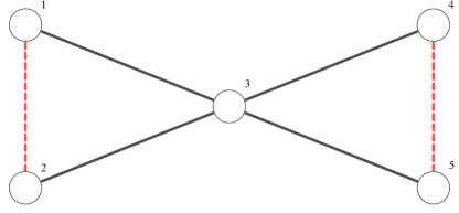
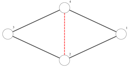
Figure 2: The two graphs referenced in Example 2.18.

The second graph has only one circuit of mixed type. The cycles $4\rightarrow 2\rightarrow 1\rightarrow 4$ and $4\rightarrow 3\rightarrow 2\rightarrow 4$ sum to $4\rightarrow 3\rightarrow 2\rightarrow 1\rightarrow 4$. Since this is a circuit of all positive edges it is in the kernel of $\partial$ and thus the second circuit is the inverse of the first. This gives the additive group as vectors of the form $k(0,1,0,-1)$.

Lemma 2.19

The flexibility

$$\tau=N+1-c(\Gamma_{+})-c(\Gamma_{-})$$

is equal to the the dimension of the group of cycles of mixed type.

Proof. This is a straightforward application of the Mayer-Vietoris sequence [34, §25]. We have the exact sequence

$$H_{1}({\Gamma})\overset{\partial}{\rightarrow}H_{0}({{\Gamma}_{+}}\cap{{\Gamma}_{-}})\overset{\alpha}{\rightarrow}H_{0}({{\Gamma}_{+}})\oplus H_{0}({{\Gamma}_{-}})\overset{\beta}{\rightarrow}H_{0}({\Gamma}).$$

The graph is assumed to be connected so $\dim(H_{0}({\Gamma}))=1$, $\dim(H_{0}({{\Gamma}_{+}})\oplus H_{0}({{\Gamma}_{-}}))=c({{\Gamma}_{+}})+c({{\Gamma}_{-}})$ and, since ${{\Gamma}_{+}}$ and ${{\Gamma}_{-}}$ have no common edges, $\dim(H_{0}({{\Gamma}_{+}}\cap{{\Gamma}_{-}}))=N$. The exactness implies that $\dim(\ker(\beta))=\dim(\mathop{\rm im}\nolimits(\alpha))=c({{\Gamma}_{+}})+c({{\Gamma}_{-}})-1$ and $\dim(\mathop{\rm im}\nolimits(\partial))=\dim(\ker(\alpha))=N-(c({{\Gamma}_{+}})+c({{\Gamma}_{-}})-1)=N+1-c({{\Gamma}_{+}})-c({{\Gamma}_{-}}).$ Note that the last quantity is exactly the flexibility. Thus the flexibility is equal to the number of linearly independent cycles of mixed type.

$\blacksquare$

This construction shows that the dimension of the group of mixed cycles is equal to the number of eigenvalues which cross from the left to the right-half plane. It would be more satisfying to give an explicit bijection between the basis of mixed cycles in the graph and the eigenvalues which cross over, or the associated eigenspaces. Of course we cannot really expect a bijection, since the eigenspace is an analytical object that depends sensitively on the edge weights, whereas the group of mixed cycles is topological and doesn’t depend on the edge weights. Nevertheless, there is a sort of topological stand-in for the eigenspace which nicely characterizes the modes which do not cross over. First we make a definition.

Definition 2.20

Let $S$ be a subspace (chosen independently of the weights $\gamma_{ij}$) and $P_{S}$ be the orthogonal projection onto the subspace $S$. The subspace $S$ is said to be a subspace of fixed index if the matrix

$$P_{S}{\mathcal{L}}:S\mapsto S$$

has the same index regardless of the choice of weights. A subspace of fixed index is maximal if

$$\dim(S)=c({{\Gamma}_{+}})+c({{\Gamma}_{-}})-1.$$

It is a simple consequence of the Courant minimax principle that the projection of a symmetric matrix onto a subspace cannot have more positive or more negative eigenvalues than the original operator. We know from theorem (2.8) that for appropriate choices of the weights the matrix can have as few as $c({{\Gamma}_{+}})-1$ negative eigenvalues and (for a different choice of weights) $c({{\Gamma}_{-}})-1$ positive eigenvalues. It thus follows that a subspace of fixed index cannot have more than $c({{\Gamma}_{+}})-1$ negative eigenvalues, $c({{\Gamma}_{-}})-1$ positive eigenvalues and one zero eigenvalue, and that the maximum possible dimension of a fixed subspace is $c({{\Gamma}_{+}})+c({{\Gamma}_{-}})-1.$ However it is not clear that one can actually have a maximal subspace of fixed index or, for that matter, any non-trivial subspace of fixed index at all. We conclude this section by showing that there is always a maximal subspace of fixed index that has a natural topological construction. In essence this subspace gives a natural (orthogonal) decomposition into modes which do not have an eigenvalue crossing, and modes which do.

First we need to define two complementary subspaces, one of which will be a maximal subspace of fixed index. The construction of these subspaces is similar in spirit to the construction of the cut-space and cycle-space from algebraic topology, although the cut-space and cycle-space are subspaces of the vector space over the edge set, not the vector space over the vertices. For a nice description of the cut- and cycle-space and some applications to the theory of electrical networks see the paper of Bryant [5].

Definition 2.21

Define $S_{\rm{free}}$ to be the following subspace of ${\mathbb{R}}^{N}:$ Given a basis for the mixed cycles $\{\gamma_{i}\}_{i=1}^{\tau}$ let $S_{{\rm free}}={\mathop{\rm span({\{v^{\gamma_{i}}\}_{i=1}^{\tau}.})}}$

Define $S_{\rm fixed}$ as follows: let ${{\Gamma}_{+}}_{i}$ be the $i^{th}$ component of $\Gamma_{+}$, and let $\vec{v}^{i,+}$ be the characteristic vector of ${{\Gamma}_{+}}_{i}$:

$$v^{i,+}_{j}=\begin{cases}1,&j\in\Gamma_{+,i},\\ 0,&j\not\in\Gamma_{+,i}.\end{cases}$$

Similarly, let $\vec{v}^{i,-}$ be the characteristic vector of ${{\Gamma}_{-}}_{i}$. Then

$$S_{\rm fixed}={\rm span}(\{v^{i,+}\}_{i=1}^{c(\Gamma_{+})},\{v^{i,-}\}_{i=1}^{c(\Gamma_{-})}).$$

Lemma 2.22

The subspaces $S_{\rm free}$ and $S_{\rm fixed}$ are orthogonal complements:

$$S_{\rm fixed}=S_{\rm free}^{\perp}$$

Proof. First we check that $\dim(S_{\rm fixed})=c(\Gamma_{+})+c(\Gamma_{-})-1$. Note that the set of vectors $\{\vec{v}^{i,+}\}$ is linearly independent, as is the set of vectors $\{\vec{v}^{i,-}\}$. However $\{\vec{v}^{i,+}\}\cup\{\vec{v}^{i,-}\}$ is not a linearly independent set, as one has

$$\sum_{i=1}^{c({{\Gamma}_{+}})}\vec{v}^{i,+}=\sum_{i=1}^{c({{\Gamma}_{-}})}\vec{v}^{i,-}=(1,1,1,\ldots,1).$$

We claim that this is the only relation. To see this note that we have the following identity for subspaces $Q,R$

$$\dim({\rm span}(Q\cup R))=\dim(Q)+\dim(R)-\dim({\rm span}(Q\cap R)).$$

Next note that ${\rm span}(\{\vec{v}^{i,+}\})\cap{\rm span}(\{\vec{v}^{i,-}\})$ consists of all vectors that are constant on components of $\Gamma_{+}$ and constant on components of $\Gamma_{-}$. Since $\Gamma$ is connected this means that these vectors must be constant on all of $\Gamma$, and are thus proportional to $(1,1,1,\ldots,1).$ It is clear that a basis for $S_{\rm free}$ is given by any $c(\Gamma_{+})+c(\Gamma_{-})-1$ vectors from $\{\vec{v}^{i,+}\}\cup\{\vec{v}^{i,-}\}.$

Next note that if $\gamma$ is a mixed cycle, with $\vec{v}^{\gamma}$ the corresponding vector, and $\vec{v}$ is constant on a component $\Gamma_{+,i}$, then

$$\langle\vec{v}^{\gamma},\vec{v}\rangle=0.$$

To see this first note that the number of times the cycle $\gamma$ enters $\Gamma_{+,i}$ must equal the number of times it leaves $\Gamma_{+,i}.$ When it enters and leaves $\Gamma_{+,i}$ it must do so through a negative edge. Each time it enters $\Gamma_{+,i}$ gives a $+1$ in some entry of $\vec{v}^{\gamma}$, and each time it leaves gives a $-1$ entry. Thus $\langle\vec{v}^{\gamma},\vec{v}\rangle$ is the sum of an equal number of $+1$ and $-1$ entries and is therefore zero.

Since $S_{\rm fixed}$ and $S_{\rm free}$ are orthogonal and have complementary dimensions they are orthogonal complements of one another. $\blacksquare$

Definition 2.23

We define the following subspaces of $S_{\rm fixed}$

• $S_{\rm fixed}^{+}=\{w|w\in{\rm span}\{v^{i+}\}_{i=1}^{c({{\Gamma}_{+}})}~{}~{}{\rm and}~{}~{}\langle w,(1,1,\ldots,1)\rangle=0\}$

• $S_{\rm fixed}^{-}=\{w|w\in{\rm span}\{v^{i-}\}_{i=1}^{c({{\Gamma}_{+}})}~{}~{}{\rm and}~{}~{}\langle w,(1,1,\ldots,1)\rangle=0\}$

• $S_{\rm fixed}^{0}={\rm span}((1,1,1,\ldots,1))$

Lemma 2.24

The subspaces $S_{\rm fixed}^{+/-/0}$ are ${\mathcal{L}}$–orthogonal. Specifically, what we mean by this is if $v$ and $w$ are chosen from two different subspaces of $S_{\rm fixed}^{+}$, $S_{\rm fixed}^{-}$, $S_{\rm fixed}^{0}$, then

$$\langle v,{\mathcal{L}}w\rangle=0.$$

Proof. $S_{\rm fixed}^{0}\subset\ker({\mathcal{L}})$, so the fact that any inner product involving that subspace is obvious. Thus we restrict our attention to $S_{\rm fixed}^{\pm}$. By definition $\vec{v}^{i^{\prime},-}$ is constant on the component $\Gamma_{i^{\prime},-}$ and zero off of this component. Let $\partial\Gamma_{i^{\prime},-}$ denote the set of vertices which are not in $\Gamma_{i^{\prime},-}$ but which are connected to it by a positive edge: the nearest neighbors of the component. By direct computation it is easy to see that ${\mathcal{L}}\vec{v}^{i^{\prime},-}$ takes the following form:

$$({\mathcal{L}}\vec{v}^{i^{\prime},-})_{j}=\left\{\begin{array}[]{c}-\sum_{k\in\partial\Gamma_{i^{\prime},-}}\gamma_{k,j}\qquad j\in\Gamma_{i^{\prime},-}\\ \sum_{k\in\Gamma_{i^{\prime},-}}\gamma_{k,j}\qquad j\in\ \partial\Gamma_{i^{\prime},-}.\end{array}\right.$$

Thus ${\mathcal{L}}\vec{v}^{i^{\prime},-}$ is a linear combination of vectors that are $1$ on some vertex in $\Gamma_{i^{\prime},-}$ and $-1$ on some vertex not in $\Gamma_{i^{\prime},-}$ but connected to it by a positive edge. Each of these vectors is necessarily orthogonal to $\vec{v}^{i,+}$ since $\vec{v}^{i,+}$ is constant on components of $\Gamma_{+}$. $\blacksquare$

We need one more lemma to prove the final result, the well-known Sylvester theorem

Lemma 2.25 (Sylvester’s law of Inertia)

If $A$ is a square matrix and $S$ a square non-singular matrix then $A$ and $B=S^{\dagger}AS$ have the same index. The matrices $A$ and $B$ are said to be Sylvester equivalent.

Proof. This is an old result and many proofs are known. We include a short one here for completeness. Consider the one-parameter family of Hermitian matrices $A(s)=(\cos(s)I-i\sin(s)B^{\dagger})A(\cos(s)I+i\sin(s)B^{\dagger}).$ The matrices $(\cos(s)I-i\sin(s)B^{\dagger})$ and $(\cos(s)I+i\sin(s)B^{\dagger})$ are both invertible, so $\dim(\ker(A(s))$ is independent of $s$, and there are no eigenvalue crossings. This gives a homotopy from $A(0)=A$ to $A(\frac{\pi}{2})=B^{\dagger}AB$ that does not change the index, so the indices of the two must be equal. $\blacksquare$

Proposition 2.26

The subspace $S_{\rm fixed}$ is a maximal subspace of fixed index: The operator $P_{S_{\rm fixed}}{\mathcal{L}}$ (considered as an operator from $S_{\rm fixed}$ to $S_{\rm fixed}$) has index

$$\mathop{\rm ind}\nolimits(P_{S_{\rm fixed}}{\mathcal{L}})=(c(\Gamma_{+})-1,1,c(\Gamma_{-})-1)$$

independent of the choice of edge weights.

Proof. Using Lemma 2.24 it follows that $P_{S_{\rm fixed}}{\mathcal{L}}$ has the following block structure:

$$P_{S_{\rm fixed}}{\mathcal{L}}P_{S_{\rm fixed}}={\mathcal{L}}_{-}\oplus{\mathcal{L}}_{0}\oplus{\mathcal{L}}_{+}$$

where ${\mathcal{L}}_{+}=P_{S_{\rm fixed}^{+}}{\mathcal{L}}$, ${\mathcal{L}}_{-}=P_{S_{\rm fixed}^{-}}{\mathcal{L}}$ and ${\mathcal{L}}_{0}=P_{S_{\rm fixed}^{0}}{\mathcal{L}}=0.$

Consider the block ${\mathcal{L}}_{-}\oplus{\mathcal{L}}_{0}$. This arises by orthogonal projection of ${\mathcal{L}}$ onto the set of vectors constant on ${{\Gamma}_{-}}$, and thus this matrix is Sylvester equivalent to the following graph Laplacian: one contracts on the negative edges, giving a graph with vertices corresponding to the components of ${{\Gamma}_{-}}$. This is a standard graph Laplacian on a connected graph with $c({{\Gamma}_{-}})$ vertices and thus has $c({{\Gamma}_{-}})-1$ negative eigenvalues and one zero eigenvalue. Similarly ${\mathcal{L}}_{0}\oplus{\mathcal{L}}_{+}$ is Sylvester equivalent to the negative of the graph Laplacian given by contracting on the positive edges. This has, by the same argument, $c({{\Gamma}_{+}})-1$ positive eigenvalues and one zero eigenvalue. The zero eigenvalue is obviously counted twice in this argument, giving

$${\rm ind}\left(P_{S_{\rm fixed}}{\mathcal{L}}P_{S_{\rm fixed}}\right)=(c({{\Gamma}_{-}})-1,1,c({{\Gamma}_{+}})-1).$$

$\blacksquare$

3 Refinements

In this section, we present some refinements of Theorem 2.8. In Section 3.1 we present the Deletion-Contraction Theorem, which allows us to obtain recursive formulas for the $\mathcal{M}({\Gamma}(t))$ polynomial in terms of “smaller” graphs obtained by deleting and contracting edges; this allows us to give a precise characterization of the bifurcation structure of $\mathcal{L}({\Gamma}(t))$ in many cases. In Section 3.2, we discuss the asymptotics of the individual eigenvalues of $\mathcal{L}({\Gamma}(t))$ in the limits $t\to 0,\infty$. Recall that in the statement and proof of Theorem 2.8, we discuss the number of eigenvalues in the left- and right-hand half-planes in these two limits; here we give more precise statements of the locations of these eigenvalues.

3.1 Deletion–contraction theorem

Definition 3.1

Let ${\Gamma}=(V,E)$ be a weighted multigraph (loops and multiple edges allowed), and $e\in E({\Gamma})$ an edge. Let ${{\Gamma}}_{/{e}}$ denote the graph obtained by removing edge $e$: the graph with vertex set $V({\Gamma})$ and edge set $E({\Gamma})-e$. If $e$ is an edge which is not a loop let ${{\Gamma}}_{.{e}}$ denote the graph obtained by contracting on the edge, which is obtained as follows:

• If edge $e$ connects vertices $v_{1}$ and $v_{2}$ then $v_{1}$ and $v_{2}$ are identified as a single vertex $v^{*}$.

• Each edge connecting a vertex to $v_{1}$ or $v_{2}$ becomes an edge connecting that vertex to $v^{*}$

• Edge $e$ is removed from the edge set.

Note that if ${\Gamma}$ is a simple graph and $v_{1}$ and $v_{2}$ are part of a triangle then the contracted graph ${{\Gamma}}_{.{e}}$ will have multiple edges. Similarly if there are multiple edges connecting $v_{1}$ and $v_{2}$ then ${{\Gamma}}_{.{e}}$ will have loops.

We can now state the Deletion-Contraction Theorem.

Theorem 3.2 (Deletion-Contraction theorem)

Let ${\Gamma}$ be a weighted multigraph with $e\in E({\Gamma})$. Then $\mathcal{M}({\Gamma})$ can be computed by applying the following rules

• If $e$ is not a loop then $\mathcal{M}({\Gamma})=\mathcal{M}({{\Gamma}}_{/{e}})+\gamma_{e}\mathcal{M}({{\Gamma}}_{.{e}}).$

• If $e$ is a loop then $\mathcal{M}({\Gamma})=\mathcal{M}({{\Gamma}}_{/{e}}).$

• If ${\Gamma}$ is disconnected then $\mathcal{M}({\Gamma})=0$

Proof. The deletion-contraction recursion is well-known — see Chapter 13.2 of the text of Godsil and Royle [12] for one proof. $\blacksquare$

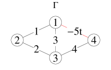
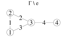
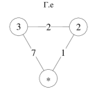
Figure 3: The graphs ${\Gamma};{\Gamma}\setminus e;{\Gamma}.e$, where $e$ is chosen to be the edge with negative weight.

Example 3.3

As an example, let us consider the graphs given in Figure 3 (here, think of the $t$ as a symbol to separate out the terms containing the special edge). First, notice that ${\Gamma}$ has three spanning trees not containing $e$, of weights $8,12,24$, and five spanning trees containing $e$, of weights $-10t,-15t,-20t,-30t,-40t$. By Lemma 2.6,

$$\mathcal{M}({\Gamma})=44-115t.$$

Notice that every spanning tree of ${\Gamma}$ that does not contain $e$ is also a spanning tree of ${\Gamma}\setminus e$, and thus

$$\mathcal{M}({\Gamma}\setminus e)=44.$$

On the other hand, $\Gamma.e$ has three spanning trees of weights $2,7,14$. Therefore we have

$$\mathcal{M}({\Gamma}.e)=23.$$

And we see that

$$\mathcal{M}({\Gamma})=44-115t=44+(-5t)(23)=\mathcal{M}({{\Gamma}}_{/{e}})-\gamma_{e}\mathcal{M}({{\Gamma}}_{.{e}}).$$

In the context of dynamical systems, an important distinction to be made is that between graphs for which $n_{+}(\mathcal{L}({\Gamma}))=0$ and those for which $n_{+}(\mathcal{L}({\Gamma}))>0$; the former are called stable and the latter unstable. This notion comes from the fact that if we consider the ordinary differential equation

$$\dot{x}=\mathcal{L}(G)x,$$

then the origin is stable to perturbations iff $n_{+}(\mathcal{L}(G))=0$; if not, then perturbations move away from the origin at an exponential rate.

Moreover, as proved above, when we consider the homotopy ${\Gamma}(t)={\Gamma}_{+}+t{\Gamma}_{-}$, the function $n_{+}(\mathcal{L}({\Gamma}(t)))$ is a non-decreasing function of $t$. From this, it follows that if we define

$$t^{\star}({\Gamma}):=\sup_{t\geq 0}n_{+}(\mathcal{L}({\Gamma}(t)))=0,$$

then for $t\leq t^{\star}({\Gamma})$, the Laplacian is stable, and for $t>t^{\star}({\Gamma})$, the Laplacian is unstable—in short, it undergoes a dynamical bifurcation.

Two facts follow immediately from Theorem 2.8: first, that $t^{\star}({\Gamma})>0$ if and only if ${\Gamma}_{+}$ is connected, and $t^{*}({\Gamma})<\infty$ if and only if ${\Gamma}_{-}\neq 0$. We will concentrate the most in what follows on the case of $t^{\star}({\Gamma})\in(0,\infty)$.

We also point out that rigid graphs undergo no bifurcation; in fact $n_{+}({\Gamma}(t))$ is constant on $\{t>0\}$. From the bifurcation point of view, then, these are the least interesting cases.

We now work out some special cases.

3.1.1 One negative edge

Let us first consider the case where ${{\Gamma}_{+}}$ is connected, and there is exactly one negative edge in ${{\Gamma}_{-}}$, call it $e$. Then we have

$$\mathcal{M}({\Gamma}(t))=\mathcal{M}({{\Gamma}_{+}})-t\left|{\gamma_{e}}\right|\mathcal{M}({\Gamma}.e).$$

This means that

$$t^{\star}=\frac{\mathcal{M}({{\Gamma}_{+}})}{\left|{\gamma_{e}}\right|\mathcal{M}({\Gamma}.e)}.$$

Notice that this formula gives $t^{\star}>0$; since ${{\Gamma}_{+}}$ and ${\Gamma}.e$ have non-negative entries, they will have opposite signs, since their dimensions differ by one (q.v. (2.3)).

Intuitively, we expect that the denser a graph is, the less powerful each individual edge would be. We present a couple of examples.

Example 3.4 (Ring graph)

Consider the case of the ring graph $R_{N}$, i.e. $V(R_{N})=\{1,\dots,N\}$ and

$$(R_{N})_{ij}=\begin{cases}1,&j=i\pm 1\pmod{N},\\ 0,&\mbox{else.}\end{cases}$$

We also define the path graph $P_{N}=R_{N}\setminus\{1,N\}$. Choose any edge of $R_{N}$ and flip its sign to minus one. According to the Proposition above, the homotopy $\mathcal{L}({\Gamma}(t))$ will lose stability at

$$t^{\star}=\frac{\mathcal{M}(\Gamma\setminus e)}{\mathcal{M}(\Gamma.e)}=\frac{\mathcal{M}(P_{N})}{\mathcal{M}(R_{N-1})}.$$

It is easy to see that $\mathcal{M}(R_{N})=N,\mathcal{M}(P_{N})=1$, so we have

$$t^{*}=\frac{1}{N-1}.$$

Example 3.5 (Complete graph)

Consider the complete graph $K_{N}$. Again choose any edge, then the deletion operators give graphs $OG_{N},DR_{N-1}$. $OG_{N}$ is the complete graph minus one edge; $DR_{N}$ is a complete graph on $N$ nodes with all of the edges going to one distinguished vertex having twice the weight.

Using standard counting arguments, we see that

$$\mathcal{M}(OG_{N})=(N-2)N^{N-3},\quad\mathcal{M}(DR_{N})=2(N+1)^{N-2},$$

giving

$$t^{\star}=\frac{\mathcal{M}(OG_{N})}{\mathcal{M}(DR_{N-1})}=\frac{(N-2)N^{N-3}}{2N^{N-3}}=\frac{N-2}{2}.$$

Of course, this can be obtained by other means; in fact, one can compute that the eigenvalues of ${\Gamma}(t)$ are

$$\{0\}\cup\{-N\}^{(N-2)}\cup\{2t+(N-2)\},$$

and the computation would also follow from this.

Conjecture 3.6

These are the extreme cases; for any graph $\Gamma$ with ${{\Gamma}_{+}}$ connected and $\left|{E({{\Gamma}_{-}})}\right|=1$, we have

$$t^{\star}(\Gamma)\in[(N-1)^{-1},(N-2)/2].$$

Proposition 3.7

Assume that $\left|{E({{\Gamma}_{-}})}\right|=2$ and that the two edges $e,f\in E({{\Gamma}_{-}})$ do not share a vertex. Then

$$\mathcal{M}({\Gamma}(t))=t^{2}\left|{\gamma_{e}\gamma_{f}}\right|\mathcal{M}({{\Gamma}}_{.{e}.{f}})-t\left(\left|{\gamma_{e}}\right|\mathcal{M}({{\Gamma}}_{.{e}\setminus{f}})+\left|{\gamma_{f}}\right|\mathcal{M}({{\Gamma}}_{\setminus{e}.{f}})\right)+\mathcal{M}({{\Gamma}}_{\setminus{e}\setminus{f}}),$$

where we have defined all of these terms in Definition 3.1. Also, $t^{*}(\Gamma)$ is the minimal positive root of this polynomial.

Proof. Let $\Gamma$ be any signed graph; from Theorem 3.2, we have

$$\mathcal{M}({\Gamma})=\gamma_{e}\mathcal{M}({{\Gamma}}_{.{e}})+\mathcal{M}({{\Gamma}}_{/{e}}),$$

and

$$\mathcal{M}({{\Gamma}}_{.{e}})=\gamma_{f}\mathcal{M}({({{\Gamma}}_{.{e}})}_{.{f}})+\mathcal{M}({({{\Gamma}}_{.{e}})}_{/{f}}),\quad\mathcal{M}({{\Gamma}}_{/{e}})=\gamma_{f}\mathcal{M}({({{\Gamma}}_{/{e}})}_{.{f}})+\mathcal{M}({({{\Gamma}}_{/{e}})}_{/{f}}),$$

and iterating (• ‣ 3.2) gives

$$\mathcal{M}({\Gamma})=\gamma_{e}\gamma_{f}{{\Gamma}}_{.{e}.{f}}+\gamma_{e}\mathcal{M}({{\Gamma}}_{.{f}\setminus{e}})+\gamma_{f}\mathcal{M}({{\Gamma}}_{.{e}\setminus{f}})+\mathcal{M}({{\Gamma}}_{\setminus{e}\setminus{f}}).$$

If the edges $e$ and $f$ are in $E({\Gamma}_{-})$, then $\gamma_{e}=-t\left|{\gamma_{e}}\right|,\gamma_{f}=-t\left|{\gamma_{f}}\right|$, and the result follows. $\blacksquare$

Remark 3.8

Note that this polynomial has positive roots by Theorem 2.8. Consider, for example, an unweighted graph; this implies (q.v. Remark 2.14) that

$$\left(\mathcal{M}(\Gamma.e\setminus f)+\mathcal{M}(\Gamma\setminus e.f)\right)^{2}>4\mathcal{M}(\Gamma.e.f)\mathcal{M}(\Gamma\setminus e\setminus f).$$

3.2 Detailed Eigenvalue Asymptotics

We now consider more detailed asymptotics of the eigenvalue spectrum in the limits in which the strength of the negative edges is much weaker or much stronger than the strength of the positive edges. Specifically we consider the one-parameter family of graph Laplacians

$$\mathcal{L}({\Gamma}(t))=\mathcal{L}({{\Gamma}_{+}})-t\mathcal{L}({{\Gamma}_{-}}),$$

in the limits $t\rightarrow 0^{+}$ and $t\rightarrow\infty$. The spectrum splits naturally into two parts, which correspond to the eigenvalues of graph Laplacians on the deleted and contracted graphs. This is an analog on the level of the spectrum of the contraction-deletion algorithm for computing the crossing polynomial: the crossing polynomial is given by the sum of the crossing polynomials for the contracted and deleted graphs, while the spectrum is given (asymptotically!) by the union of the deleted and contracted graphs.

Theorem 3.9

Suppose that $t$ is large and positive. Then ${\mathcal{L}}(t)$ has exactly $N-c({{\Gamma}_{-}})$ negative eigenvalues, $c({{\Gamma}_{-}})-1$ positive eigenvalues and one zero eigenvalue. If we take the convention that eigenvalues are numbered in decreasing order then to leading order in $t$ the $c({{\Gamma}_{-}})-1$ positive eigenvalues are given by

$$\lambda_{i}(\mathcal{L}_{\Gamma})=t\lambda_{i}(\mathcal{L}_{\Gamma_{-}})+O(1)\qquad\qquad i\in\{1\ldots c({{\Gamma}_{-}})-1\},$$

The $N-c({{\Gamma}_{-}})$ negative eigenvalues are given to leading order by

$$\lambda_{i}(\mathcal{L}_{\Gamma})=\tilde{\lambda}_{i}(\mathcal{L}_{\Gamma\cdot-})+o(1)\qquad\qquad i\in\{N\ldots c({{\Gamma}_{-}})+1\},$$

where $(L_{\Gamma\cdot-}$ is the graph formed by contracting on the negative edges. Here $\tilde{\lambda}_{j}(\mathcal{L}_{\Gamma\cdot-})$ are solutions to

$$\mathcal{L}_{\Gamma^{-}}\vec{v}=\lambda S\vec{v}$$

where $L_{\Gamma^{-}}$ is the graph Laplacian formed by contracting on the negative edges and $S$ the contracted inner product: the diagonal matrix with entries $S_{ii}=|V(\Gamma_{-,i})|$.

Proof. The proof follows in a straightforward way from perturbation theory for eigenvalues of a symmetric matrix. The full graph Laplacian can be written

$${\mathcal{L}}(t)=t\left({\mathcal{L}}(\Gamma_{-})+t^{-1}{\mathcal{L}}(\Gamma_{+})\right)$$

so it suffices to understand the eigenvalues of ${\mathcal{L}}(\Gamma_{-})+t^{-1}{\mathcal{L}}(\Gamma_{+})$ for $t$ large. The spectrum of ${\mathcal{L}}(\Gamma_{-})$ consists of $c(\Gamma_{-})$ zero eigenvalues and $N-c(\Gamma_{-})$ positive eigenvalues. For the non-zero eigenvalues straightforward eigenvalue perturbation theory gives the asymptotic above.

To understand how the $c(\Gamma_{-})$-dimensional kernel breaks under perturbation we must do a degenerate perturbation theory calculation. Well-known results (again see Kato) show that to leading order the eigenvalues are given by the eigenvalues of the reduced matrix

$$P_{\ker({\mathcal{L}}_{-})}L_{\Gamma_{+}}P_{\ker({\mathcal{L}}_{-})}$$

where $P_{\ker({\mathcal{L}}_{-})}$ is the orthogonal projection onto the kernel of ${\mathcal{L}}_{-}$. It is straightforward to compute $\ker({\mathcal{L}}_{-})$: it consists of vectors that are constant on components of ${\mathcal{L}}_{-}$. We can identify a vector $\vec{w}\in\ker({\mathcal{L}}_{-})$ with a vector $\tilde{w}\in{\mathbb{R}}^{c(\Gamma_{-})}$ by the following rule: if $w_{i}=\alpha$ for all vertices in component $\Gamma_{-},j$ then $\tilde{w}_{j}=\alpha$. Under this identification the natural inner product on ${\mathbb{R}}^{N}$ maps to the inner product

$$\langle\tilde{v},\tilde{w}\rangle=\sum_{i=1}^{c(\Gamma_{-})}|V(\Gamma_{i,-})|\tilde{v}_{i}\tilde{w}_{j}.$$

In other words the there is one entry per component of $\Gamma_{-}$, and the inner product is diagonal with weights given by the number of vertices in the corresponding component of $\Gamma_{i}.$ It is straightforward to see that the matrix

$$P_{\ker({\mathcal{L}}_{-})}L_{\Gamma_{+}}P_{\ker({\mathcal{L}}_{-})}$$

is exactly the Laplace matrix obtained by contracting on the negative edges of the graph, completing the proof. $\blacksquare$

Definition 3.10

Given a matrix $A$, we define ${\mathrm{Spec}}^{\star}(A)$ as the eigenvalues of the matrix $A$ restricted to the subspace $(1,1,1,\ldots,1)^{\perp}$ of mean zero vectors.

Remark 3.11

The previous theorem can be written in the following compact way

$${\mathrm{Spec}}^{\star}({\mathcal{L}}(t))\approx\left\{\begin{array}[]{c}\ {\mathrm{Spec}}^{\star}({{\Gamma}_{-}})\cup{\mathrm{Spec}}^{\star}({\Gamma}_{\cdot-})\qquad t\rightarrow+\infty\\ {\mathrm{Spec}}^{\star}({{\Gamma}_{+}})\cup{\mathrm{Spec}}^{\star}({\Gamma}_{\cdot+})\qquad t\rightarrow 0^{+}\par\end{array}\right.$$

with the understanding that the eigenvalues for the contracted graph are taken with respect to the natural inner product $S$. This shows that there is an (approximate) contraction-deletion relation at the level of the spectrum analogous to the contraction-deletion relation satisfied by the crossing polynomial.

Example 3.12

We consider the following graph, where all positive (solid) edges are weighted $+1$ and all negative (dashed) edges weighted $-1$:

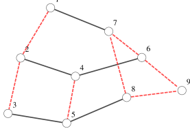
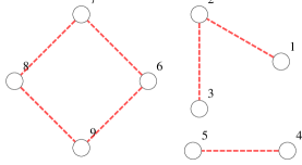
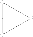
Figure 4: The graph ${\Gamma}$; the graph ${{\Gamma}_{-}}$; the graph ${\Gamma}_{\cdot-}$

The full graph has five positive edges, seven negative edges and nine vertices. The subgraph $\Gamma_{-}$ consisting of only the negative links has three components. Component A consists of vertices 1,2 and 3 and connecting edges , component B consists of vertices 4 and 5 and the connecting edge, and Component C consists of vertices 6, 7, 8, and 9 and connecting edges. There are $N-c({{\Gamma}_{-}})=9-3=6$ non-zero eigenvalues corresponding to the graph Laplacian associated with the negative edges. The non-zero eigenvalues associated to component A are $1$ and $3$, to component B is $2$ and to component C are $4$, $2$ and $2$. This gives six eigenvalues that grow linearly:

$$\lambda_{9}\approx 4t+O(1)$$

$$\lambda_{8}\approx 3t+O(1)$$

$$\lambda_{7}\approx 2t+O(1)$$

$$\lambda_{6}\approx 2t+O(1)$$

$$\lambda_{5}\approx 2t+O(1)$$

$$\lambda_{4}\approx 1t+O(1)$$

If one contracts on all of the dashed edges the full graph reduces to the three cycle, with one vertex corresponding to each component of ${{\Gamma}_{-}}$. There are two edges between components A and B, two between components B and C, and one between A and C, so these edges are weighted accordingly. The norm is contracted as well, and the norm over the new vertex space can be written as

$$\|\vec{v}\|^{2}=\vec{v}^{t}S\vec{v}$$

where $S$ is the matrix

$$S=\left(\begin{array}[]{ccc}3&0&0\\ 0&2&0\\ 0&0&4\end{array}\right)$$

The diagonal entries reflect the fact that the components have three, two and four vertices respectively. Thus the eigenvalue problem becomes

$$\left(\begin{array}[]{ccc}-3&2&1\\ 2&-4&2\\ 1&2&-3\end{array}\right)\vec{v}=\lambda\left(\begin{array}[]{ccc}3&0&0\\ 0&2&0\\ 0&0&4\end{array}\right)\vec{v}$$

giving the negative eigenvalues as

$$\lambda_{2}(t)\approx\frac{1}{8}\left(\sqrt{33}-15\right)+O({1}/{t})$$

$$\lambda_{1}(t)\approx\frac{1}{8}\left(-\sqrt{33}-15\right)+O({1}/{t})$$

Finally the flexibility is equal to $\tau({\Gamma})=10-3-4=3$, so there are three eigenvalue crossings. It is straightforward though tedious to compute that the crossing polynomial is given by $P_{\Gamma}(t)=171t^{3}-702t^{4}+828t^{5}-288t^{6}.$ The non-zero roots occur at $t\approx.43,t\approx.90,t\approx 1.55$.

Some numerical results are shown in Figure . The first plot shows a graph of $\lambda_{i}(t)/t$ for $i=3\ldots 9$ and $t\in(0,8).$ It seems clear that the scaled eigenvalues are converging to the correct values. The second plot shows a plot of the (unscaled) negative eigenvalues for $t\in(0,8).$ Again it is clear that they are converging to $-\frac{1}{8}(\sqrt{33}+15)$ and $-\frac{1}{8}(15-\sqrt{33})$ respectively. One can also see that there are three eigenvalue crossings at the correct $t$ values.

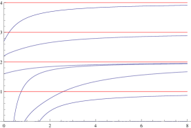
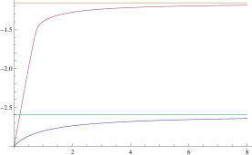
Figure 5: Eigenvalues of ${\Gamma}(t)$ as a function of $t$, where ${\Gamma}(t)$ is defined in Example 3.12.

3.3 Comparison to the Gershgorin Theorem

In applied mathematics and numerical analysis it is often necessary to estimate the locations of the eigenvalues of a matrix or linear operator. One simple and very widely used tool for this is the Gershgorin disc theorem, which says the following:

Theorem 3.13 (Gershgorin)

Given a matrix $M$ with entries $M_{ij}$ define the following $n$ closed disks:

$$D_{i}=\{z||z-M_{ii}|\leq\sum_{j\neq i}|M_{ij}|\}.$$

Then the eigenvalues of $M$ lie in the union of the disks, ${\rm spec}(M)\in\cup_{i=1}^{n}D_{i}.$

The fact that the disks are defined using the edge weights might make one think that the Gershgorin theorem might give more information on the signs of the eigenvalues than the purely topological arguments, but this is not, in fact, the case. It is not difficult to see that, for a non-trivial signed Laplacian the Gershgorin theorem always gives results that are strictly worse than those given by Theorem 2.8.

First note that if the matrix $M$ represents a graph Laplacian then there are three kinds of discs. If all of the edges emanating from the vertex are all positive (resp. all negative) then the associated disc lies in the closed left half-plane (resp. right half-plane) and is tangent to the origin and the corresponding eigenvalue is non-positive (resp. non-negative). If the vertex has edges of both signs then the origin lies in the interior of the disk and the sign of the eigenvalue cannot be determined. It is these discs that correspond to eigenvalues whose sign cannot be determined. The main observation in this section is that the number of such discs is always strictly larger than $\tau.$

Proposition 3.14

Suppose the graph ${\Gamma}$ is connected and contains edges of both signs. Let $n$ be the number of Gershgorin discs for which the origin lies in the interior. Then $n\geq\tau+1$.

Proof. This follows immediately from the topological characterization of the number of of modes for which there is an eigenvalue crossing. The results of the previous section show that these can be associated with mixed cycles. By the construction given in that section we associate to each of these cycles a vector that has $+1$ for each time the cycle enters a vertex from a positive edge and leaves it by a negative edge, and $-1$ for each time the cycle enters a vertex from a negative edge and leaves it by a positive edge. These vectors can only have non-zero entries in vertices which have both types of edge, so they obviously lie in a subspace isomorphic to ${\mathbb{R}}^{n}$. These vectors are necessarily orthogonal to $(1,1,1,\ldots,1)$, so there can be at most $n-1$ linearly independent ones. $\blacksquare$

Remark 3.15

Note that $n=\tau+1$ can be achieved — one example is when $c({{\Gamma}_{+}})=1$ and $c({{\Gamma}_{-}})=1$, when $\tau=N-1$ and $n=N$. It can also happen that $n$ is much larger than $\tau$. Consider, for example, an even cycle with edges of alternating sign. In this case $n=N$ — all vertices have edges of both type — while $\tau=1$ since there is only one linearly independent loop.

Example 3.16

The graph depicted in Figure 4 has a flexibility of $\tau=9+1-4-3=3$. This graph has eight vertices which have edges of both signs, and thus eight Gershgorin discs that contain the origin in the interior.

In the second graph in figure 1 there are three vertices that have edges of both types, and thus three Gershgorin discs that contain the origin as an interior point. The flexibility of this graph, however, is zero so that the number of positive, negative and zero eigenvalues is fixed and does not vary with the edge weights.

4 Applications and numerical computations

4.1 Random graphs and bifurcations

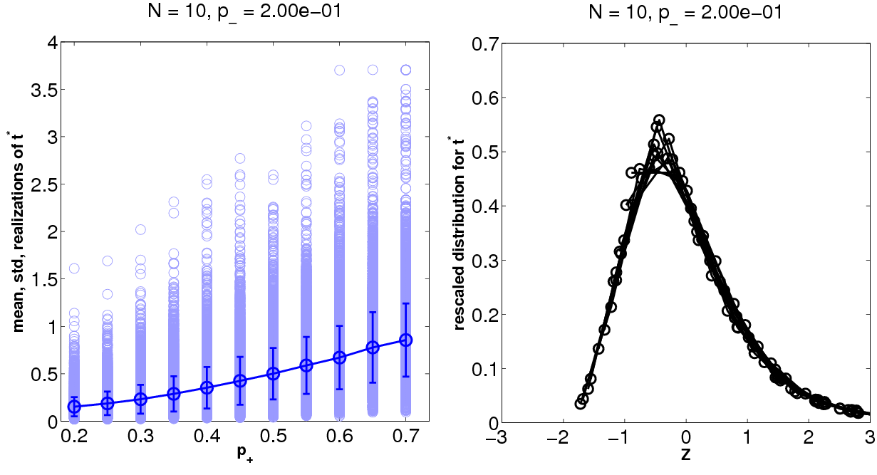
Figure 6: Each of the rows corresponds to a fixed $N$; the top row is $N=10$ and the bottom row is $N=50$. In each row, in the left panel, we plot in solid blue the mean and standard deviation for ensembles of random matrices where we vary $p_{+}$, and in light blue, we plot the value of $t^{\star}$ for each individual matrix. In the right panel, we have plotted the distributions for all values of $p_{+}$, but rescaled to have mean zero and variance one. For the case of $N=50$, we compare these rescaled distributions to the standard Gaussian.

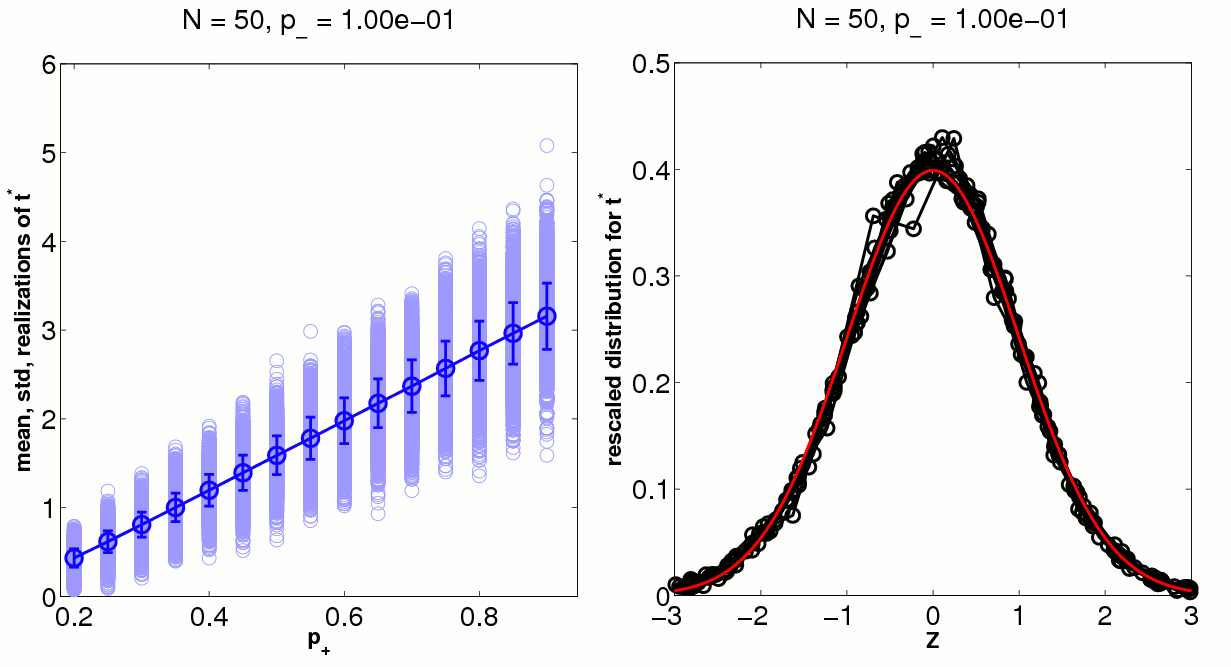
Figure 7: In the left panel, in solid blue we plot the mean and standard deviation for an ensemble of random matrices with a given $p_{+}$, $p_{-}=0.1$, and $N=50$, versus $p_{+}$. In light blue, we plot the value of $t^{\star}$ for each individual matrix. In the right, we have plotted the distributions for all values of $p_{+}$, but rescaled to have mean zero and variance one. We compare with the Gaussian in red.

It was shown in Section 3.1 that for any signed $\Gamma$,

$$t^{\star}:=\sup_{t\geq 0}\{t:n_{+}({\Gamma}(t))=0\}$$

satisfies $t^{\star}\in[0,\infty]$, and that $t^{\star}=0$ if and only if ${{\Gamma}_{+}}$ is not connected, and $t^{\star}=\infty$ if and only if ${{\Gamma}_{-}}=0$. Thus we can think of $t^{\star}$ as a map from the set of finite graphs to $[0,\infty]$. For any collection $\mathcal{G}$ of graphs and a probability measure $\mathbb{P}$ on $\mathcal{G}$, this induces a random variable $T\colon\mathcal{G}\to[0,\infty]$.

We present some numerically-computed distributions in Figure 6 and 7 below. The random ensemble of matrices is a signed generalization of the classical Erdős–Rényi random graph $G(n,p)$ whose specific definition is given as follows: we fix $N$ and $p_{\pm}\in[0,1]$. For each $1\leq i<j\leq N$, choose $X_{ij},Y_{ij}$ independently, with

$$\mathbb{P}(X_{ij}=1)=p_{+},\quad\mathbb{P}(X_{ij}=0)=1-p_{+},\quad\mathbb{P}(Y_{ij}=1)=p_{-},\quad\mathbb{P}(Y_{ij}=0)=1-p_{-},$$

and we set $\gamma_{ij}=X_{ij}-Y_{ij}$. From this, we have

$$\mathbb{P}(\gamma_{ij}=+1)=p_{+}(1-p_{-}),\quad\mathbb{P}(\gamma_{ij}=-1)=p_{-}(1-p_{+}),$$

and $\gamma_{ij}=0$ otherwise, and of course the $\gamma_{ij}$ are independent as well. We then set $\gamma_{ij}$ with $i>j$ by symmetry. This gives a random distribution on the set of symmetric graphs with $N$ vertices. We condition on ${{\Gamma}_{+}}$ being connected and ${{\Gamma}_{-}}\neq 0$, and then compute the distribution of $t^{\star}$ over this ensemble.

We performed a series of numerical experiments on these random variables, both for $N=10$ (“small matrices”) and $N=50$ (“large matrices”), the numbers 10 and 50 being chosen arbitrarily. In each of these cases, we fixed $p_{-}$ for all simulations (we chose $p_{-}=0.20$ for $N=10$ and $p_{-}=0.10$ for $N=50$) and varied $p_{+}$ over a range. For each choice of $p_{\pm}$, we chose a random ensemble of $10^{4}$ matrices using the rules above, and computed $t^{*}$ for each of the matrices in the ensemble using a bisection method. We present the findings in Figures 6 and 7. We first observe that $t^{*}$ tends to increase as $p_{+}$ increases, which makes sense: adding more positive edges will make the Laplacian more stable, and higher $p_{+}$ values tend to give more positive edges. What is perhaps surprising is that the ensemble mean is very close to a linear function of $p_{+}$ (at least for a certain range for $N=10$, and for all $p_{+}$ for $N=50$). Moreover, we find that there seems to be a universal scaling distribution for the different values of $p_{+}$; in each case, what we do is consider the distribution of $t^{*}$ for each choice of $p_{\pm}$, then normalize this distribution to have mean zero and variance one, and plot these on top of each other. For the small ($N=10$) case, the rescaled distributions overlap well and resemble a lognormal plot; for the $N=50$ case, the rescaled distributions overlap well and resemble a normal plot.

To make these observations more precise, in each case we chose $p_{+}=0.45$ and made a QQ-plot of the ensemble distribution versus either a lognormal (for $N=10$) or a normal (for $N=50$), and these match quite well. See Figure 8.

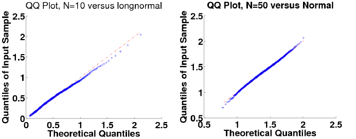
Figure 8: QQ-plots of ensemble distributions. In the left frame, we are plotting a QQ-plot of the ensemble distribution $N=10$, $p_{-}=0.20$, $p_{+}=0.45$ versus a lognormal; in the right frame, we plot the ensemble distribution for $N=50,p_{-}=0.10,p_{+}=0.45$ versus a normal.

4.2 Feuds in social networks

We consider two datasets from social networks and compute the flexibility of the graphs and, in one case, the bifurcations. Our computations were facilitated by the matlab_bgl library .

The first dataset we consider is from Read [37], and represents sympathetic and antagonistic relationships amongst sixteen sub-tribes of the Gahuku-Gama people in the highlands of New Guinea: Gaveve, Kotuni,Gama, Nagamidzhuha, Seu’ve, Kohika, Notohana, Uheto, Nagamiza, Masilakidzuha, Asarodzuha, Gahuku, Gehamo, Ove, Ukudzuha and Alikadzuha. Warfare between subtribes in this society was very common. While temporary alliances are common this dataset represents traditional relationships between subtribes. The positive, or hina, edges represent subtribes that are traditionally close politically. Warfare between these subtribes occurs but is limited. It is understood to be short term condition and is often resolved by payment of blood money or other concessions. The negative, or rova, edges represent relations between subtribes that are traditionally antagonistic. Warfare between these subtribes is much less constrained. This has become a somewhat popular data set to analyze: see the pioneering work of Hage and Harary [16] and the recent work of Kunegis et. al [28]. The graph has $c({{\Gamma}_{+}})=2$ and $c({{\Gamma}_{-}})=3$, giving $\tau=12$. The first component (A) of ${{\Gamma}_{+}}$ consists of a collection of four tribes (Gaveve, Kotuni,Gama, Nagamidzhuha; here numbered 1-4) all of whom have friendly relations. The second component (B) consists of the remaining twelve tribes (Seu’ve, Kohika, Notohana, Uheto, Nagamiza, Masilakidzuha, Asarodzuha, Gahuku, Gehamo, Ove, Ukudzuha and Alikadzuha; here numbered 5-16), all of whom are connected by at least one chain of sympathetic relationships. Relations are more complicated within component (B) than in component A but there are two main features to be noted. The first is that removing the Masilakidzuha (tribe number 10) splits this component into two subcomponents, the first subcomponent (B1) consisting of the Seu’ve, Kohika, Notohana, Uheto, Nagamiza and the second subcomponent (B2) consisting of the Asarodzuha, Gahuku, Gehamo, Ove, Ukudzuha and Alikadzuha. There are numerous antagonistic relationships between tribes in subcomponents B1 and subcomponent B2 but there are no antagonistic relationships within subcomponents B1 or B2. This suggests the possibility of a rift developing within component B.

The second dataset is from the Slashdot Zoo. Slashdot  is a user-run website where links are submitted and voted on by the userbase, and, furthermore, users can make comments on the links and these comments are also voted on by the individual users. A significant amount of discussion occurs on this website, sometimes friendly and sometimes fractious, and thus it is not hard to imagine that connections, both positive and negative, form between users. Each user is allowed to tag other users in the database as a “fan” or a “foe”, i.e. if user $i$ likes the types of comments made by user $j$, user $i$ has the possibility to tag user $j$ and become a “fan”. If this occurs, then in the Slashdot Zoo  database, the edge $(i,j)$ is given weight $+1$. Similarly, user $i$ can be a “foe” of user $j$ and this adds a $-1$ on edge $(i,j)$. This dataset contained connection data on 82,144 users, with 549,202 edges in the graph. This network is not a priori symmetric, since the fan/foe operations have directionality, so we imposed symmetry. Given users $i$ and $j$, if $i$ and $j$ are both fans of each other, or $i$ is a fan to $j$ and $j$ is neutral to $i$, then we placed a $+1$ in edge $(i,j)$. Similarly for foes, if $i$ and $j$ are both foes, or $i$ is a foe to $j$ and $j$ is neutral to $i$, then we placed a $-1$ in edge $(i,j)$. In short, we allowed simply extended unidirectional relationships to be bidirectional as long as the other direction was neutral. The only case to think about is what one should do if the two directions are of opposite sign, i.e. if $i$ was a fan of $j$ and $j$ a foe of $i$; in this case we decided to assume that the relationship canceled and placed a 0 on edge $(i,j)$. As one can imagine, this is relatively rare, and this happened only 1,949 times in this dataset.

Thus, in both cases, we are considering a network with positive and negative weights. Since it has a smaller vertex set, the PNG dataset was easier to analyze. We present this data in Figure 9. Since $c({{\Gamma}_{+}})=2$, and $\tau=12$ the results of Theorem 2.8 imply that we will have we will have

$$\lim_{t\to 0^{+}}n_{+}({\Gamma}(t))=1,\quad\lim_{t\to\infty}n_{+}({\Gamma}(t))=13.$$

A symbolic computation using Mathematica gives the crossing polynomial as

$${\mathcal{M}}(t) =-45432223t^{13}+657635624t^{12}-4187415940t^{11}+15505043366t^{10}-37159886129t^{9}$$

$$\quad+60647687776t^{8}-68960526571t^{7}+54844706645t^{6}-30103762121t^{5}+11015925656t^{4}$$

$$\quad-2508107376t^{3}+308319872t^{2}-14192640t.$$

The twelve positive roots of the crossing polynomial range from $t\approx.1$ to $t\approx 3$. For small positive $t$ we have one positive eigenvalue. This, of course, represents the mutual antagonism between the subtribes in component A and the subtribes in component B. The first bifurcation occurs around $t\approx.1$ when a secondary instability develops. Intuitively one expects that this corresponds to a split in component $B$, with antagonism between sub-components B1 and B2. This is confirmed by the numerics. If we compute the spectrum of the Laplacian at the first bifurcation point $t\approx.988$ there is a single positive eigenvalue with eigenvector

$$\vec{v}=(-.43,-.43,-.44,-.43,.14,.16,.16,.15,.16,.13,.16,.15,.14,.14,.13,.12)^{t}.$$

This obviously represents the mutual aggression between components A and B. There is a second linearly independent vector in the kernel of the Laplacian representing the emerging instability. This eigenvector is given by

$$\vec{v}=(.03,-.002,.01,-.003,.34,.42,.38,.30,.22,-.12,-.27,-.29,-.29,-.24,-.24,-.25)^{t}.$$

We see that for this mode component $A$ is only weakly involved - component A has only about 3% of the mass of the eigenvector - and the eigenvector clearly describes a rift in component B. The tribes in subcomponent B1 (subtribes 5-9: Kohika, Notohana, Seu’ve, Uheto and Nagamiza) move in one direction and the tribes in subcomponent B2 (subtribes 11-16: Asarodzuha, Ove, Gahuku, Gehamo, Ukudzuha and Alikadzuha) move in the opposing direction. The Masilakidzuha (subtribe 10) have somewhat stronger ties to subcomponent B2 than to subcomponent B1 (five sympathetic relationships with tribes of B2 vs. two sympathetic relationships with tribes in B1) and so move with subcomponent B2.

The next bifurcation, which occurs around $t\approx.57$, describes a somewhat less obvious conflict. The associated null-vector at the bifurcation point is

$$\vec{v}=(0.44,0.29,-0.26,-0.37,-0.05,0.16,-0.002,0.19,-0.23,0.024,0.25,-0.04,0.32,-0.29,-0.022,-0.40)^{t}$$

which describes a conflict with subtribes 1,2,6,8,11 and 13 (Gaveve, Kotuni, Notohana, Uheto, Asarodzuha and Gahuku) forming one faction and subtribes 3,4,9,14 and 16 (Gama, Nagamidzhuha, Nagamiza, Gehamo and Alikadzuha) forming another, with much smaller involvement of the remaining tribes. As $t$ increases we see additional eigenvalue crossings, leading to additional conflicts, up to the maximum of thirteen unstable modes for $t\approx 3$. Moreover, if we assume that friend and foe links are of equal strength, then we have $n_{+}({\Gamma})=n_{+}({\Gamma}(1))=7$.

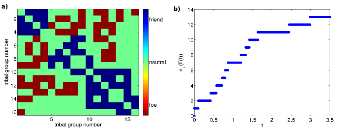
Figure 9: The PNG dataset from [37]. In frame (a), we are plotting the interaction matrix amongst the 16 tribes. Blue pixels correspond to entries in ${{\Gamma}_{+}}$, red to entries in ${{\Gamma}_{-}}$. In frame (b), we plot $n_{+}({\Gamma}(t))$ as a function of $t$; we know that this is positive for all $t>0$, since $c({{\Gamma}_{+}})>0$, and we see that it increases to its maximum value around $t=3.0$.

For the Slashdot Zoo data set, we concentrated on the component of the Slashdot database that is friendly to CmdrTaco, the founder of the site and user number 1. More specifically, we considered only those users for which there existed a “friendly path” from that user to CmdrTaco. This subset was, not surprisingly, the largest connected component of the full network, and contains 23,514 users. We then considered the subgraph of these 23,514 users to itself, and this is what we define ${\Gamma}$ to be. This graph contains 415,118 positive edges and 117,024 negative edges, and we computed components. By definition, $c({{\Gamma}_{+}})=1$, and we compute that $c({{\Gamma}_{-}})=$ 10,327, giving ${\Gamma}$ a flexibility index of 13,187. This is, admittedly, a one-off calculation, but we conjecture that data from social networks will show this pattern, that even amongst a group of “friends”, or common “fans” of a particular user, there will be a large number of instabilities in exactly this manner.

References

- [1] Slashdot website. url http://www.slashdot.org/.
- [2] J.A. Acebrón, L.L. Bonilla, C.J.P. Vicente, F. Ritort, and R. Spigler. The Kuramoto model: A simple paradigm for synchronization phenomena. Reviews of modern physics, 77(1):137, 2005.
- [3] Francesco Brenti. Log-concave and unimodal sequences in algebra, combinatorics, and geometry: an update. In Jerusalem combinatorics ’93, volume 178 of Contemp. Math., pages 71–89. Amer. Math. Soc., Providence, RI, 1994.
- [4] Jared C. Bronski, Lee DeVille, and Moon Jip Park. Fully synchronous solutions and the synchronization phase transition for the finite-N Kuramoto model. Chaos, 22(033133), 2012.
- [5] P. R. Bryant. Graph theory applied to electrical networks. In Graph Theory and Theoretical Physics, pages 111–137. Academic Press, London, 1967.
- [6] Seth Chaiken. A combinatorial proof of the all minors matrix tree theorem. SIAM J. Algebraic Discrete Methods, 3(3):319–329, 1982.
- [7] F.R.K. Chung. Spectral Graph Theory (CBMS Regional Conference Series in Mathematics, No. 92). American Mathematical Society, 1997.
- [8] C. R. Crawford. A stable generalized eigenvalue problem. SIAM J. Numer. Anal., 13(6):854–860, 1976.
- [9] C. R. Crawford. Errata: “A stable generalized eigenvalue problem” (SIAM J. Numer. Anal. 13 (1976), n0. 6, 854–860). SIAM J. Numer. Anal., 15(5):1070, 1978.
- [10] D.M. Cvetkovic, M. Doob, and H. Sachs. Spectra of graphs: Theory and application, volume 413. Academic press New York, 1980.
- [11] Lee DeVille. Transitions amongst synchronous solutions in the stochastic kuramoto model. Nonlinearity, 25(5):1473, 2012.
- [12] Chris Godsil and Gordon Royle. Algebraic graph theory, volume 207 of Graduate Texts in Mathematics. Springer-Verlag, New York, 2001.
- [13] L. Goeritz. Knoten und quadratische formen. Mathematische Zeitschrift, 36(1):647–654, 1933.
- [14] C.M. Gordon and RA Litherland. On the signature of a link. Inventiones mathematicae, 47(1):53–69, 1978.
- [15] Werner H. Greub. Linear algebra. Second edition. Die Grundlehren der mathematischen Wissenschaften, Bd. 97. Academic Press Inc., Publishers, New York, 1963.
- [16] Per Hage and Frank Harary. Structural models in anthropology, volume 46 of Cambridge Studies in Social Anthropology. Cambridge University Press, Cambridge, 1983. With a foreword by J. A. Barnes.
- [17] Y. Hatano and M. Mesbahi. Agreement over random networks. Automatic Control, IEEE Transactions on, 50(11):1867 – 1872, nov. 2005.
- [18] YaoPing Hou. Bounds for the least laplacian eigenvalue of a signed graph. Acta Mathematica Sinica, 21:955–960, 2005.
- [19] June Huh. Milnor numbers of projective hypersurfaces and the chromatic polynomial of graphs. J. Amer. Math. Soc, 25(3):907–927, 2012.
- [20] June Huh and Eric Katz. Log-concavity of characteristic polynomials and the Bergman fan of matroids. Math. Ann., 354(3):1103–1116, 2012.
- [21] Vaughan F. R. Jones. A polynomial invariant for knots via von Neumann algebras. Bull. Amer. Math. Soc. (N.S.), 12(1):103–111, 1985.
- [22] Akshay Kashyap, Tamer Başar, and R. Srikant. Quantized consensus. Automatica, 43(7):1192 – 1203, 2007.
- [23] Tosio Kato. Perturbation theory for linear operators. Springer-Verlag, Berlin, second edition, 1976. Grundlehren der Mathematischen Wissenschaften, Band 132.
- [24] Louis H. Kauffman. State models and the Jones polynomial. Topology, 26(3):395–407, 1987.
- [25] Louis H. Kauffman. A Tutte polynomial for signed graphs. Discrete Appl. Math., 25(1-2):105–127, 1989. Combinatorics and complexity (Chicago, IL, 1987).
- [26] G. Kirchhoff. Uber die aufiiisung der gleichungen, auf welche man bei der untersuchung der unearen verteilung galvanischerstriime gefuhrt wird. Ann. Physik Chemie, 72:497–508, 1847.
- [27] G. Kirchhoff (Trans. J.B. O’Toole). On the solution of the equations obtained from the investigation of the linear distribution of galvanic currents. IRE Trans. Circuit Theory, 5:4–8, 1958.
- [28] Jérôme Kunegis, Stephan Schmidt, Andreas Lommatzsch, and Jürgen Lerner. Spectral analysis of signed graphs for clustering, prediction and visualization. In Proc. SIAM Int. Conf. on Data Mining, pages 559–570, 2010.
- [29] Y. Kuramoto. Chemical oscillations, waves, and turbulence, volume 19 of Springer Series in Synergetics. Springer-Verlag, Berlin, 1984.
- [30] Y. Kuramoto. Collective synchronization of pulse-coupled oscillators and excitable units. Physica D, 50(1):15–30, May 1991.
- [31] Renato E. Mirollo and Steven H. Strogatz. Synchronization of pulse-coupled biological oscillators. SIAM J. Appl. Math., 50(6):1645–1662, 1990.
- [32] Renato E. Mirollo and Steven H. Strogatz. The spectrum of the locked state for the Kuramoto model of coupled oscillators. Phys. D, 205(1-4):249–266, 2005.
- [33] Renato E. Mirollo and Steven H. Strogatz. The spectrum of the locked state for the Kuramoto model of coupled oscillators. Phys. D, 205(1-4):249–266, 2005.
- [34] James R. Munkres. Elements of algebraic topology. Addison-Wesley Publishing Company, Menlo Park, CA, 1984.
- [35] R. Olfati-Saber, J.A. Fax, and R.M. Murray. Consensus and cooperation in networked multi-agent systems. Proceedings of the IEEE, 95(1):215 –233, jan. 2007.
- [36] Beresford N. Parlett. Symmetric matrix pencils. In Proceedings of the International Symposium on Computational Mathematics (Matsuyama, 1990), volume 38, pages 373–385, 1991.
- [37] K. E. Read. Cultures of the central highlands, new guinea. Southwestern Journal of Anthropology, 10(1):pp. 1–43, 1954.
- [38] Shigeru Shinomoto and Yoshiki Kuramoto. Phase transitions in active rotator systems. Progress of Theoretical Physics, 75(5):1105–1110, 1986.
- [39] Richard P. Stanley. Log-concave and unimodal sequences in algebra, combinatorics, and geometry. In Graph theory and its applications: East and West (Jinan, 1986), volume 576 of Ann. New York Acad. Sci., pages 500–535. New York Acad. Sci., New York, 1989.
- [40] Steven H. Strogatz. From Kuramoto to Crawford: exploring the onset of synchronization in populations of coupled oscillators. Phys. D, 143(1-4):1–20, 2000. Bifurcations, patterns and symmetry.
- [41] W. T. Tutte. Graph theory, volume 21 of Encyclopedia of Mathematics and its Applications. Cambridge University Press, Cambridge, 2001. With a foreword by Crispin St. J. A. Nash-Williams, Reprint of the 1984 original.
- [42] Mark Verwoerd and Oliver Mason. Global phase-locking in finite populations of phase-coupled oscillators. SIAM J. Appl. Dyn. Syst., 7(1):134–160, 2008.
- [43] Mark Verwoerd and Oliver Mason. On computing the critical coupling coefficient for the Kuramoto model on a complete bipartite graph. SIAM J. Appl. Dyn. Syst., 8(1):417–453, 2009.
- [44] L. Xiao and S. Boyd. Fast linear iterations for distributed averaging. Systems & Control Letters, 53(1):65–78, 2004.
- [45] Lin Xiao, Stephen Boyd, and Seung-Jean Kim. Distributed average consensus with least-mean-square deviation. Journal of Parallel and Distributed Computing, 67(1):33 – 46, 2007.
- [46] T. Zaslavsky. Bibliography of signed and gain graphs. The Electronic Journal of Combinatorics, 1000:DS8–Sep, 2002.
- [47] Thomas Zaslavsky. Signed graph coloring. Discrete Mathematics, 39(2):215 – 228, 1982.
- [48] Thomas Zaslavsky. Signed graphs. Discrete Applied Mathematics, 4(1):47 – 74, 1982.
- [49] Thomas Zaslavsky. Strong Tutte functions of matroids and graphs. Trans. Amer. Math. Soc., 334(1):317–347, 1992.