Biophysics software for interdisciplinary education and research

Abstract

Biophysics is a subject that is spread over many disciplines and transcends the skills and knowledge of the individual student. This makes it challenging both to teach and to learn. Educational materials are described to aid in teaching undergraduates biophysics in an interdisciplinary manner. Projects have been devised on topics that range from x-ray diffraction to the Hodgkin Huxley equations. They are team-based and encourage collaboration. The projects make extensive use of software written in Python/Scipy which can be modified to explore a large range of possible phenomena. The software can also be used in lectures and in the teaching of more traditional biophysics courses.

1 Introduction

Many of the most active and productive areas in science are rapidly becoming highly interdisciplinary, with teams of researchers from diverse fields discovering new phenomena and creating new technology that would be impossible within the confines of a single discipline. The range of knowledge of an single individual necessary to create, for example, rapid gene sequencing technology is beyond the capacity of even the most gifted polymaths. Current research often involves researchers taking place in separate areas It is now necessary to have work on different aspects of a project, that require completely different expertises, and then to combine these efforts to achieve the final result.

Education has had a hard time keeping pace with the rapidly changing face of technological and scientific advancement, with the majority of learning taking place within a single field, and not addressing the important issues involved with collaboration across very different fields. In this paper I will describe the software and learning tools that have been developed to create an interdisciplinary learning environment. It attempts to teach students from different disciplines how to collaborate in a way that mimics the real challenges faced today in biophysics research.

The course spanned one quarter, that is ten weeks, plus student presentations, and involved approximately four hours of lectures and typically three hours of discussion sections per week. The number of students in the course ranged from 12 to 21.

Learning in this course focuses on several weekly projects that are studied by interdisciplinary teams for students. Each team is normally composed of three students from a wide range of backgrounds and majors. For example, a physics, biochemistry, and biomolecular engineering major. The projects use software written in SciPy [1, 2], to serve multiple functions: sometimes to perform simulations that act as artificial experimental input, sometimes used to analyze data, and to gain theoretical and intuitive understanding of biophysical processes in a way that requires active learning. One student, typically, is responsible for a particular area, such as computer coding, mathematical and physical analysis, or biological and biochemical understanding. The problems are designed to promote interaction between the different majors, to teach them about interdisciplinary collaboration and allow them to exchange knowledge and approaches to scientific problems.

This course has now been taught three times, and an evaluation of the efficacy of this approach including the results of student assessments will be addressed in a future publication. This work will focus specifically on the tools used. Not only is this useful to other educators interested in using these tools, but also provides a wealth of useful simulations that can be used on their own, and can be useful in both teaching and in research.

The material has been modified and enlarged as more experience on its efficacy has been obtained. Because the author is a physicist and has had little experience teaching the life sciences, an exceptionally talented biochemistry major, Michelle V. Mai, who had previously taken this course, was recruited to help in amending and designing questions that would be most beneficial to the biology and biochemistry undergraduates. The course has been highly successful and has had a major impact on many of the students who have taken it. It has often influenced their career choice, either towards biophysics, or software development, and has obtained consistently high evaluations from the students. The author believes that it is therefore worthwhile disseminating the tools used in this course and describing how it was taught.

2 Uses of material

The main purpose of this paper is to introduce instructors to the biophysics material that I have developed. The material develops a range of skills, in understanding biological processes, physical laws, mathematical analysis, software development, and interdisciplinary collaboration. The material can be used in many different ways as I now describe.

The easiest use of this material is in lecture demonstrations. A variety of physical and biophysical processes can be demonstrated and the relatively simple python source code allows for flexibility in making changes, even during lecture. For this purpose, the audience can be undergraduates at all levels, and graduate students. It was found to be very useful to derive theoretical predictions and then test these numerically in real time. Often it was found that these simulations made theoretical discussion much more tangible and led to a lot of questions and interaction during lectures.

It can be used to supplement already existing biophysics courses with material that students can use, either as homework, or as special projects. The courses do not have to be interdisciplinary in composition and can be composed of physics majors, but this will require modification of the problems. The material is often presented with incomplete software, allowing students to fill in important steps to complete the code. Instead the software can be supplied to students in a completely working state. In that way, the simulations become more like experiments, and potentially even lower division students with a small amount of computer experience can benefit from some of these projects.

Finally it can be used as I have, as the basis for a new biophysics course at the upper division or graduate level.

3 Type of projects

The projects spanned a wide range of problems in biophysics.

Most projects were due in a week, but several were two week projects. Students would typically submit several projects every week. These would often require the submission of a progress report at the end of a week to ensure their timely completion. Some of the projects were tailored to the research interests of students who were currently taking the course. For example, the “Distribution of ATP and mitochondria in axons” is a research topic of current interest to William Saxton on the biology faculty at UCSC, and a team of students had meetings with him to determine how to most usefully model this process.

Most of these have one or more SciPy programs associated with them, but some were analytical, and one involved other software (Foldit). Aside from the software component, there were physical and biological aspects that needed to be addressed by the students.

In order to be teachable in a space of ten weeks, there were three common physical and mathematical themes that ran through the course that enabled the students to build on what they had learned: Fourier Transforms, diffusion, and molecular simulations.

The projects are described below in nearly chronological order, so as to explain in more detail how a fairly substantial territory was covered in a way that was accessible to the students with very diverse backgrounds.

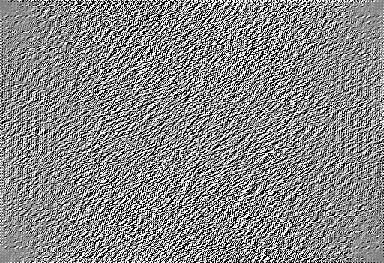
Figure 1: An image that needs to be decoded. The intensities are related to the Fourier transform for the original image. This introduces the idea needed in x-ray diffraction that inverting Fourier transform data can give you a lot of structural information.

(a)

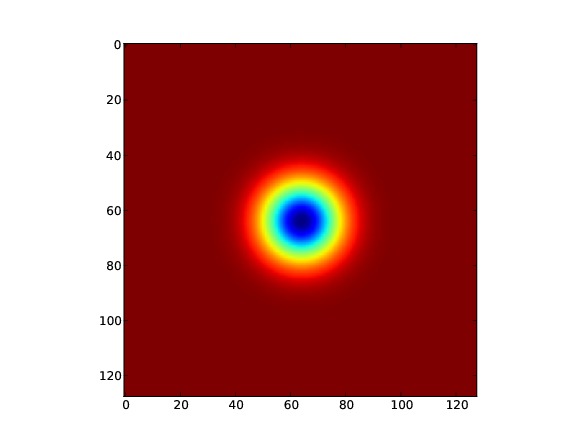
(b)

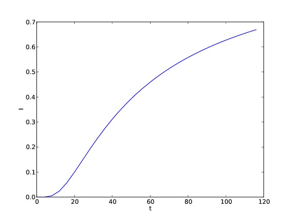
Figure 2: A simulation of FRAP. An area a circular area is photobleached and a simulation of the evolution of density is displayed. (a) A snapshot of the intensity during the simulation. (b) A plot of the intensity as a function of time at the center of the circle.

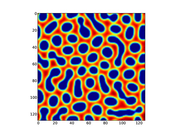
Figure 3: A simulation of FRAP. An area a circular area is photobleached and simulation of the evolution of density is displayed. (a) A snapshot of the intensity during the simulation. (b) A plot of the intensity as a function of time at the center of the circle.

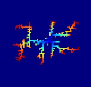
Figure 4: A simulation of Diffusion Limited Aggregation which is important in understanding many physical processes including the morphology of bacterial colonies.

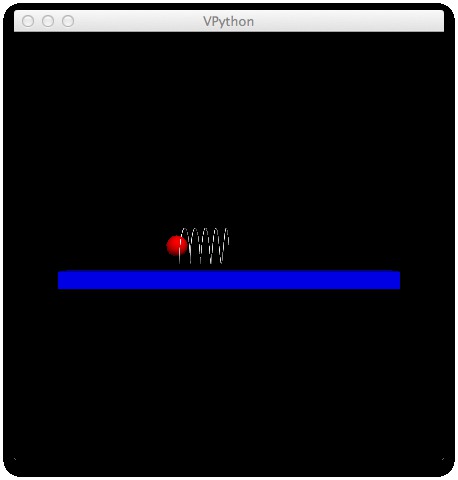
Figure 5: A snapshot of a simulation of the Langevin equation for a particle in a highly viscous fluid coupled to a spring. This is the same mathematically as the model used to understand noise in optical traps. The graphics was easily implemented using visual python [3].

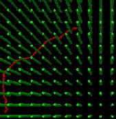
Figure 6: A snapshot of a simulation of electrophoresis of DNA going through an array of nanopillars shown using visual python [3].

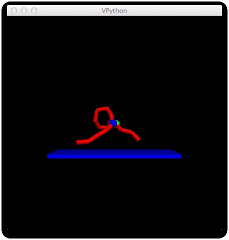
Figure 7: A snapshot of a simulation of a molecule with two metastable internal states, to study Single Molecule Force Spectroscopy.

3.1 Scope of projects

The following goes through a synopsis of the material taught using the materials discussed here. The plots and simulations shown are a small subset of the ones available to the students. They are shown as they would appear to them.

• The course started out with setting up SciPy on their individuals computers. They learned the basics of input/output by reading in image files that contained coded images that could be decoded by several operations including the two dimensional inverse Fourier Transform. Fig. 1 shows the initial image that needs to be decoded. The real part of the Fourier transform has been processed in a way that allows for a reasonable quality when inverted, despite the small number of bits used to encode each point. When decoded it leads to a picture that is recognizable to a life science student.

• The next set of projects involves x-ray diffraction, and tomography, both of which use Fourier Transforms. In two of the projects, students were given fake computer generated data, (tomographic or diffraction) and had to invert it to get the underlying structure. The goal to find a structure mimics research more closely than book problems that do not have such a tangible outcome.

• Diffusion is introduced. The differential equations describing this process are quite familiar to physics majors, but the underlying connection with the physical process of random motion is not usually explained. Computer projects introduced two methods for understanding diffusion. One is from the differential equation perspective, and the other using random walks. By going through several of these projects, that contain a lot of visualization, this connection becomes far clearer, and also introduces random molecular motion to students. There is a plethora of biological applications of diffusive processes and this also helps maintain interest for students in the biological disciplines. One important technique, Fluorescence recovery after photobleaching [4] (FRAP), is nicely illustrated by computer simulation, (Fig. 2). A region is photobleached and molecules diffuse resulting in a changing fluorescence intensity. This project gets students to think about how a combination of scaling and simulations can give quantitative predictions for experiments. These techniques are rarely taught but can be appreciated, without the need for sophisticated mathematics.

• Most other problems could be leveraged from knowledge of these three areas. In this week, various aspects of morphogenesis were discussed, and patterns such as those produced by reaction-diffusion equations are now understandable by modifying the diffusion code to include more than one kind of diffuser, and nonlinear interactions. The model introduced by Turing giving rise to patterns on the skin of animals can be modeled numerically (Fig. 3) and give rise to a variety of different morphologies such as stripes and spots. These can be understood by adjusting parameters in the models and the boundary conditions. The most important lesson that comes out studying this is how complexity comes out of simple physical processes. Biology students were able to investigate to what extent these principles are applicable to real problems. Other problems with biological relevance, such as dendritic growth and Diffusion Limited Aggregation [5] (DLA) can now be taught, and simulations of these can be modified by students to explore their behavior and relation to biology. For example there has been much experimental work relating DLA (Fig. 4) to the morphology of bacterial colonies [6, 7]. Students not only learn how to write such simulations but by collaborating can critically assess evidence supporting this mechanism in experimental systems.

• Instead of using differential equations to understand diffusion, a more basic approach can be taken that uses the underlying random motion. This starts the learner down the path of studying dynamics of particles in liquids, taking into account their thermal motion. To understand such problems, correlations and power spectra are crucial, and this also relates back to Fourier Transforms. Particles in optical trap provide an excellent illustration of these principles, as well as being closely related to a very active area of biophysical research. A simple example of this that can be easily simulated is a particle tethered by a spring in a viscous liquid acted on by random thermal motion (Fig. 5). This is perhaps the most difficult part of the course to understand from a mathematical perspective, and the projects employ simulations of these systems, to obtain data as if they were experiments. By analyzing these experiments by means of Fourier Transform and correlation functions [8], students appeared to grasp the underlying physics quite well. This is also related to the more difficult problem of bacterial chemotaxis, for example, how bacteria move to regions of higher glucose concentration despite being too small to be able to effectively detect chemical gradients. Many of the same ideas can be applied to this interesting biological problem.

  

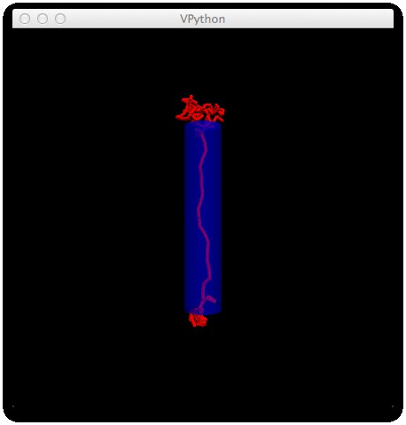
  Figure 8: A snapshot of a simulation of a macromolecule translocating through pore in a membrane. It is visualized using visual python [3].

  

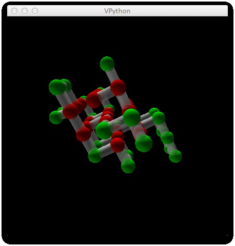
  Figure 9: A snapshot of the folding of a protein on a lattice, using the HP model, and Monte Carlo and simulated annealing.

  

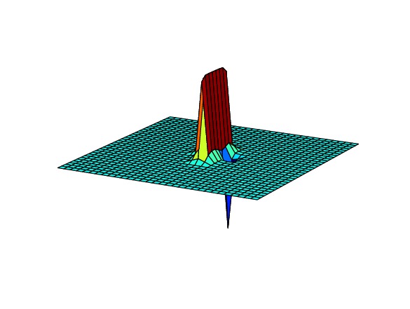
  Figure 10: The potential around a collection of charges in two dimensions according to the non-linear Poisson Boltzmann equation.

• The above systems contain only a few degrees of freedom. The next logical step is to consider many degrees of freedom, such as the dynamics of macromolecules. There are a large number of biophysical systems that can be readily investigated by simulations and are highly educational. The electrophoresis of DNA can be described by simulating a string going through a network of rigid obstacles. The dynamics show semi-periodic behavior [9], that can be easily seen by simulations visualized in three dimensions using visual python [3], see Fig. 6. This leads to an understanding of pulsed field electrophoresis, which has been instrumental in separation of very long DNA that cannot be separated by the constant field case. Using a modification of this code, it is possible to understand the force versus displacement in stretching a DNA chain which is accessible experimentally using optical traps. More generally, recent experiments stretching of macromolecules, such as RNA, that have complex internal states, leads to a much increased understanding of their structure. This technique, Single Molecule Force Spectroscopy [10], is also possible to understand directly by simulations (Fig. 7. In this case a molecule has two groups that have an attractive interaction so that when it is pulled by its ends, it has metastable behavior giving rise to hysteresis loops. Conversely, if one is given experimental data on the stochastic transitions between multiple internal states, analyzing the details of these transitions gives much useful information about the nature of the molecule. This is also examined in another project. Other projects have also been developed, including the translocation of linear macromolecules through a nanopore (Fig. 8), which is an active area of research at UC Santa Cruz and elsewhere [11].

  (a)

  (b)

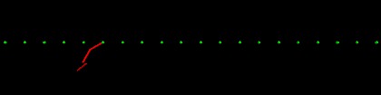
  Figure 11: Two snapshots (a) and (b) of a minimal simulation of myosin V on actin capturing the essential physics of motor motion. The motion is similar to hand-over-hand motion used on “monkey bars”.

• One of the most widely studied class of macromolecules are proteins. Because of their emphasis in biophysics, and their fascinating properties, a number of projects were developed. A number of important physical phenomena are studied here, the coil-globule transition, the helix-coil transition, and the determination of the folded state of a protein. This problem of “protein folding” is studied for simplified models such as the so-called “HP” model of Dill and Chan [12], see Fig. 9. This is a good model to simulate using Monte Carlo methods, and leads to an understanding of the energy landscape of this problem. The problem is still interesting with further simplification, studying it in two dimensions. A powerful variations of Monte-Carlo, such as parallel tempering is also studied. To speed up these simulations, C code is embedded using “weave” [13], which introduces some of the more computer oriented students to C programming. A phenomenal piece of software that folds proteins called “Foldit” which is freely available [14] is excellent for elucidating many of the subtle interactions seen in proteins. It has been written in the form of a computer game and has been very popular and players have produced some excellent structures [15].

• Some of the more subtle features of macromolecular interaction are electrostatic and these can be approximately described in some cases by the non-linear Poisson Boltzmann equation [16]. Students learn how to solve this equation, whose solution closely resembles earlier work they did on morphogenesis (Fig. 10). There are also two projects involving biological motors. The first is a minimal model of myosin V [17] that can be understood by a simulation incorporating chain stiffness, binding and unbinding from a linear array of sites. Students can change parameters in the model, such as bounding angles, and chain stiffness, to see what motors work best. Two snapshots from such a simulation are given in (Fig. 11). Different teams design motors with different parameters and run a race to see which motor works best. Another problem that is currently being studied at UC Santa Cruz [18, 19] is that of cytoplasmic streaming in drosophila oocytes. This can be modeled by a variation of the DNA simulations done in week 6. This leads to an interesting set of behavior such as a breaking of chiral symmetry, and collective organization of microtubules to advect fluid chaotically through the cell. Fig. 12 shows a snapshot of a microtubule moving as a rotating helix due to the action of kinesin motors walking upwards along its surface.

  

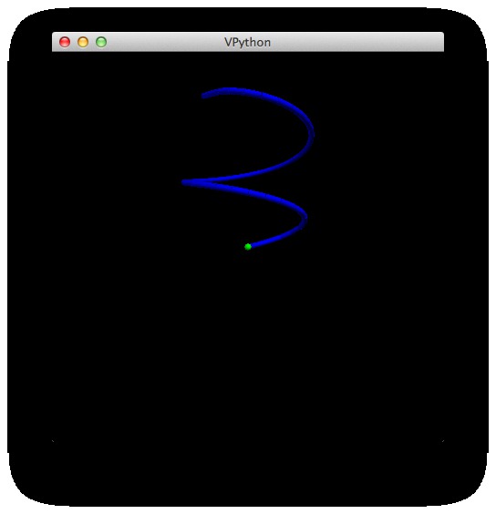
  Figure 12: A snapshot of a microtubule moving inside a Drosophila oocyte. The rotating helical motion is a consequence of the force generated by kinesin motors walking along its backbone.

  

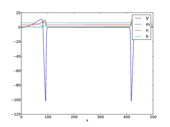
  Figure 13: A snapshot of a simulation of action potentials travelling down an axon as described by the Hodgkin Huxley equations.

• The course ends with an introduction to biophysics of the neuron. The Hodgkin Huxley equations [20] are modelled to explain how action potentials are generated and propagate. The propagation of a spike is shown in Fig. 13. Complementary to this is the high level organization of neural networks. Using code similar in spirit to that used earlier to study the Helix Coil transition, the mechanism for associative memory proposed by Hopfield is implemented.

3.2 List of projects

Here is the list of projects offered in this course.

1. Introduction

   1. Using SciPy and Inverse Fourier Transforming Images

2. Imaging techniques

   1. Reconstructing a 2D Structure From X-ray Data

   2. Introduction to Tomography

   3. Analytic methods in diffraction

   4. Introduction to NMR (Two week project)

   5. Image processing

3. Diffusion

   1. 1 dimension

      1. Binomial Distribution, Diffusion, Central Limit Theorem

      2. Mean time to capture by diffusion in 1 dimension

      3. Steady state solution of the diffusion eq in 1 dimension

      4. Comparing numerical and analytic solutions to the diffusion eq.

   2. 3 dimensions

      1. Probability of capture by a spherical absorber by diffusion

      2. Diffusion to a disk-like absorber

      3. Diffusion through many circular apertures in a planar barrier

   3. Using FRAP to determine a diffusion coefficient

   4. Kirby Bauer Antibiotic Testing

   5. Distribution of ATP and mitochondria in axons

4. Morphogenesis

   1. Reaction Diffusion and Biological Patterns

   2. Flow lines in Murray’s model of pattern formation

   3. Morphogenesis by the mechanism of Diffusion Limited Aggregation

   4. Origins of dendritic growth

5. Dynamics with thermal motion

   1. Correlation functions and power spectra

   2. Brownian motion in an optical trap

   3. Brownian motion of a free particle

   4. Modeling bacterial chemotaxis

6. Dynamics of Macromolecules

   1. Motion of DNA during gel electrophoresis

   2. Force on ends of DNA chain

   3. Translocation of a linear macromolecule through a nanopore

   4. Determining molecular states from force data

   5. Hysteresis in Single Molecule Force Spectroscopy

   6. Force on a freely jointed chain

7. Understanding Protein interactions and folding

   1. Foldit

   2. Coil Globule transition

   3. Helix Coil transition

   4. 2D HP model

   5. Folding time for the HP model

   6. Using Parallel Tempering to fold a protein

   7. Effect of charges in solution

8. Motor proteins

   1. Myosin simulation race

   2. Cytoplasmic streaming in drosophila oocytes

9. Membrane potentials and the Hodgkin Huxley Equations

10. The Hopfield Model

4 Required student level of knowledge

At the beginning of the quarter, teams of three were formed, with the goal to have enough diversity in knowledge in each team so as to effectively tackle the projects assigned.

4.1 Software

For each team, there was normally one student who had some degree of exposure to programming. The physics majors are required to take introductory programming and sometimes students from other majors, particularly in the engineering disciplines were quite knowledgeable. The software was provided to the students, in variety of states; sometimes as fully functioning code, other times with a few lines that needed to be filled-in, and rarely where more extensive modifications were needed to be made.

The software platform was chosen to follow a middle ground between two very different pedagogical uses of computers in education. The first scenario is exemplified by numerical methods courses. There, simulation code is developed commonly in a highly efficient language, such as C, C++, Fortran, or Java, to learn how to do state-of-the-art simulations using a variety of numerical techniques, such as Monte Carlo, or Molecular Dynamics simulations. Such courses require students that typically have a reasonably advanced knowledge of Applied Mathematics and the ability to code at an intermediate level in one of the above languages. The other scenario is to teach a course that already has a graphical user interface (GUI) programmed in, and students navigate the interface to make changes in parameters, or have a restricted choice in how the software functions. Excellent biophysics software of that type has been recently developed [21] and this approach has been pioneered more than two decades ago [22].

The software in this course is at neither of these two extremes. It is recognized that the majority of physics and engineering majors have not had a rigorous numerical methods course, but at the same time do typically have a fair degree of programming proficiency. At the same time, code even with the most flexible GUI interface, cannot come close to the flexibility attainable using source code. It is very hard to have the flexibility to allow students to answer the large number of questions that come to mind, when exploring a new biophysical system. These are the kind of questions that one would expect to answer when doing research, and is indeed why SciPy has been so popular with the research community. Scipy code is being extensively developed for use in teaching by others as well [23]. It allows fairly complex problems to be addressed with a minimum of programming overhead, and also has advanced graphics capabilities allowing data to be displayed in a variety of different ways. Visual Python [3] was also used. It displays excellent three dimensional visualization of systems, such as macromolecules, with a minimum of extra code.

That being said, there was still a fair amount of learning that was necessary to become proficient in the programming tools that were used and the course was designed to make this possible for the students to achieve. The learning of this skill was often listed as a major benefit of having taken this course.

At the beginning of the course, the code was at a fairly basic level, and eschewed the use of classes or other high level constructs that might be unfamiliar to many of the students. As the quarter progressed, the programs became more advanced and some C-code was integrated into the Python source through “weave” [13] to increase its efficiency.

In general, the teams handled the software component of the projects very well. In most cases students only needed to change parameters in the code, and the students were able to follow the structure of the code sufficiently well to be able to make these changes. In fact, quite a few of the biology and biochemistry students were able to pick up enough programming to do this on their own. Some of them ended up becoming quite proficient at coding.

There was quite a lot of choice students were given in projects that they would work on. Therefore the teams less interested in software development would choose projects the did not require much programming. On the other hand, some students were very interested in this aspect, and occasionally produced very impressive modifications or wrote their own code, for example, in Java. This flexibility in coding emphasis led to more enthusiasm among the students, who could often do work of an unexpectedly advanced nature.

The most difficult part of this course was the initial installation of SciPy and Visual Python on students’ own computers. These are both complex pieces of software undergoing constant development. The operating systems that worked best were Linux or Windows based. Mac computers have been the most problematic. Some students were unable or unwilling to upgrade their mac operating systems which made it much harder for them to get a working version of SciPy. The latest releases of SciPy from Enthought [24], which has a free academic license, worked well. However there are still major issues with Visual Python. Some of these are problems with graphics cards, and with some incompatibility of libraries between Visual Python and the standard ones that are installed by Linux, and conflicts between Enthought and Visual Python on a mac. Still, the vast majority of students found a way of getting a working system to enable them to modify and run the code for this course. The author has been able to get the software to run on versions of all three operating systems, but because of the nature of software, this is a constantly changing target.

4.2 Knowledge of Biology and Biochemistry

There was a significant fraction of students in this class that were not from a physics background and primarily focused on biology or biochemistry.

The course is focused on biology and therefore the problems that need to be solved were at a level that requires a fair amount of biological sophistication. An attempt was made, from the first assignment, to ensure that these students’ contribution was necessary for a project’s successful completion, even if a particular problem was mostly one involving mathematics. For example, the first assignment required a small modification in code in order to decode the Fourier Transform of an image. The object was to determined what a set of images represents as shown in Fig. 1. The last time the course was taught, the images were chosen to come from biology or biochemistry, and it would have been quite hard for physics majors to correctly identify them. This kind of interaction between the different disciplines from the outset, was found to greatly improve the cohesion of the teams and was later evident in the increased degree of collaboration between members.

Aside from software or physics components, there were usually questions that required an upper division knowledge of biology or chemistry. These questions were of a somewhat different character than you typically find in biology courses. They often were more open-ended and allowed students with different backgrounds to focus on different aspects of a problem.

There was an effort made to come up with problems that required a person familiar with biological sciences to understand. Often it was necessary for teams to understand one or more biophysics articles in order to undertake a project. For example the project to understand Fluorescence Recovery After Photobleaching (FRAP), which is a common biophysical technique, is not taught to physics students. References were given to papers that would be much more comprehensible to biology or biochemistry students, who could then translate the work into something a physics major could understand. Problems often asked students to use their knowledge of biology to come up with situations where a physical process, for example absorption of diffusers, would be relevant, and to what extent such physical consideration would be applicable.

Because there was a fair amount of choice in projects, teams could choose problems more in line with their individual interests. There were problems that were popular with neuroscience students for example, such as studying MRI. Or there were specific problems, for example, the translocation of a chain through a nanopore, or the Poisson Boltzmann equation, that were of interest to students that had done laboratory research in that area. These students could use their expertise to collaborate more effectively with team members that were more software or mathematically oriented, and this would be mutually beneficial to the whole team.

5 Course materials

The website for the course is http://physweb.ucsc.edu/drupal/courses/physics-180-spring-2012. This contains the projects used in this course and other information such as links to the material used in the lectures and projects. The code provided to the students is, in some cases, deliberately incomplete. Instructors can email the author (josh@ucsc.edu) to obtain a full set of python source code and data files.

References

- [1] http://scipy.org
- [2] Oliphant T E 2007 Computing in Science and Engineering 9 10-20
- [3] http://vpython.org
- [4] Axelrod D, Koppel, D, Schlessinger, J, Elso, E and Webb W 1976 Biophysical Journal 16 1055–69
- [5] Witten T A and Sander L M, 1981 Phys. Rev. Lett. 47, 1400-3
- [6] Matsuyama T and Matsushita M, 1993 Critical Reviews in Microbiology 19 117-135
- [7] Kozlovsky Y Cohen I Golding I and Ben-Jacob E, 1999 Phys. Rev. E. 59 7025-7035
- [8] Reif F 1965 “Fundamentals of statistical and thermal physics” McGraw-Hill Section 15.8
- [9] J.M. Deutsch, 1988 Science 240 922-924
- [10] Michael T W Garciá-Garciá C. and Block S M 2008 Current Opinion in Chemical Biology 12 640–646
- [11] Winters-Hilt S Vercoutere W DeGuzman VS Deamer D Akeson M and Haussler D 2003 Biophys J. 84 967-76
- [12] Lau K F, and Dill K A 1990 Proc. Natl. Acad. Sci. 87 638-642
- [13] http://www.scipy.org/Weave
- [14] http://fold.it/portal/
- [15] Khatib F Dimaio F Cooper S Kazmierczyk M Gilski M Krzywda S Zabranska, H Pichova I. et al. 2011 Nature Structural & Molecular Biology 18 1175-1177
- [16] “Soft-Matter Characterization, Vol 2” 2008 Eds. Borsali R and Pecora R, Springer P. 295
- [17] Dunn A R and Spudich J A 2007 14 Nature Struct. & Mol. Biol. 246-48
- [18] Serbus L R Cha, B J Theurkauf W E and Saxton W M 2005 Development 132 3743-3752
- [19] Deutsch J M Brunner M E Saxton W M 2011 http://arxiv.org/abs/1101.2225
- [20] Hodgkin A L and Huxley A F 1952 J. Physiol. 117 500-44
- [21] Tinker R and Xie Q 2008 Computing in Science and Engineering 10 24-27
- [22] Weiss T F Trevisan G Doering E B Shah D M Huang D, and Berkenblit S I 1992 J Sci. Ed. and Tech. 1 259-274
- [23] Myers C R and Sethna J P 2007 Computing in Science and Engineering 9 75
- [24] http://enthought.com