Domain-of-Attraction Estimation for Uncertain Non-polynomial Systems*

Abstract

In this paper, we consider the problem of computing estimates of the domain-of-attraction for non-polynomial systems. A polynomial approximation technique, based on multivariate polynomial interpolation and error analysis for remaining functions, is applied to compute an uncertain polynomial system, whose set of trajectories contains that of the original non-polynomial system. Experiments on the benchmark non-polynomial systems show that our approach gives better estimates of the domain-of-attraction.

1 Introduction

Stability for nonlinear control systems plays an important role in control system analysis and design. It will be very useful to know the domain of attraction (DOA) of an equilibrium point, however, this region is usually difficult to find and represent explicitly. Therefore, looking for underestimates of the DOA with simple shapes has been a fundamental issue in control system analysis since a long time. Among all the methods, those based on Lyapunov functions are dominant in literature [3, 4, 6, 7, 8, 11, 16, 19, 22, 20, 10, 21, 15]. These methods not only yield a Lyapunov function as a stability certificate, but also the corresponding sublevel sets as estimates of the DOA.

For polynomial systems, many well-established techniques ([6, 8, 7, 11, 16, 19, 22, 20, 10, 21, 15]) are available for computing estimates of DOAs. In [19], a method based on SOS decomposition was presented to find provable DOAs and attractive invariant sets for nonlinear polynomial systems. For odd polynomial systems, [6] employed an LMI-based method to compute the optimal quadratic Lyapunov function for maximizing the volume of the largest estimate of the DOA. To obtain estimates of DOAs of uncertain polynomial systems, the authors of [8] used discretization (in time) to flow invariant sets backwards along the flow of the vector field. In [16], quantifier elimination (QE) method via QEPCAD was also applied to find Lyapunov functions for estimating the DOA. However, these methods cannot be applied directly in practice since most real systems are non-polynomial systems, i.e, their vector fields contain non-polynomial terms. For this kind of systems, only a few approaches have been proposed to deal with the DOA analysis. In [3, 4, 5], the author proposed an LMI technique through Taylor expansions as substitution for non-polynomial terms, and this technique can be generalized to compute estimates of DOAs for uncertain non-polynomial systems. In [23], an interval arithmetic approach was proposed. Recently, [18, 17] suggested a new method, based on quadratic Lyapunov function and the theorem of Ehlich and Zeller.

In this paper, we will consider the problem of stability region analysis of uncertain non-polynomial systems. Through multivariate polynomial interpolation together with the interpolation error analysis, we substitute a non-polynomial system as an uncertain polynomial system, whose set of trajectories contains that of the original non-polynomial system. By computing estimates of the DOA for the resulted uncertain polynomial system, we obtain estimates of the DOA for the original non-polynomial system. Our method is also applicable to the problem of searching for the largest possible underestimate of the DOA via a fixed Lyapunov function. Compared with the classical approximation by Taylor expansions, the error bound obtained using our suggested method is much sharper, which helps to yield a larger estimate of the DOA for a given non-polynomial system.

The rest of the paper is organized as follows. In Section 2, some notions related to DOAs are presented. In Section 3, a polynomial approximation method, based on multivariate polynomial interpolation and interpolation error analysis, is proposed to substitute the non-polynomial functions as uncertain polynomials. In Section 4, bilinear SOS programming is applied to estimate DOAs of non-polynomial systems. In Section 5, experiments on some benchmarks are shown to illustrate our suggested method. Section 6 concludes the paper.

2 Problem Formulation

Consider an autonomous system

$$\dot{\mathbf{x}}={\mathbf{f}}({\mathbf{x}}),$$ (1)

where ${\mathbf{f}}:D\subseteq{\mathbb{R}}^{n}\rightarrow{\mathbb{R}}^{n}$ is a continuous function defined on an open set $D$ and ${\mathbf{f}}$ satisfies the Lipschitz condition:

$$\|{\mathbf{f}}({\mathbf{x}})-{\mathbf{f}}({\mathbf{y}})\|\leq L\|{\mathbf{x}}-{\mathbf{y}}\|\quad\mbox{for all ${\mathbf{x}},{\mathbf{y}}\in D$.}$$

Denote by $\phi(t;{\mathbf{x}}_{0})$ the solution of (1) with the given initial value ${\mathbf{x}}(0)={\mathbf{x}}_{0}$.

A vector ${\mathbf{x}}\in{\mathbb{R}}^{n}$ is an equilibrium point of the system (1) if ${\mathbf{f}}({\mathbf{x}})={\mathbf{0}}$. Since any equilibrium point can be shifted to the origin ${\mathbf{0}}$ via a change of variables, we may assume without loss of generality that the equilibrium point of interest occurs at the origin. The equilibrium point ${\mathbf{0}}$ of (1) is said to be stable, if for any $\epsilon>0$ there exists $\delta$ such that whenever $\|{\mathbf{x}}_{0}\|<\delta$ we have $\|\phi(t;{\mathbf{x}}_{0})\|<\epsilon$ for all $t>0;$ the point ${\mathbf{0}}$ is said to be unstable if it is not stable; ${\mathbf{0}}$ is asymptotically stable, if, in addition to being stable, there exists $\delta$ such that $\lim_{t\rightarrow\infty}\phi(t;{\mathbf{x}}_{0})={\mathbf{0}}$ whenever $\|{\mathbf{x}}_{0}\|<\delta$; the equilibrium point ${\mathbf{0}}$ is globally asymptotically stable, if, in addition to being stable, we have $\lim_{t\rightarrow\infty}\phi(t;{\mathbf{x}}_{0})={\mathbf{0}}$ for all ${\mathbf{x}}_{0}\in{\mathbb{R}}^{n}$.

Globally asymptotic stability is very desirable but is usually difficult to achieve. When the equilibrium point ${\mathbf{0}}$ is asymptotically stable, we are interested in determining how far the trajectory of (1) can be from ${\mathbf{0}}$ and still converge to ${\mathbf{0}}$ as $t$ approaches $\infty$. This gives rise to the following definition.

Definition 1 (Domain of Attraction)

The domain of attraction (DOA) of the equilibrium point ${\mathbf{0}}$ for the system (1) is defined to be the set $\{{\mathbf{x}}\in{\mathbb{R}}^{n}|\lim_{t\rightarrow\infty}\phi(t;{\mathbf{x}})={\mathbf{0}}\}.$

Usually, no algebraic description for DOAs is available. So researchers are mainly concerned with computing underestimates of the DOAs. Many well-established techniques ([6, 8, 7, 11, 16, 19, 22, 20, 10, 21, 15]) are available for computing estimates of DOAs for polynomial (control) systems, i.e., autonomous systems with polynomial vector fields. However, in practice, many autonomous systems often contain non-polynomial terms in their vector fields. Below is an example.

Example 1

[12, Example 1.2.1] Consider the simple pendulum shown in Figure 1. The motion of the pendulum is described by the following equation

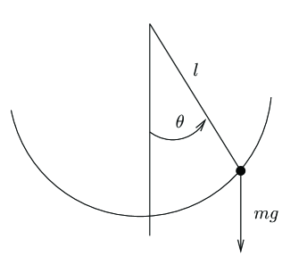
Figure 1: Pendulum.

$$ml\ddot{\theta}=-mg\sin\theta-kl\dot{\theta},$$

where $\theta$ denotes the angle subtended by the rod and the vertical axis through the pivot point, $l$ the length of the rod, $m$ the mass of the bob, $g$ the acceleration due to gravity, and $k$ the coefficient of friction. Let us take the state variables as $x_{1}=\theta$, and $x_{2}=\dot{\theta}$. Then the above equation is converted into a non-polynomial system

$$\left\{\begin{array}[]{l@{}l}\dot{x}_{1}=x_{2},\\ \dot{x}_{2}=-\frac{g}{l}\sin x_{1}-\frac{k}{m}x_{2}.\end{array}\right.$$

$\hfill\Box$

For the case of non-polynomial (control) systems, the problem of computing DOAs is still open, and only a few approaches have been proposed to deal with stability region analysis: in [3, 4, 5], the authors suggested a way to approximate non-polynomial vector fields by Taylor series expansion at the origin; in [23], an interval arithmetic approach for the estimation of the DOA was proposed; and recently, a method based on the theorem by Ehlich and Zeller was presented in [18, 17]. In this paper, we will apply polynomial approximation to transform a non-polynomial system into an uncertain polynomial system, whose set of trajectories contains that of the original non-polynomial system. Therefore, underestimate estimates of the DOA of the latter system yield those for the original non-polynomial system.

3 Polynomial Approximation

A key problem in estimating the DOA of a non-polynomial system is how to approximate the involved non-polynomial terms using polynomials, yielding an uncertain polynomial system with the equilibrium ${\mathbf{0}}$ being kept. This problem is further reduced to the following problem.

Problem 1

Let $\phi({\mathbf{x}}):\Psi\rightarrow{\mathbb{R}}$ be a non-polynomial function where $\Psi\subset{\mathbb{R}}^{n}$ is a bounded subset containing the origin ${\mathbf{0}}$. Given $d\in{\mathbb{Z}}_{\geq 0}$, we will find a polynomial $p({\mathbf{x}})$ with degree $d$ such that the error function $r_{d}({\mathbf{x}})=\phi({\mathbf{x}})-p({\mathbf{x}})$ satisfies $r_{d}({\mathbf{0}})=0$ and the value $\max_{{\mathbf{x}}\in\Psi}|r_{d}({\mathbf{x}})|$ is minimized.

The classic method of polynomial approximation is Taylor expansions. Suppose $\phi({\mathbf{x}})$ is a $d$ times continuously differentiable in $\Psi$. The Taylor expansion of $\phi({\mathbf{x}})$ at the origin ${\mathbf{0}}$ is

$$\phi({\mathbf{x}})=\underbrace{\sum_{|\alpha|\leq d-1}\frac{D^{\alpha}\phi({\mathbf{0}})}{\alpha!}{\mathbf{x}}^{\alpha}}_{p({\mathbf{x}})}+\underbrace{\sum_{|\beta|=d}\frac{D^{\beta}\phi(\xi)}{\beta!}{\mathbf{x}}^{\beta}}_{r_{d}({\mathbf{x}})}$$

for some $\xi\in(0,{\mathbf{x}})$. In the above expression, $p({\mathbf{x}})$ is an approximate polynomial of $\phi({\mathbf{x}})$ and the remainder term $r_{d}({\mathbf{x}})$ is the error function of this approximation. Clearly, if the size of the region $\Psi$ is small enough, the above Taylor expansion yields a tight bound of $r_{d}({\mathbf{x}})$ for all ${\mathbf{x}}\in\Psi$. However, when the size of $\Psi$ is large, the associated error bound may be too loose.

To obtain a tighter bound, we will apply multivariate polynomial interpolation ([9]) to compute an approximate polynomial $p({\mathbf{x}})$ of $\phi({\mathbf{x}})$ with a given degree $d$. Fix the graded lexicographic order in ${\mathbb{R}}[{\mathbf{x}}]$. For the function $\phi({\mathbf{x}})$, one may find the minimal monomial ${\mathbf{x}}^{\gamma}$ with $\gamma:=(\gamma_{1},\ldots,\gamma_{n})\in{{\mathbb{Z}}}_{\geq 0}^{n}$, such that $\lim_{{\mathbf{x}}\rightarrow{\mathbf{0}}}\frac{\phi({\mathbf{x}})-\phi({\mathbf{0}})}{{\mathbf{x}}^{\gamma}}\neq 0.$ Set $\psi({\mathbf{x}})=\frac{\phi({\mathbf{x}})-\phi({\mathbf{0}})}{{\mathbf{x}}^{\gamma}}.$ Let $d\in{\mathbb{Z}}_{\geq 0}$ be such that $d>|\gamma|:=\sum_{i=1}^{n}\gamma_{i}$. We construct a mesh $M$ on $\Psi$ with mesh spacing $s\in{\mathbb{R}}_{+}$ and mesh points set $\chi=\{{\mathbf{v}}_{1},{\mathbf{v}}_{2},\dots,{\mathbf{v}}_{k}\}$ where $k=\begin{pmatrix}n+d-|\gamma|\\ n\end{pmatrix}$. Like in [1], the meshes in our paper are either rectangular or simplicial. Then, we apply Lagrange interpolation to construct a polynomial $\tilde{p}({\mathbf{x}})$ as an approximation of $\psi({\mathbf{x}})$ through the interpolation points $\chi$, i.e., $\tilde{p}({\mathbf{v}}_{i})=\psi({\mathbf{v}}_{i}),\mbox{for }i=1,\dots,k.$ Next, we will compute a tight bound of the interpolation error function $\tilde{r}({\mathbf{x}}):=\psi({\mathbf{x}})-\tilde{p}({\mathbf{x}})$. Our idea is based on the following lemma.

Lemma 1

[26, Theorem 3] Let $K\subset{\mathbb{R}}^{n}$ be a convex polyhedron, and ${\mathbf{v}}_{1},{\mathbf{v}}_{2},\dots,{\mathbf{v}}_{k}$ and $s$ be the vertices and diameter of $K$ respectively. Suppose that $\varphi:K\rightarrow{\mathbb{R}}$ is a continuous and differential function on $K$, and $\lambda=\sup_{{\mathbf{x}}\in K}\|\bigtriangledown\varphi({\mathbf{x}})\|$. Then for all $a_{1},a_{2},\dots,a_{k}\in{\mathbb{R}}_{+}$ such that $a_{1}+a_{2}+\cdots+a_{k}=1$, we have

$$|\varphi({\mathbf{x}})-(a_{1}\varphi({\mathbf{v}}_{1})+a_{2}\varphi({\mathbf{v}}_{2})+\cdots+a_{k}\varphi({\mathbf{v}}_{k}))|\leq\frac{n}{n+1}\lambda s.$$

The following corollary gives an estimated bound of $\tilde{r}({\mathbf{x}})$ for ${\mathbf{x}}\in\Psi\cap M$.

Corollary 1

Let $s$ and $\chi:=\{{\mathbf{v}}_{1},{\mathbf{v}}_{2},\dots,{\mathbf{v}}_{k}\}$ be the mesh spacing and mesh points set of $M$, respectively. Suppose that $\tilde{p}({\mathbf{x}})$ is the interpolation polynomial of $\psi({\mathbf{x}})$ through $\chi$, and $\tilde{r}({\mathbf{x}})=\psi({\mathbf{x}})-\tilde{p}({\mathbf{x}})$ is the corresponding error function. Let $\lambda=\sup_{{\mathbf{x}}\in\Psi\cap M}\|\bigtriangledown\tilde{r}({\mathbf{x}})\|$. Then

$$|\tilde{r}({\mathbf{x}})|\leq\frac{n}{n+1}\lambda s\quad\mbox{ for all ${\mathbf{x}}\in M$}.$$

Proof.

Clearly, $\tilde{r}({\mathbf{x}})$ is a continuous and differential function on $M$, and

$$\tilde{r}({\mathbf{v}}_{1})=\tilde{r}({\mathbf{v}}_{2})=\cdots=\tilde{r}({\mathbf{v}}_{k})=0.$$

Thus, according to Lemma 1, for all $a_{1},a_{2},\dots,a_{v}\in{\mathbb{R}}_{+}$ such that $a_{1}+a_{2}+\cdots+a_{v}=1$,

$$\begin{split}|\tilde{r}({\mathbf{x}})-(a_{1}\tilde{r}({\mathbf{v}}_{1})+a_{2}\tilde{r}({\mathbf{v}}_{2})+\cdots+a_{k}\tilde{r}({\mathbf{v}}_{k}))|=|\tilde{r}({\mathbf{x}})|\leq\frac{n}{n+1}\lambda s.\end{split}$$

∎

Therefore, a non-polynomial function $\phi({\mathbf{x}})$ can be relaxed to an uncertain polynomial, as shown in the following theorem.

Theorem 1

For a non-polynomial function $\phi({\mathbf{x}})$ with ${\mathbf{x}}\in\Psi$, let ${\mathbf{x}}^{\gamma}$ with $\gamma\in{{\mathbb{Z}}}_{\geq 0}^{n}$ be the minimal monomial such that $\lim_{{\mathbf{x}}\rightarrow{\mathbf{0}}}\frac{\phi({\mathbf{x}})-\phi({\mathbf{0}})}{{\mathbf{x}}^{\gamma}}\neq 0$. Let $M$ be a mesh on $\Psi$ with mesh spacing $s\in{\mathbb{R}}_{+}$ and the mesh point set $\chi=\{{\mathbf{v}}_{1},{\mathbf{v}}_{2},\dots,{\mathbf{v}}_{k}\}$, in which $k=\begin{pmatrix}n+d-|\gamma|\\ n\end{pmatrix}$. Suppose that $\tilde{p}({\mathbf{x}})$ is the interpolation polynomial of $\psi({\mathbf{x}}):=\frac{\phi({\mathbf{x}})-\phi({\mathbf{0}})}{{\mathbf{x}}^{\gamma}}$ at $\chi$ with degree $\leq d-|\gamma|$, $\tilde{r}({\mathbf{x}})$ is the associated interpolation error function, and $\lambda=\sup_{{\mathbf{x}}\in\Psi\cap M}\|\bigtriangledown\tilde{r}({\mathbf{x}})\|$. Then for each ${\mathbf{x}}\in\Psi\cap M$ we have $\phi({\mathbf{x}})=p({\mathbf{x}})+r_{d}({\mathbf{x}}),$ where

$$p({\mathbf{x}})=\phi({\mathbf{0}})+\tilde{p}({\mathbf{x}})\,{\mathbf{x}}^{\gamma}\text{ and }r_{d}({\mathbf{x}})=u\,{\mathbf{x}}^{\gamma}\mbox{ with }|u|\leq\frac{n}{n+1}\lambda s.$$ (3)

Clearly, the bound of the error $r_{d}({\mathbf{x}})$ in (3) depends on the mesh spacing $s$, which can yield a tighter bound. Furthermore, the bound of $r_{d}({\mathbf{x}})$ in (3) will converge to zero if $d\rightarrow\infty$.

Example 2

Consider the function $\phi(x)=\cos x$ with $x\in\Psi=[-1.2,1.2]$. We want to compute a polynomial approximation for $\cos x$. Based on Theorem 1, we can obtain an uncertain polynomial with degree $6$, where

$$\left.\begin{array}[]{l@{}lr}&p(x)=1-0.5x^{2}+0.0416525x^{4}-0.00134386x^{6},&\\ &r_{6}(x)=ux^{2},\,\,-0.0000336\leq u\leq 0.0000336.&\Box\end{array}\right.$$

4 Computation of Domain of Attraction

In this section, we will consider an uncertain non-polynomial system of the form:

$$\dot{{\mathbf{x}}}={\mathbf{f}}({\mathbf{x}},\theta)\quad\mbox{ for all }\theta\in\Theta\subset{\mathbb{R}}^{t},$$ (4)

where $\theta$ denotes a vector of uncertainty. Assume that the equilibrium point of interest occurs at the origin ${\mathbf{0}}$, i.e, ${\mathbf{f}}({\mathbf{0}},\theta)={\mathbf{0}}$ for all $\theta\in\Theta$. Denote by $\phi(t;{\mathbf{x}}_{0},\theta)$ the solution of (4) for the initial value ${\mathbf{x}}(0)={\mathbf{x}}_{0}$ and the uncertainty $\theta$. The Domain of Attraction (DOA) of the system (4) is defined as

$$\{{\mathbf{x}}\in{\mathbb{R}}^{n}|\lim_{t\rightarrow\infty}\phi(t;{\mathbf{x}},\theta)={\mathbf{0}}\quad\mbox{for all }\theta\in\Theta\}.$$

Lemma 1 in [19] can be modified a bit to compute underestimates of the DOA for (4) through Lyapunov functions, as described in the following theorem.

Theorem 2

[22, Proposition 2.1] If there exists a continuously differentiable function $V:{\mathbb{R}}^{n}\rightarrow{\mathbb{R}}$ such that

$$\left\{\begin{array}[]{l@{}l}&\Omega_{V}:=\{{\mathbf{x}}\in{\mathbb{R}}^{n}:V({\mathbf{x}})\leq 1\}\text{ is bounded},\\ &V({{\mathbf{0}}})=0,\\ &V({\mathbf{x}})>0,\,\,\,\,\forall{\mathbf{x}}\in\Omega_{V}\backslash\{{\mathbf{0}}\},\\ &\dot{V}({\mathbf{x}})=\frac{\partial V}{\partial{\mathbf{x}}}\cdot{\mathbf{f}}({\mathbf{x}},\theta)<0,\,\,\,\,\forall{\mathbf{x}}\in\Omega_{V}\backslash\{{\mathbf{0}}\},\,\forall\theta\in\Theta\end{array}\right.$$

then $\Omega_{V}$ is an invariant subset of the DOA.

When the equilibrium ${\mathbf{0}}$ is asymptotically stable, the set $\Omega_{c}$ is clearly an underestimate of the DOA since every trajectory starting in $\Omega_{c}$ remains in $\Omega_{c}$ and approaches ${\mathbf{0}}$ as $t\rightarrow\infty$. And, if the equilibrium ${\mathbf{0}}$ is globally asymptotically stable then the DOA will be the whole space ${\mathbb{R}}^{n}$.

To enlarge the estimate $\Omega_{V}$ given in Theorem 2, [19] defined a variable sized region

$$P_{\beta}=\{{\mathbf{x}}\in{\mathbb{R}}^{n}:g({\mathbf{x}})\leq\beta\}$$

with $g({\mathbf{x}})$ a fixed and positive definite polynomial in ${\mathbb{R}}[{\mathbf{x}}]$, for instance, $g({\mathbf{x}})=\sum_{i=1}^{n}x_{i}^{2}$, and maximize $\beta$ subject to the constraint $P_{\beta}\subseteq\Omega_{V}$ and the constraints in Theorem 2. Thus, the problem of computing $\Omega_{V}$ can be transformed into the following problem:

$$\left.\begin{array}[]{l@{}l}&\displaystyle\max\beta\\ &\text{s.t.}\,\,\,\Omega_{V}\text{ is bounded},\\ &\quad\,\,\,V({\mathbf{0}})=0,\\ &\quad\,\,\,V({\mathbf{x}})>0,\,\,\,\,\forall{\mathbf{x}}\in\Omega_{V}\backslash\{{\mathbf{0}}\},\\ &\quad\,\,\,\dot{V}({\mathbf{x}})=\frac{\partial V}{\partial{\mathbf{x}}}\cdot{\mathbf{f}}({\mathbf{x}},\theta)<0,\,\,\,\,\forall{\mathbf{x}}\in\Omega_{V}\backslash\{{\mathbf{0}}\},\,\forall\theta\in\Theta\\ &\quad\,\,\,g({\mathbf{x}})\leq\beta\models V({\mathbf{x}})\leq 1.\end{array}\right\}$$ (11)

Suppose that the non-polynomial system (4) has the following form

$$\dot{x}_{i}=f_{i}({\mathbf{x}},\theta)=f_{i0}({\mathbf{x}},\theta)+\sum_{j=1}^{k}f_{ij}({\mathbf{x}},\theta)\phi_{ij}({\mathbf{x}}),\quad i=1,\dots,n,$$ (12)

where $f_{ij}:{\mathbb{R}}^{n}\times{\mathbb{R}}^{t}\rightarrow{\mathbb{R}}$ are polynomials in ${\mathbf{x}}$ for $j=0,\dots,k$, and $\phi_{ij}:{\mathbb{R}}^{n}\rightarrow{\mathbb{R}}$ are non-polynomial functions for $j=1,\dots,k$. Using the polynomial approximation technique in Section 3, we can replace each non-polynomial term $\phi_{ij}({\mathbf{x}})$ by an uncertain polynomial $p_{ij}({\mathbf{x}})+u_{ij}{\mathbf{x}}^{\gamma_{ij}}$ with the bound $|u_{ij}|\leq b_{ij}$. This gives rise to the following uncertain polynomial system:

$$\dot{x}_{i}=\hat{f}_{i}({\mathbf{x}},\theta)=f_{i0}({\mathbf{x}},\theta)+\sum_{j=1}^{k}f_{ij}({\mathbf{x}},\theta)(p_{ij}({\mathbf{x}})+u_{ij}{\mathbf{x}}^{\gamma_{ij}})$$ (13)

where $|u_{ij}|\leq b_{ij}$ for $i=1,\dots,n$. It is not hard to prove that the set of all trajectories of the system (12) is a subset of that of the system (13), and, consequently, the DOA of (13) is actually a subset of that of the system (12). Furthermore, the tighter the bound $b_{ij}$ is, the closer the DOA of (13) is to the DOA of the original system.

Next, we consider how to find an optimal estimate of the DOA for the uncertain system (12) through computing the $\Omega_{V}$ in (11). Remark that the constraint $\dot{V}({\mathbf{x}})=\frac{\partial V}{\partial{\mathbf{x}}}\cdot{\mathbf{f}}({\mathbf{x}},\theta)<0$ in (12) may involve non-polynomial terms due to the existence of $\phi_{ij}({\mathbf{x}})$’s. In this situation, replacing the above constraint by $\dot{V}({\mathbf{x}})=\frac{\partial V}{\partial{\mathbf{x}}}\cdot\hat{\mathbf{f}}({\mathbf{x}},\theta)<0$, the problem (11) can be relaxed as follow.

Theorem 3

Let $\hat{\mathbf{f}}({\mathbf{x}},\theta)=(\hat{f}_{1}({\mathbf{x}},\theta),\dots,\hat{f}_{n}({\mathbf{x}},\theta))^{T}$ with $\hat{f}_{i}({\mathbf{x}},\theta)$ given in (13). If $\widetilde{V}({\mathbf{x}})$ is a solution of the following polynomial optimization

$$\left.\begin{array}[]{l@{}l}&\displaystyle\max_{V,\beta}\ \beta\\ &\text{s.t.}\,V({\mathbf{0}})=0,\\ &\quad V({\mathbf{x}})>0\quad\forall{\mathbf{x}}\in\Omega_{V}\backslash\{{\mathbf{0}}\},\\ &\,\,\,\frac{\partial V}{\partial{\mathbf{x}}}\cdot\hat{{\mathbf{f}}}({\mathbf{x}},\theta)<0\,\forall{\mathbf{x}}\in\Omega_{V}\backslash\{{\mathbf{0}}\},\forall\theta\in\Theta,\forall u_{ij}\in\{\pm b_{ij}\},\\ &\quad g({\mathbf{x}})\leq\beta\models V({\mathbf{x}})\leq 1,\end{array}\right\}$$ (19)

then $\Omega_{\widetilde{V}}:=\{{\mathbf{x}}\in{\mathbb{R}}^{n}:\widetilde{V}({\mathbf{x}})\leq 1\}$ is an invariant subset of the DOA for (13), and therefore an invariant subset of DOA for (12).

Proof.

By construction of $\hat{f}_{i}({\mathbf{x}},\theta)$’s, we have

$$\small\begin{split}\forall{\mathbf{x}}\in\Omega_{V}\backslash\{{\mathbf{0}}\},\forall\theta\in\Theta,\,\,\exists\tilde{u}_{ij}\in[-b_{ij},b_{ij}]:\dot{V}({\mathbf{x}})=\frac{\partial{V}}{\partial{\mathbf{x}}}\cdot\hat{{\mathbf{f}}}({\mathbf{x}},\theta).\end{split}$$

Clearly, if the constraints in (19) are fulfilled, the conditions in (11) also hold. Therefore, $\Omega_{\widetilde{V}}$ is certainly a subset of $\Omega_{V}$ in (11). ∎

Assume that $\Theta$ is a semialgebraic set. For simplicity, we suppose $\Theta=\{\theta\in\Theta:\psi(\theta)\geq 0\}.$ By rewriting the third, fourth and fifth constraints into equivalent empty set conditions, the condition (19) is transformed as

$$\left\{\begin{array}[]{l@{}l}&V({\mathbf{0}})=0,\\ &\{{\mathbf{x}}\in{\mathbb{R}}^{n}:V({\mathbf{x}})\leq 1,{\mathbf{x}}\neq{\mathbf{0}},V({\mathbf{x}})\leq 0\}=\emptyset,\\ &\{{\mathbf{x}}\in{\mathbb{R}}^{n}:V({\mathbf{x}})\leq 1,{\mathbf{x}}\neq{\mathbf{0}},\psi(\theta)\geq 0,\frac{\partial V}{\partial{\mathbf{x}}}\cdot\hat{{\mathbf{f}}}({\mathbf{x}})\geq 0\}=\emptyset,\forall u_{ij}\in\{\pm b_{ij}\},\\ &\{{\mathbf{x}}\in{\mathbb{R}}^{n}:g({\mathbf{x}})\leq\beta,V({\mathbf{x}})\geq 1,V({\mathbf{x}})\neq 1\}=\emptyset.\end{array}\right.$$ (24)

As stated in [19], Stengle’s Positivstellensatz [2] be applied directly to solve (24). However, from the computational point of view, it is more efficient to replace all the inequations in (24) by inequalities of the form $f\geq 0$ or $f\leq 0$. This can be done by introducing constants $\delta\in{\mathbb{R}}_{+}$ and polynomials of the form [19] $l({\mathbf{x}})=\Sigma_{i=1}^{n}\epsilon_{i}x_{i}^{m},$ where $\epsilon_{i}\in{\mathbb{R}}_{+}$ and $m$ is assumed to be even. For example, by using $\delta_{1}$ and $l_{1}({\mathbf{x}})$, the second condition in (24) can be relaxed as

$$\{{\mathbf{x}}\in{\mathbb{R}}^{n}:V({\mathbf{x}})-1\leq 0,V({\mathbf{x}})-l_{1}({\mathbf{x}})+\delta_{1}\leq 0\}=\emptyset.$$

Therefore, the problem (24) can be transformed into the following feasibility problem:

$$\left.\begin{array}[]{l@{}l}&\displaystyle\max_{V,\beta}\ \beta\\ &\text{s.t.}\,V({\mathbf{0}})=0,\\ &\,\,\,\{{\mathbf{x}}\in{\mathbb{R}}^{n}:V({\mathbf{x}})-1\leq 0,V({\mathbf{x}})-l_{1}({\mathbf{x}})+\delta_{1}\leq 0\}=\emptyset,\\ &\,\,\,\{{\mathbf{x}}\in{\mathbb{R}}^{n}:V({\mathbf{x}})-1\leq 0,-\frac{\partial V}{\partial{\mathbf{x}}}\cdot\hat{{\mathbf{f}}}({\mathbf{x}},\theta)-l_{2}({\mathbf{x}})+\delta_{2}\leq 0,\psi(\theta)\geq 0\}=\emptyset,\,\,\forall u_{ij}\in\{\pm b_{ij}\}\\ &\,\,\,\{{\mathbf{x}}\in{\mathbb{R}}^{n}:g({\mathbf{x}})-\beta\leq 0,V({\mathbf{x}})-1-\delta_{3}\geq 0\}=\emptyset.\end{array}\right\}$$

Suppose that $\Sigma[{\mathbf{x}}]$ is the set of sum of squares (SOS) polynomials in ${\mathbb{R}}[{\mathbf{x}}]$. Since the constraints in the above problem involve no equations and inequations, only a special case of Stengle’s Positivstellensatz is needed, as shown in the following corollary.

Corollary 2

Let $F=\{f_{i}\}_{i=1,\dots,r}$ be a set of polynomials in ${\mathbb{R}}[{\mathbf{x}}]$. The semi-algebraic set

$$\{{\mathbf{x}}\in{\mathbb{R}}^{n}:f_{i}({\mathbf{x}})\geq 0,i=1,\dots,r\}$$

is empty if and only if there exist polynomials $s_{0},s_{1},\dots,s_{l}\in\Sigma[{\mathbf{x}}]$ such that

$$s_{0}+\sum_{j=1}^{l}s_{j}b_{j}=0$$

where $b_{j}\in\left\{f_{1}^{t_{1}}\cdots f_{r}^{t_{r}}:t_{i}\in{\mathbb{Z}}_{\geq 0}\right\}$.

Applying Corollary 2, and removing all the crossing products of the involved inequalities, we obtain the following relaxed problem:

$$\left.\begin{array}[]{l@{}l}&\displaystyle\max_{V,\beta}\ \beta\\ &\text{s.t.}\,V({\mathbf{0}})=0,\\ &\quad\sigma_{0}({\mathbf{x}})+\sigma_{1}({\mathbf{x}})(1-V({\mathbf{x}}))+\sigma_{2}({\mathbf{x}})(-V({\mathbf{x}})+l_{1}({\mathbf{x}})-\delta_{1})=0,\\ &\quad\lambda_{0}({\mathbf{x}})+\lambda_{1}({\mathbf{x}})(1-V({\mathbf{x}}))+\lambda_{2}({\mathbf{x}})(\frac{\partial V}{\partial{\mathbf{x}}}\cdot\hat{{\mathbf{f}},\theta}({\mathbf{x}})+l_{2}({\mathbf{x}})-\delta_{2})=0,\\ &\quad\rho_{0}({\mathbf{x}})+\rho_{1}({\mathbf{x}})(\beta-g({\mathbf{x}}))+\rho_{2}({\mathbf{x}})(V({\mathbf{x}})-1-\delta_{3})=0,\end{array}\right\}$$ (31)

with $\sigma_{\iota}({\mathbf{x}}),\lambda_{\iota}({\mathbf{x}}),\rho_{\iota}({\mathbf{x}})\in\Sigma[{\mathbf{x}}],\iota=0,\dots,2$ and for any $u_{ij}\in\{\pm b_{ij}\}$.

Suppose that the Lyapunov function $V({\mathbf{x}})$ to be computed is a polynomial of degree $d$ and has the form $V({\mathbf{x}})=\sum_{\alpha}c_{\alpha}{\mathbf{x}}^{\alpha}$ where $c_{\alpha}\in{\mathbb{R}}$, ${\mathbf{x}}^{\alpha}=x_{1}^{\alpha_{1}}\cdots x_{n}^{\alpha_{n}}$ and $\alpha=(\alpha_{1},\ldots,\alpha_{n})\in{{\mathbb{Z}}}_{\geq 0}^{n}$ with $\sum_{i=1}^{n}\alpha_{i}\leq d$. The decision variables of the problem (31) are $\beta$ and the coefficients of all the unknown polynomials occurred in (31), such as $V({\mathbf{x}}),\sigma_{\iota}({\mathbf{x}}),$ $\lambda_{\iota}({\mathbf{x}})$ and $\rho_{\iota}({\mathbf{x}})$. Clearly, some nonlinear terms which are products of the undetermined coefficients will occur in (31), which yields a non-convex bilinear matrix inequalities (BMI) problem. To solve BMI problems, either a Matlab package PENBMI solver [13], which combines the (exterior) penalty and (interior) barrier method with the augmented Lagrangian method, can be applied directly, or an iterative method can be applied by fixing $\beta$ and the polynomials alternatively, which leads to a sequential convex LMI problem. The reader can refer to [25] for more details.

Remark that, the above proposed method is also applicable to computing the largest possible estimate of the DOA for a non-polynomial system (1) at ${\mathbf{0}}$ through a fixed Lyapunov function $V({\mathbf{x}})$. Let $\Omega_{c}:=\{{\mathbf{x}}\in{\mathbb{R}}^{n}:V({\mathbf{x}})\leq c\}.$ We will compute

$$\Omega_{c^{*}}=\{{\mathbf{x}}\in{\mathbb{R}}^{n}:V({\mathbf{x}})\leq c^{*}\},$$

where $c^{*}=\sup\{c\in{\mathbb{R}}:\dot{V}({\mathbf{x}})<0,\,\,\forall{\mathbf{x}}\in\Omega_{c}\setminus\{{\mathbf{0}}\}\}.$ Due to the existence of non-polynomial terms, $c^{*}$ cannot be computed explicitly. Instead, we will compute the lower and upper bounds of $c^{*}$ as follows. Replacing the involved non-polynomial $\phi_{ij}$ by uncertain polynomials, computing the lower bound $c_{d}$ of $c^{*}$ can be relaxed as the following problem:

$$\left.\begin{array}[]{l@{}l}&\displaystyle c_{d}=\max_{c,{\mathbf{x}}}\,\,c\\ &\quad\text{s.t.}\,\,\frac{\partial V}{\partial{\mathbf{x}}}\cdot\hat{{\mathbf{f}}}({\mathbf{x}})<0,\,\,\forall{\mathbf{x}}\in\Omega_{c}\backslash\{{\mathbf{0}}\},\,\,\forall u_{ij}\in\{\pm b_{ij}\},\end{array}\right.$$ (34)

where $d$ is the degree of the interpolation polynomials. Clearly, $c_{d}$ will converge to $c^{*}$ when $d$ tends to $\infty$. Next, we will search for a tight upper bound $\upsilon_{d}$ of $c^{*}$. To achieve this, let us look for $\upsilon_{d}$ such that, for each $u_{ij}\in\{\pm b_{ij}\}$, the constant semi-algebraic system

$$V({\mathbf{x}})-\upsilon_{d}\leq 0\wedge{\mathbf{x}}\neq{\mathbf{0}}\wedge\frac{\partial V}{\partial{\mathbf{x}}}\cdot\hat{{\mathbf{f}}}({\mathbf{x}})\geq 0$$ (35)

has real solutions, which implies that $\Omega_{\upsilon_{d}}$ is not an estimate of the DOA. Based on bisection, $\upsilon_{d}$ can be computed by Maple packages RegularChains, DISCOVERER [24] and RAGLib [14].

5 Experiments

Let us present some examples of DOA analysis of non-polynomial systems.

Example 3

[4, Example 1] Consider a non-polynomial system

$$\left\{\begin{array}[]{l@{}l}\dot{x}_{1}=-x_{1}+x_{2}+0.5(e^{x_{1}}-1),\\ \dot{x}_{2}=-x_{1}-x_{2}+x_{1}x_{2}+x_{1}\cos x_{1}.\end{array}\right.$$

To estimate the DOA of this system, we need to approximate the occurred non-polynomial terms $e^{x_{1}}$ and $\cos x_{1}$ by uncertain polynomials. Based on the technique in Section 3, we obtain

$$\left\{\begin{array}[]{l@{}l}&e^{x_{1}}=1+(1.0000004+u_{1})x_{1}+\cdots+0.0014482244x_{1}^{6},\\ &\cos x_{1}=1-(0.5+u_{2})x_{1}^{2}+0.041669352x_{1}^{4}-0.0013878601x_{1}^{6},\\ &-0.6\leq x_{1}\leq 0.6,\\ &-3\times 10^{-6}\leq u_{1}\leq 3\times 10^{-6},\\ &-1.2\times 10^{-6}\leq u_{2}\leq 1.2\times 10^{-6},\end{array}\right.$$

and the associated uncertain polynomial system.

We first consider a fixed Lyapunov function $V(x_{1},x_{2})=x_{1}^{2}+x_{2}^{2}$. For the given degree $6$ of interpolation polynomials, after solving the corresponding SOS programming (34), we obtain the lower bound $c_{6}=0.321064$ of $c^{*}$, which is an improvement over the results in [4] with the lower bound 0.3210. Furthermore, by solving the problem (35) we obtain a tight upper bound $\upsilon_{6}=0.3216$ of $c^{*}$.

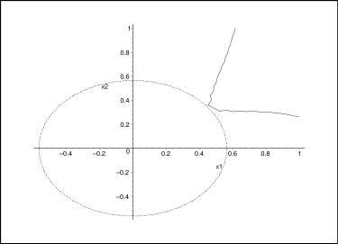
(a) boundaries of $\Omega_{c_{6}}$ with $c_{6}=0.321064$ and $\dot{V}=0$

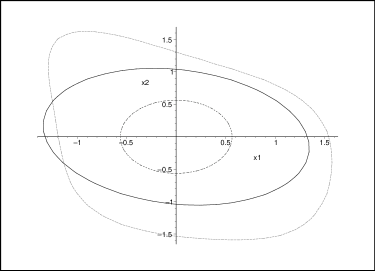
(b) boundaries of the estimates for $\deg{V=2}$ and $\deg{V=4}$

Figure 2: Results of Example 4.

Next, we estimate the DOA with variable Lyapunov functions. Suppose $g(x_{1},x_{2})=x_{1}^{2}+x_{2}^{2}$. For $\deg V=2$, solving the SOS programming (31) with BMI constraints yields

$$\begin{split}&{V}(x_{1},x_{2})=0.56678683x_{1}^{2}+0.23598133x_{1}x_{2}+0.92086339x_{2}^{2},\\ &{\beta}=1.0453916,\end{split}$$

which is an improvement over the result from [4] where ${\beta}=1.0404$. Similarly, for $\deg V=4$ solving the SOS programming (31) with BMI constraints yields ${\beta}=1.4001306$ and

$${V}(x_{1},x_{2})=0.068693712x_{1}^{2}+\cdots+0.27723966x_{1}^{4}+0.2167918x_{2}^{4},$$

which is an improvement over the result from [4] where ${\beta}=1.2769$. Therefore, $\Omega_{V}$ is an estimate of the DOA of the given system. Figure 2 shows the results obtained with Lyapunov functions of degrees 2 and 4. $\hfill\Box$

Example 4

[4, Example 2]Consider a non-polynomial system

$$\left\{\begin{array}[]{l@{}l}\dot{x}_{1}=x_{2},\\ \dot{x}_{2}=-0.2x_{2}+0.81\sin x_{1}\cos x_{1}-\sin x_{1}.\end{array}\right.$$

Using the technique in Section 3, we obtain the approximations of the non-polynomial terms $\sin x_{1}$ and $\cos x_{1}$ as follows

$$\left\{\begin{array}[]{l@{}l}&\sin 2x_{1}=(2+u_{1})x_{1}-1.3333091x_{1}^{3}+0.26625372x_{1}^{5}-0.023889715x_{1}^{7},\\ &\sin x_{1}=(1+u_{2})x_{1}-0.16666643x_{1}^{3}+0.008331760x_{1}^{5}-0.00019471928x_{1}^{7},\\ &-0.84\leq x_{1}\leq 0.84,\\ &-5.4\cdot 10^{-5}\leq u_{1}\leq 5.4\cdot 10^{-5},\\ &-1\cdot 10^{-7}\leq u_{2}\leq 1\cdot 10^{-7},\end{array}\right.$$

and the associated uncertain polynomial system.

We first fix the Lyapunov function $V(x_{1},x_{2})=x_{1}^{2}+x_{1}x_{2}+4x_{2}^{2}$. Let the degree of interpolation polynomials be 7. Solving the corresponding SOS programming (34), we obtain the results for the lower bound $c_{7}=0.69922$ of $c^{*}$, which is an improvement over the result from [4] where the lower bound was 0.6990. Furthermore, by solving the problem (35) we obtain a tighter upper bound $\upsilon_{7}=0.6998$ of $c^{*}$.

We then estimate the DOA with variable Lyapunov functions. Suppose $g(x_{1},x_{2})=x_{1}^{2}+x_{2}^{2}$. When $\deg V=2$, by solving the SOS programming (31) with BMI constraints, we obtain

$$\begin{split}&{V}(x_{1},x_{2})=1.01636667x_{1}^{2}+0.84993333x_{1}x_{2}+3.40233333x_{2}^{2},\\ &{\beta}=0.287706,\end{split}$$

which is an improvement over the result from [4] where ${\beta}=0.2809$. Similarly, when $\deg V=4$, by solving the SOS programming (31) with BMI constraints, we obtain ${\beta}=1.92156$ and

$${V}(x_{1},x_{2})=0.053849691x_{1}^{2}+\cdots+0.11144243x_{1}^{4}+0.058855229x_{2}^{4},$$

which is an improvement over the result from [4] where ${\beta}=1.1236$. Therefore, $\Omega_{\widetilde{V}}$ is an estimate of the DOA of the given system. Figure 3 shows the results obtained with Lyapunov functions of degrees 2 and 4.

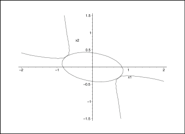
(a) boundaries of $\Omega_{c_{7}}$ with $c_{7}=0.69922$ and $\dot{V}=0$

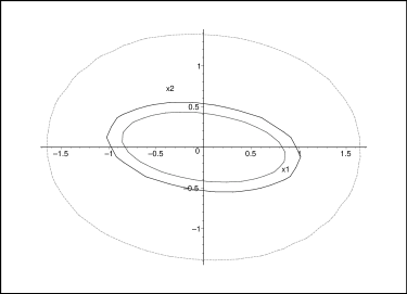
(b) boundaries of the estimates for $\deg{V=2}$ and $\deg{V=4}$

Figure 3: Results of Example 5.

$\hfill\Box$

Example 5

[12, Example 2.2] Consider an uncertain non-polynomial system

$$\left\{\begin{array}[]{l@{}l}\dot{x}_{1}=x_{2},\\ \dot{x}_{2}=-\theta x_{2}-10\sin x_{1},\end{array}\right.$$

for $0.2\leq\theta\leq 1$. Based on the technique in Section 3, we obtain an approximation of the non-polynomial term $\sin x_{1}$ as follows

$$\left\{\begin{array}[]{l@{}l}&\sin x_{1}=(1+u_{1})x_{1}-0.1666426901x_{1}^{3}+0.008282118073x_{1}^{5}-0.0001751721223x_{1}^{7},\\ &-2.4\leq x_{1}\leq 2.4,\\ &-4.365606\times 10^{-4}\leq u_{1}\leq 4.365606\times 10^{-4},\end{array}\right.$$

and the associated uncertain polynomial system.

Suppose $g(x_{1},x_{2})=x_{1}^{2}+x_{2}^{2}$. For $\deg V=4$, solving the SOS programming (31) with BMI constraints yields ${\beta}=0.66552836$ and

$${V}(x_{1},x_{2})=1.1629845x_{1}^{2}+\cdots+0.51014802x_{1}^{4}+0.010528x_{2}^{4}.$$

Then $\Omega_{{V}}$ is an estimate of the DOA of the given system. $\hfill\Box$

6 Conclusion

In this paper, we present a method on stability region analysis of non-polynomial systems via Lyapunov functions. A polynomial approximation technique, based on multivariate polynomial interpolation and error analysis, is applied to compute an uncertain polynomial system, whose set of trajectories contains that of the original non-polynomial system. To estimate DOA of the uncertain polynomial system, we apply Positivstellensatz to transform polynomial optimization problem into the corresponding (bilinear) sum of squares programming, which can be solved using the PENBMI solver or iterative method. Experiments on the benchmark non-polynomial systems show that our approach provides better estimates.

References

- [1] Asarin, E., Dang, T., and Girard, A. Reachability analysis of nonlinear systems using conservative approximation. In Proceedings of the 6th International Conference on Hybrid Systems: Computation and Control (2003), Springer-Verlag, pp. 20–35.
- [2] Bochnak, J., Coste, M., and Roy, M. Real Algebraic Geometry. Springer Verlag, 1998.
- [3] Chesi, G. Domain of attraction: estimates for non-polynomial systems via LMIs. In Proc. 16th IFAC World Congress on Automatic Control (2005).
- [4] Chesi, G. Estimating the domain of attraction for non-polynomial systems via LMI optimizations. Automatica 45, 6 (2009), 1536–1541.
- [5] Chesi, G. Domain of Attraction: Analysis and Control via SOS Programming. Springer, 2011.
- [6] Chesi, G., Garulli, A., Tesi, A., and Vicino, A. LMI-based computation of optimal quadratic Lyapunov functions for odd polynomial systems. International Journal of Robust and Nonlinear Control 15, 1 (2005), 35–49.
- [7] Chiang, H., and Thorp, J. Stability regions of nonlinear dynamical systems: A constructive methodology. IEEE Transaction on Automatic Control 34, 12 (1989), 1229–1241.
- [8] Cruck, E., Moitie, R., and Seube, N. Estimation of basins of attraction for uncertain systems with affine and Lipschitz dynamics. Dynamics and Control 11, 3 (2001), 211–227.
- [9] Gasca, M., and Sauer, T. On the history of multivariate polynomial interpolation. Journal of Computational and Applied Mathematics 122, 1 (2000), 23–35.
- [10] Hachicho, O., and Tibken, B. Estimating domains of attraction of a class of nonlinear dynamical systems with LMI methods based on the theory of moments. In Proceedings of the 41st IEEE Conference on Decision and Control (2002), vol. 3, IEEE, pp. 3150–3155.
- [11] Jarvis-Wloszek, Z. Lyapunov Based Analysis and Controller Synthesis for Polynomial Systems Using Sum-Of-Squares Optimization. PhD thesis, University of California, 2003.
- [12] Khalil, H. Nonlinear Systems, Third ed. New Jewsey, Prentice hall, 2002.
- [13] Kočvara, M., and Stingl, M. PENBMI User’s Guide (Version 2.0). Available at http://www.penopt.com, 2005.
- [14] Mohab, S. E. D. Raglib (Real Algebraic Library Maple package). Available at http://www-calfor.lip6.fr/~safey/RAGLib, 2003.
- [15] Prajna, S., Parrilo, P., and Rantzer, A. Nonlinear control synthesis by convex optimization. IEEE Transactions on Automatic Control 49, 2 (2004), 310–314.
- [16] Prakash, S., Vanualailai, J., and Soma, T. Obtaining approximate region of asymptotic stability by computer algebra: A case study. The South Pacific Journal of Natural and Applied Sciences 20, 1 (2002), 56–61.
- [17] Saleme, A., and Tibken, B. A new method to estimate a guaranteed subset of the domain of attraction for non-polynomial systems. In American Control Conference (2012), IEEE, pp. 2577–2582.
- [18] Saleme, A., Tibken, B., Warthenpfuhl, S., and Selbach, C. Estimation of the domain of attraction for non-polynomial systems: A novel method. In Proceedings of the 18th IFAC World Congress, Milano, Italy (2011), pp. 10976–10981.
- [19] Tan, W., and Packard, A. Stability region analysis using sum of squares programming. In American Control Conference (2006), IEEE, pp. 2297–2302.
- [20] Tibken, B. Estimation of the domain of attraction for polynomial systems via LMIs. In Proceedings of the 39th IEEE Conference on Decision and Control (2000), vol. 4, IEEE, pp. 3860–3864.
- [21] Tibken, B., and Dilaver, K. Computation of subsets of the domain of attraction for polynomial systems. In Proceedings of the 41st IEEE Conference on Decision and Control (2002), vol. 3, IEEE, pp. 2651–2656.
- [22] Topcu, U., Packard, A. K., Seiler, P., and Balas, G. J. Robust region-of-attraction estimation. IEEE Transactions on Automatic Control 55, 1 (2010), 137–142.
- [23] Warthenpfuhl, S., Tibken, B., and Mayer, S. An interval arithmetic approach for the estimation of the domain of attraction. In IEEE International Symposium on Computer-Aided Control System Design (2010), IEEE, pp. 1999–2004.
- [24] Xia, B. DISCOVERER: A tool for solving semi-algebraic systems. ACM Commun. Compute. Algebra 41, 3 (2007), 102–103.
- [25] Yang, Z., Wu, M., and Lin, W. Exact verification of hybrid systems based on bilinear SOS representation. Submitted, 19 pages, 2012.
- [26] Zeng, Z., and Zhang, J. A mechanical proof to a geometric inequality of Zirakzadeh through rectangular partition of polyhedra (in Chinese). Journal of Systems Science and Mathematical Sciences 30, 11 (2010), 1430–1458.