Higgs diphoton rate and mass enhancement with vector-like leptons and the scale of supersymmetry

Abstract

Analysis of contributions from vector-like leptonic supermultiplets to the Higgs diphoton decay rate and to the Higgs boson mass is given. Corrections arising from the exchange of the new leptons and their super-partners, as well as their mirrors are computed analytically and numerically. We also study the correlation between the enhanced Higgs diphoton rate and the Higgs mass corrections. Specifically, we find two branches in the numerical analysis: on the lower branch the diphoton rate enhancement is flat while on the upper branch it has a strong correlation with the Higgs mass enhancement. It is seen that a factor of 1.4-1.8 enhancement of the Higgs diphoton rate on the upper branch can be achieved, and a 4-10 GeV positive correction to the Higgs mass can also be obtained simultaneously. The effect of this extra contribution to the Higgs mass is to release the constraint on weak scale supersymmetry, allowing its scale to be lower than in the theory without extra contributions. The vector-like supermultiplets also have collider implications which could be testable at the LHC and at the ILC.

^a Department of Physics and Institute for Advanced Study,

The Hong Kong University of Science and Technology, Hong Kong

^b Department of Physics, Northeastern University, Boston, MA 02115, USA

1 Introduction

Recently the ATLAS and the CMS Collaborations using the combined 7 TeV and 8 TeV data found a signal for a boson with the ATLAS finding a signal at $126.0\pm 0.4({\rm stat})\pm 0.4({\rm sys})~{}{\rm GeV}$ at the $5.0\sigma$ level [1] and the CMS finding a signal at $125.3\pm 0.4({\rm stat})\pm 0.5({\rm sys})~{}{\rm GeV}$ at the $5.0\sigma$ level [2]. While the properties of this boson still need to be fully established there is the general belief that it is indeed the long sought after Higgs boson [3, 4, 5] of the electroweak theory [6, 7]. In the analysis below we will assume that the observed boson is indeed the Higgs particle that is remnant of the electroweak symmetry breaking. It is pertinent to observe that the results of the ATLAS and CMS Collaborations are remarkably consistent with the predictions of supergravity grand unified models [8, 9, 10, 11] with radiative electroweak symmetry breaking (for a review see [12]) which predict the Higgs boson mass to lie below around $130$ GeV [13, 14, 15, 16, 17] (For a recent review of Higgs and supersymmetry see [18]). However, the fact that the Higgs mass lies close to the upper limit of the prediction of the supergravity unification within the Minimal Supersymmetric Standard Model (MSSM) indicates that the loop correction to the Higgs boson mass is rather large which in turn implies that the existence of a high scale of supersymmetry, specifically a high scale for the squarks. However, corrections on the order of a few GeVs from a source external to MSSM can significantly lower the scale of supersymmetry. Here we investigate this possibility by considering an extension of MSSM with vector-like leptonic supermultiplets. The assumption of additional vector-like leptonic supermultiplets will not alter the Higgs production cross section and is not strongly constrained by the electroweak data.

Aside from the relative heaviness of the Higgs boson is the issue of any possible deviations of the Higgs boson couplings from the ones predicted in the Standard Model. If a significant deviation from the Standard Model prediction is seen, it would indicate the existence of new physics. However, it would take a considerable amount of luminosity, i.e., as much as 3000 fb^-1 at LHC14 to achieve an accuracy of 10-20% [19] in the determination of the Higgs couplings with fermions and with dibosons. An exception to the above is the diphoton channel for which the background is remarkably small and it was the discovery channel for the Higgs boson. Here the current data gives some hint of a possible deviation from the Standard Model prediction. The ATLAS and the CMS Collaborations give [2, 1]:

$$R_{\gamma\gamma}\equiv\frac{\sigma(pp\to h)_{\rm obs}}{\sigma(pp\to h)_{\rm SM}}\cdot\frac{\Gamma(h\to\gamma\gamma)_{\rm obs}}{\Gamma(h\to\gamma\gamma)_{\rm SM}}=1.8\pm 0.5~{}({\rm ATLAS}),~{}1.6\pm 0.4~{}({\rm CMS}),$$ (1)

where

$$\frac{\sigma(pp\to h)_{\rm obs}}{\sigma(pp\to h)_{\rm SM}}=1.4\pm 0.3{\rm~{}(ATLAS)},~{}0.87\pm 0.23{\rm~{}(CMS)}.$$ (2)

In the Standard Model the largest contribution to the $h\to\gamma\gamma$ mode arises from the $W^{+}W^{-}$ in the loop and this contribution is partially cancelled by the contribution arising from the top quark in the loop. If this observed enhancement is not due to QCD uncertainties [20], one needs new contributions beyond the standard model to increase the diphoton rate. There are many works which have investigated this possibility, and an enhancement of the diphoton rate can be achieved in many ways: from light staus with large mixing [21, 22, 23, 24], from extra vector-like leptons [25, 26, 27, 28, 29, 30, 31] and through other mechanisms [32, 33, 34, 35, 36, 37, 38, 39, 40, 41, 42, 43, 44, 45, 46, 47]. Additional papers where vector-like fermions have been discussed are [48, 49, 50, 51, 52]. Most of these works are within non-supersymmetric framework. However, with 125 GeV Higgs mass, vacuum stability is a serious problem in most models. Thus, for example, in the Standard Model vacuum stability up to the Planck scale may not be achievable since analysis using next-to-next-leading order correction require that $m_{h}>129.4$ GeV for the vacuum to be absolutely stable up to the Planck scale [53] (see, however, [54, 55]). For this reason we consider supersymmetric models which are less problematic with regard to vacuum stability (see e.g., [28, 56, 57, 58]). Additionally, the supersymmetric theories also avoid the well-known fine-tuning problems of non-supersymmetric theories. An analysis to determine whether a significant diphoton enhancement can be achieved in MSSM was carried out in [59, 60].

In this work, we consider effects from additional vector-like leptonic multiplets in loops both to the Higgs diphoton rate and to the Higgs mass in a supersymmetric framework. Vector-like multiplets appear in a variety of grand unified models [61, 62, 63] as well as in string and brane models. Higgs mass enhancement via vector-like supermultiplets has been considered in previous works, see, e.g., [64, 65, 66]. New particles with couplings to the Higgs are constrained by the electroweak precision tests and such constraints have been discussed in [67, 27, 29, 28] and the detection of such particles was discussed in [68]. The outline of the rest of the paper is as follows: In Section 2 we give a general analysis of the diphoton rate in the Standard Model as well as in supersymmetric extensions. In Section 3 we discuss the details of the model. In Section 4 we give an analysis of the enhancement of the diphoton rate for the model discussed in the previous section. In Section 5 we give an analysis of the correction to the Higgs boson mass from radiative corrections arising from the exchange of the vector-like supermultiplets. A numerical analysis of the corrections to the Higgs diphoton rate and to the Higgs boson mass is given in Section 6 and conclusions are given in Section 7. Further details are given in Appendix A and B.

2 A general analysis of the diphoton rate

We first consider the Standard Model case with the Higgs doublet $H^{T}=(H^{+},H^{0})$. The full decay width of the Higgs $h$ (where $H^{0}=(v+h)/\sqrt{2}$ and $v=246~{}\mathrm{GeV}$) at the one-loop level involving the exchange of spin 1, spin 1/2 and spin 0 particles in the loops is given by

$$\Gamma(h\to\gamma\gamma)=\frac{\alpha^{2}m_{h}^{3}}{1024\pi^{3}}\Big{|}\frac{g_{hVV}}{m_{V}^{2}}Q_{V}^{2}A_{1}(\tau_{V})+\frac{2g_{hf{f}}}{m_{f}}N_{c,f}Q_{f}^{2}A_{\frac{1}{2}}(\tau_{f})+\frac{g_{hSS}}{m_{S}^{2}}N_{c,S}Q_{S}^{2}A_{0}(\tau_{S})\Big{|}^{2}\,,$$ (3)

where $V,f,S$ denote vectors, fermions, and scalars, $Q,N$ are their charges and numbers (colors), $A$’s are the loop functions defined in [69] and given in Appendix A, and $\tau_{i}=4m^{2}_{i}/m^{2}_{h}$. The couplings $g_{hVV}$ etc are defined by the interaction Lagrangian so that

$$-\mathcal{L}_{\rm int}=g_{hVV}hV_{\mu}^{+}V^{-\mu}+g_{hff}hf\bar{f}+g_{hSS}hS\bar{S}\,.$$ (4)

For the case of the Standard Model one has $g_{hWW}=g_{2}M_{W}$ and $g_{hff}=g_{2}m_{f}\big{/}(2M_{W})$, where $g_{2}$ is the $SU(2)$ gauge coupling. Here it is easily seen that $g_{hWW}/M_{W}^{2}=2g_{hff}/m_{f}=2/v$. In the standard model, the largest contribution to the diphoton rate is from the $W$ boson exchange and this contribution is partially cancelled by the contribution from the top quark exchange. Thus for the Standard Model Eq. (3) reduces to

$$\Gamma_{\rm SM}(h\to\gamma\gamma)\approx\frac{\alpha_{em}^{2}m_{h}^{3}}{256v^{2}\pi^{3}}\Big{|}A_{1}(\tau_{W})+N_{c}Q_{t}^{2}A_{\frac{1}{2}}(\tau_{t})\Big{|}^{2}\to\frac{\alpha^{2}_{em}m_{h}^{3}}{256v^{2}\pi^{3}}|\mathcal{A}_{\rm SM}|^{2}\,,$$ (5)

where $\mathcal{A}_{\rm SM}\approx-6.49$.

If the masses of the particles running in the loops which give rise to the decay of the Higgs to diphoton, are much heavier than the Higgs boson, the decay of $h\to\gamma\gamma$ is governed by an $h\gamma\gamma$ effective coupling which can be calculated through the photon self-energy corrections [70, 71] and reads

$$\mathcal{L}_{h\gamma\gamma}=\frac{\alpha_{em}}{16\pi}h\Big{[}\sum_{i}b_{i}Q_{i}^{2}\frac{\partial}{\partial v}\log m_{i}^{2}(v)\Big{]}F_{\mu\nu}F^{\mu\nu}\,.$$ (6)

where $b_{i}$ are:

$$b_{1}=-7\,, \qquad{\rm for\ a\ vector\ boson},$$ (7)

$$b_{\frac{1}{2}}=\tfrac{4}{3}\,, \qquad{\rm for\ a\ Dirac\ fermion},$$ (8)

$$b_{0}=\tfrac{1}{3}\,, \qquad{\rm for\ a\ charged\ scalar}.$$ (9)

In the large mass limit, the exact one-loop result of Eq. (3) agrees with Eq. (6). For relative light particles with mass $m$ running in the loop, $b_{i}$ receives finite mass corrections to the order of $m^{2}_{h}\big{/}4m^{2}$. When there are multiple particles carrying the same electric charge circulating in the loops, one can write a more general expression by replacing $\log m_{i}^{2}$ by $\log\big{(}\det M^{2}\big{)}\,$, where $M^{2}$ is the mass-squared matrix of the particles circulating in the loops.

For MSSM one has two Higgs doublets:

$$H_{d}=\left(\begin{matrix}H_{d}^{0}\cr H_{d}^{-}\end{matrix}\right)=\left(\begin{matrix}\frac{1}{\sqrt{2}}(v_{d}+\phi_{1})\cr H_{d}^{-}\end{matrix}\right)\,,\qquad H_{u}=\left(\begin{matrix}H_{u}^{+}\cr H_{u}^{0}\end{matrix}\right)=\left(\begin{matrix}H_{u}^{+}\cr\frac{1}{\sqrt{2}}(v_{u}+\phi_{2})\end{matrix}\right)\,.$$ (10)

where $v_{d}$ and $v_{u}$ are the VEVs of $H^{0}_{d}$ and $H^{0}_{u}$. Extension of Eq. (6) to the supersymmetric case is straightforward and we have

$$\mathcal{L}_{h\gamma\gamma}^{{\rm SUSY}}=\frac{\alpha_{em}}{16\pi}h\sum_{i}b_{i}Q_{i}^{2}\Big{[}\cos\alpha\frac{\partial}{\partial v_{u}}\log m_{i}^{2}(v_{u})-\sin\alpha\frac{\partial}{\partial v_{d}}\log m_{i}^{2}(v_{d})\Big{]}F_{\mu\nu}F^{\mu\nu}\,\,,$$ (11)

where $\alpha$ is the mixing angle between the two CP-even Higgs in the MSSM. Eq. (3) is also modified in the supersymmetric case as we identify the lighter CP-even Higgs with the Standard Model Higgs:

$$\Gamma_{\rm SUSY}(h\to\gamma\gamma) \approx\frac{\alpha_{em}^{2}m_{h}^{3}}{256v^{2}\pi^{3}}\bigg{|}\sin(\beta-\alpha)Q_{W}^{2}A_{1}(\tau_{W})+\frac{\cos\alpha}{\sin\beta}N_{t}Q^{2}_{t}A_{\frac{1}{2}}(\tau_{t})$$

$$\qquad\qquad\quad+\frac{b_{\frac{1}{2}}v}{2}N_{f}Q_{f}^{2}\Big{(}\cos\alpha\frac{\partial}{\partial v_{u}}\log m_{f}^{2}-\sin\alpha\frac{\partial}{\partial v_{d}}\log m_{f}^{2}\Big{)}$$

$$\qquad\qquad\quad+\frac{b_{0}v}{2}N_{c,S}Q_{S}^{2}\Big{(}\cos\alpha\frac{\partial}{\partial v_{u}}\log m_{S}^{2}-\sin\alpha\frac{\partial}{\partial v_{d}}\log m_{S}^{2}\Big{)}\bigg{|}^{2}\,,$$ (12)

where $\tan\beta=v_{u}/v_{d}$. Compared to the Standard Model case, the Higgs couplings to the $W$ boson and to the top quark are modified by factors $\sin(\beta-\alpha)$ and $\frac{\cos\alpha}{\sin\beta}$ (see Eq. 12). Now the fermionic contribution also comes from the chargino exchange while the scalar contribution includes contributions from the exchange of the sleptons, the squarks and the charged Higgs fields.

3 The Model

To enhance the Higgs diphoton decay rate we focus on the contribution of the vector-like leptonic supermultiplets, since relatively light vector-like quark supermultiplets would affect the Higgs production cross sections while leptonic supermultiplets would not. Specifically we consider an extra vector-like leptonic generation $F$ consisting of $L,L^{c},E,E^{c}$ with $SU(3)_{C}\times SU(2)_{L}\times U(1)_{Y}$ quantum numbers:

$$F:\quad\begin{array}[]{cc}L=(\mathbf{1},\mathbf{2},-\tfrac{1}{2})\,,&\qquad E^{c}=(\mathbf{1},\mathbf{1},1)\,,\\ L^{c}=(\mathbf{1},\mathbf{2},+\tfrac{1}{2})\,,&\qquad E=(\mathbf{1},\mathbf{1},-1)\,.\end{array}$$ (13)

Noting that the Higgs doublets in the MSSM have quantum numbers

$$H_{d}=(\mathbf{1},\mathbf{2},-\tfrac{1}{2})\,,\qquad H_{u}=(\mathbf{1},\mathbf{2},+\tfrac{1}{2})\,,$$ (14)

the superpotential for the vector-like leptonic supermultiplets is given by

$$W=yLH_{d}E^{c}+y^{\prime}L^{c}H_{u}E+M_{L}LL^{c}+M_{E}EE^{c}+y_{1}^{(m)}L_{3}H_{d}E^{c}+y_{2}^{(m)}LH_{d}E_{3}^{c}\,,$$ (15)

where $M_{L}$ and $M_{E}$ are the vector-like masses. We assume that the extra leptons can decay only through the third generation particles, and the corresponding couplings $y_{1,2}^{(m)}$ are assumed to be very small and they do not have any significant effect on the analysis here. Neglecting these small terms, the fermionic mass matrix now reduces to

$$M_{F}=\left(\begin{array}[]{cc}M_{L}&\tfrac{1}{\sqrt{2}}yv_{d}\\ \tfrac{1}{\sqrt{2}}y^{\prime}v_{u}&M_{E}\end{array}\right)\,,$$ (16)

where the off-diagonal elements are the masses generated by Yukawa interactions while the diagonal elements are the vector masses. The two squared-mass eigenvalues arising from Eq. (16) are given by

$$m^{2}_{1,2} =\frac{1}{4}\Big{[}2M^{2}_{L}+2M^{2}_{E}+y^{\prime 2}v^{2}_{u}+y^{2}v^{2}_{d}$$

$$\qquad\pm\sqrt{(2M^{2}_{L}+2M^{2}_{E}+y^{\prime 2}v^{2}_{u}+y^{2}v^{2}_{d})^{2}-4(2M_{L}M_{E}-yy^{\prime}v_{u}v_{d})^{2}}\Big{]}\,.$$ (17)

We call the heavier one $\tau^{\prime}_{1}$ and the lighter one $\tau^{\prime}_{2}$. We note that the neutral component of the $SU(2)$ doublet $L,L^{c}$ do not play any role in the analysis as they do not enter in the analysis of the diphoton rate or in the analysis of the Higgs mass enhancement.

4 Enhancement of the diphoton decay rate of the Higgs boson

Inclusion of the vector-like supermultiplet affects the diphoton rate. Using Eqs. (5) and (12), the ratio of the decay width of the lighter CP-even Higgs to two photons and the Standard Model prediction can be written as

$$\frac{\Gamma(h\to\gamma\gamma)}{\Gamma(h\to\gamma\gamma)_{{\rm SM}}} \approx\frac{1}{|\mathcal{A}_{\rm SM}|^{2}}\bigg{|}\sin(\beta-\alpha)Q^{2}_{W}A_{1}(\tau_{W})+\frac{\cos\alpha}{\sin\beta}N_{t}Q^{2}_{t}A_{\frac{1}{2}}(\tau_{t})$$

$$\qquad\qquad\quad+\frac{b_{\frac{1}{2}}v}{2}N_{F}Q_{F}^{2}\Big{(}\cos\alpha\frac{\partial}{\partial v_{u}}\log M_{F}^{2}-\sin\alpha\frac{\partial}{\partial v_{d}}\log M_{F}^{2}\Big{)}$$

$$\qquad\qquad\quad+\frac{b_{0}v}{2}N_{S}Q_{S}^{2}\Big{(}\cos\alpha\frac{\partial}{\partial v_{u}}\log M_{S}^{2}-\sin\alpha\frac{\partial}{\partial v_{d}}\log M_{S}^{2}\Big{)}\bigg{|}^{2}\,,$$ (18)

where on the second line we have fermionic contribution from the vector-like fermions and on the third line the scalar contribution from the super-partners of the vector-like fermions. In the analysis here we focus only on the extra contributions arising from the exchange of the leptonic vector-like sector, and do not include other possible corrections to the diphoton rate such as from the exchange of staus, charginos and charged Higgs in the loops.

The computation of the vector-like fermion contribution is straightforward, and we find

$$\sum_{i}\big{[}\cos\alpha\frac{\partial}{\partial v_{u}}\log m^{2}_{i}-\sin\alpha\frac{\partial}{\partial v_{d}}\log m^{2}_{i}\big{]}=-\frac{yy^{\prime}v}{m_{1}m_{2}}\cos(\alpha+\beta)\,,$$ (19)

where

$$m_{1}m_{2}=M_{L}M_{E}-\frac{1}{2}yy^{\prime}v_{u}v_{d}\,.$$ (20)

For the case when $M_{L}=M_{E}=0$, the fermionic contribution to the diphoton rate is negative. However, for the case when $M_{L},M_{E}\neq 0$ the fermionic contribution can turn positive when $M_{L}M_{E}>\frac{1}{2}yy^{\prime}v_{u}v_{d}$. If the contribution is only from the vector-like fermions, the Higgs diphoton rate is enhanced by a factor of:

$$\frac{\Gamma(h\to\gamma\gamma)}{\Gamma(h\to\gamma\gamma)_{{\rm SM}}} \approx\Big{|}1+\frac{1}{\mathcal{A}_{{\rm SM}}}b_{\tfrac{1}{2}}N_{f}Q_{f}^{2}\frac{-v^{2}yy^{\prime}}{2m_{1}m_{2}}\cos(\alpha+\beta)\Big{|}^{2}$$

$$\approx\Big{|}1+0.1N_{f}\frac{v^{2}yy^{\prime}}{m_{1}m_{2}}\cos(\alpha+\beta)\Big{|}^{2}\equiv|1+r_{f}|^{2}\,.$$ (21)

To determine the contribution from the four super-partner fields of the vector-like fermions, one needs to find the mass eigenvalues of a $4\times 4$ mass mixing matrix. In the basis $(\tilde{\tau}_{L}^{\prime},\tilde{\tau}_{R}^{\prime},\tilde{\tau}_{L}^{\prime\prime},\tilde{\tau}_{R}^{\prime\prime})$ it is given by

$$\frac{1}{\sqrt{2}}\left(\begin{array}[]{cc|cc}\lx@intercol\hfil\hbox{\multirowsetup$\sqrt{2}(M_{\tilde{\tau}^{\prime}}^{2})_{2\times 2}$}\hfil\lx@intercol\vrule\lx@intercol&y^{\prime}v_{u}M_{L}+yv_{d}M_{E}&0\\ &&0&y^{\prime}v_{u}M_{E}+yv_{d}M_{L}\\ \hline\cr y^{\prime}v_{u}M_{L}+yv_{d}M_{E}&0&\lx@intercol\hfil\hbox{\multirowsetup$\sqrt{2}(M_{\tilde{\tau}^{\prime\prime}}^{2})_{2\times 2}$}\hfil\lx@intercol\\ 0&y^{\prime}v_{u}M_{E}+yv_{d}M_{L}&&\\ \end{array}\right)_{4\times 4}\,,$$ (22)

where $(M^{2}_{\tilde{\tau}^{\prime}})_{2\times 2}$ is given by

$$(M^{2}_{\tilde{\tau}^{\prime}})_{2\times 2}=\left(\begin{array}[]{cc}M_{1}^{2}+\tfrac{1}{2}y^{2}v^{2}_{d}+M_{L}^{2}+\frac{(g_{1}^{2}-g_{2}^{2})}{8}(v_{d}^{2}-v_{u}^{2})&\frac{1}{\sqrt{2}}y(A_{\tau^{\prime}}v_{d}-\mu v_{u})\\ \frac{1}{\sqrt{2}}y(A_{\tau^{\prime}}v_{d}-\mu v_{u})&M_{1}^{2}+\tfrac{1}{2}y^{2}v^{2}_{d}+M_{E}^{2}-\frac{g_{1}^{2}}{4}(v_{d}^{2}-v_{u}^{2})\end{array}\right)\,,$$ (25)

and $(M^{2}_{\tilde{\tau}^{\prime\prime}})_{2\times 2}$ is given by

$$(M^{2}_{\tilde{\tau}^{\prime\prime}})_{2\times 2}=\left(\begin{array}[]{cc}M_{2}^{2}+\tfrac{1}{2}y^{\prime 2}v^{2}_{u}+M_{L}^{2}-\frac{(g_{1}^{2}-g_{2}^{2})}{8}(v_{d}^{2}-v_{u}^{2})&\frac{1}{\sqrt{2}}y^{\prime}(A_{\tau^{\prime\prime}}v_{u}-\mu v_{d})\\ \frac{1}{\sqrt{2}}y^{\prime}(A_{\tau^{\prime\prime}}v_{u}-\mu v_{d})&M_{2}^{2}+\tfrac{1}{2}y^{\prime 2}v^{2}_{u}+M_{E}^{2}+\frac{g_{1}^{2}}{4}(v_{d}^{2}-v_{u}^{2})\end{array}\right)\,,$$ (28)

where $M_{1},M_{2}$ are soft scalar masses. For further convenience, we define $M^{2}\equiv M_{\tilde{\tau}^{\prime}}^{2}$ and $M^{\prime 2}\equiv M_{\tilde{\tau}^{\prime\prime}}^{2}$. As an approximation, we consider the case when the soft squared-mass ($M_{1,2}^{2}$) are much larger than the vector squared-mass ($M_{L,E}^{2}$). In this case, the $4\times 4$ matrix becomes approximately block diagonal with the diagonal elements consisting of two $2\times 2$ matrices. As the two mass-squared matrices are decoupled, we denote the super-partners of $\tau^{\prime}$ to be $\tilde{\tau}^{\prime}_{1,2}$ and the super-partners of $\tau^{\prime\prime}$ to be $\tilde{\tau}^{\prime\prime}_{1,2}$. The contributions from the two decoupled matrices can be obtained straightforwardly. The total bosonic contribution can be measured by $r_{b}$, which reads

$$r_{b}=r_{1}+r_{2}\equiv\frac{1}{\mathcal{A}_{\rm SM}}\frac{b_{0}v}{2}Q_{S}^{2}(\Xi_{1}+\Xi_{2})\,,$$ (29)

where we define

$$\Xi_{1} =\cos\alpha\frac{\partial}{\partial v_{u}}\log(\det M^{2})-\sin\alpha\frac{\partial}{\partial v_{d}}\log(\det M^{2})\,,$$ (30)

$$\Xi_{2} =\cos\alpha\frac{\partial}{\partial v_{u}}\log(\det M^{\prime 2})-\sin\alpha\frac{\partial}{\partial v_{d}}\log(\det M^{\prime 2})\,.$$ (31)

We first focus on $\Xi_{1}$. Using the $\tilde{\tau}^{\prime}$ mass-squared matrix, a direct computation gives

$$\Xi_{1}=\frac{1}{m_{\tilde{\tau}_{1}^{\prime}}^{2}m_{\tilde{\tau}_{2}^{\prime}}^{2}}\left\{\Big{[}\frac{1}{2}g_{1}^{2}M_{11}^{2}-\frac{(g_{1}^{2}-g_{2}^{2})}{4}M_{22}^{2}\Big{]}v\sin(\alpha+\beta)+\sqrt{2}M_{12}^{2}y(A_{\tau^{\prime}}\sin\alpha+\mu\cos\alpha)\right\}\,.$$ (32)

For the computation of $\Xi_{2}$ we need $\tilde{\tau}^{\prime\prime}$ mass-squared matrix and a similar analysis gives

$$\Xi_{2}=\frac{1}{m_{\tilde{\tau}_{1}^{\prime\prime}}^{2}m_{\tilde{\tau}_{2}^{\prime\prime}}^{2}}\left\{\Big{[}-\frac{1}{2}g_{1}^{2}M^{\prime 2}_{11}+\frac{(g_{1}^{2}-g_{2}^{2})}{4}M^{\prime 2}_{22}\Big{]}v\sin(\alpha+\beta)-\sqrt{2}M^{\prime 2}_{12}y^{\prime}(A_{\tau^{\prime\prime}}\cos\alpha+\mu\sin\alpha)\right\}\,.$$ (33)

Thus the total Higgs diphoton decay rate is enhanced by a factor

$$R_{\gamma\gamma}=\big{|}1+r_{f}+r_{b}\big{|}^{2}\,.$$ (34)

A numerical analysis of the size of the diphoton rate enhancement using the result of this section is discussed in Section 6. For the numerical analysis, we made the same approximation as above, i.e., we choose the value of soft squared-mass to be much larger than the value of vector squared-mass.

5 Higgs mass enhancement

Extra particles beyond those in MSSM can make contributions to the mass of the Higgs boson. In our case, contributions arise from the exchange of both bosonic and fermionic particles in the vector-like supermultiplets. The techniques for the computation of these corrections are well-known (see, e.g., [74, 75]) and are described in Appendix B. Effectively the corrections are encoded in elements $\Delta_{ij}$ which are corrections to the elements of tree-level mass-squared matrix as defined also in the Appendix B. The correction to the lighter CP-even Higgs mass is then given by

$$(\Delta m_{h})_{F}=(2m_{h}^{0})^{-1}(\Delta_{11}\sin^{2}\alpha+\Delta_{22}\cos^{2}\alpha-\Delta_{12}\sin 2\alpha)\,,$$ (35)

where $\alpha$ is the mixing angle between the two CP-even Higgs in the MSSM. Thus, one can write the Higgs boson mass in the form

$$m_{h}=m_{h}^{\rm MSSM}+(\Delta m_{h})_{F}\,,$$ (36)

where $m_{h}^{\rm MSSM}$ is the Higgs boson mass in the MSSM and $(\Delta m_{h})_{F}$ is the correction from the new sector given by Eq. (35). In the following we will first discuss the contribution to the lightest Higgs boson mass from the bosonic sector and then from the fermionic sector of the vector-like supermultiplets. The total contribution to the Higgs mass is the sum of bosonic and fermionic contributions, and we have

$$\Delta_{ij}=\Delta_{ij}^{b}+\Delta_{ij}^{f}\,.$$ (37)

We note that the coupling between the $\tau^{\prime}$ and the $\tau^{\prime\prime}$ sectors are characterized by $M_{L}$ and $M_{E}$. For the case when $M_{L}=M_{E}=0$ the $\tau^{\prime}$ and the $\tau^{\prime\prime}$ sectors (both bosonic and fermionic sectors) totally decouple. In this circumstance one can calculate $\Delta_{ij}$ analytically.

5.1 Higgs mass correction from the bosonic sector

The mass-squared matrix in the bosonic sector is given by Eqs. (22)-(28). Here again, we choose the soft squared-mass to be much larger than $M_{L}^{2}$ and $M_{E}^{2}$. In this circumstance the $4\times 4$ mass-squared matrix of Eq. (22) becomes approximately block diagonal and one can obtain the results for Higgs mass enhancement from the super-partners of the vector-like fermions ($\tilde{\tau}^{\prime}_{1,2}$ and $\tilde{\tau}^{\prime\prime}_{1,2}$). We first compute the corrections from $\tilde{\tau}^{\prime}_{1,2}$. The computation of the corrections uses the Coleman-Weinberg one-loop effective potential [76, 77] (see Appendix B). The contribution to this one-loop effective potential from $\tilde{\tau}^{\prime}_{1,2}$ exchanges is given by

$$\Delta V_{\tilde{\tau}^{\prime}}^{b}=\frac{1}{64\pi^{2}}\sum_{i=1,2}2m_{\tilde{\tau}^{\prime}_{i}}^{4}\Big{(}\ln\frac{m_{\tilde{\tau}^{\prime}_{i}}^{2}}{Q^{2}}-\frac{3}{2}\Big{)}\,,$$ (38)

where $Q$ is the running renormalization group scale. Our computation of $\Delta_{ij}^{\tilde{\tau}^{\prime}}$ following the prescription in Appendix B (further details can be found in [74, 75]) gives

$$\Delta_{11}^{\tilde{\tau}^{\prime}} =\beta y^{4}v^{2}_{d}\ln\frac{m_{\tilde{\tau}^{\prime}_{1}}^{2}m_{\tilde{\tau}^{\prime}_{2}}^{2}}{Q^{4}}-\beta y^{4}v^{2}_{d}A_{\tau^{\prime}}^{2}\frac{(A_{\tau^{\prime}}-\mu\tan\beta)^{2}}{(m_{\tilde{\tau}^{\prime}_{1}}^{2}-m_{\tilde{\tau}^{\prime}_{2}}^{2})^{2}}f(m_{\tilde{\tau}^{\prime}_{1}}^{2},m_{\tilde{\tau}^{\prime}_{2}}^{2})$$

$$\,\quad+2\beta y^{4}v^{2}_{d}A_{\tau^{\prime}}\frac{A_{\tau^{\prime}}-\mu\tan\beta}{m_{\tilde{\tau}^{\prime}_{1}}^{2}-m_{\tilde{\tau}^{\prime}_{2}}^{2}}\ln\frac{m_{\tilde{\tau}^{\prime}_{1}}^{2}}{m_{\tilde{\tau}^{\prime}_{2}}^{2}}\,,$$ (39)

$$\Delta_{22}^{\tilde{\tau}^{\prime}} =-\beta y^{4}v^{2}_{d}\mu^{2}\frac{(A_{\tau^{\prime}}-\mu\tan\beta)^{2}}{(m_{\tilde{\tau}^{\prime}_{1}}^{2}-m_{\tilde{\tau}^{\prime}_{2}}^{2})^{2}}f(m_{\tilde{\tau}^{\prime}_{1}}^{2},m_{\tilde{\tau}^{\prime}_{2}}^{2})\,,$$ (40)

$$\Delta_{12}^{\tilde{\tau}^{\prime}} =\beta y^{4}v^{2}_{d}\mu A_{\tau^{\prime}}\frac{(A_{\tau^{\prime}}-\mu\tan\beta)^{2}}{(m_{\tilde{\tau}^{\prime}_{1}}^{2}-m_{\tilde{\tau}^{\prime}_{2}}^{2})^{2}}f(m_{\tilde{\tau}^{\prime}_{1}}^{2},m_{\tilde{\tau}^{\prime}_{2}}^{2})-\beta y^{4}v^{2}_{d}\mu\frac{A_{\tau^{\prime}}-\mu\tan\beta}{m_{\tilde{\tau}^{\prime}_{1}}^{2}-m_{\tilde{\tau}^{\prime}_{2}}^{2}}\ln\frac{m_{\tilde{\tau}^{\prime}_{1}}^{2}}{m_{\tilde{\tau}^{\prime}_{2}}^{2}}\,,$$ (41)

where $\beta=1/16\pi^{2}$, and $f(x,y)$ is given by

$$f(x,y)=-2+\frac{y+x}{y-x}\ln\frac{y}{x}\,.$$ (42)

The contribution to the one-loop effective potential from $\tilde{\tau}^{\prime\prime}_{1,2}$ exchanges is given by

$$\Delta V_{\tilde{\tau}^{\prime\prime}}^{b}=\frac{1}{64\pi^{2}}\sum_{i=1,2}2m_{\tilde{\tau}^{\prime\prime}_{i}}^{4}\Big{(}\ln\frac{m_{\tilde{\tau}^{\prime\prime}_{i}}^{2}}{Q^{2}}-\frac{3}{2}\Big{)}\,.$$ (43)

A similar computation gives the result for $\Delta_{ij}^{\tilde{\tau}^{\prime\prime}}$:

$$\Delta_{11}^{\tilde{\tau}^{\prime\prime}} =-\beta y^{\prime 4}v_{u}^{2}\mu^{2}\frac{(A_{\tau^{\prime\prime}}-\mu\cot\beta)^{2}}{(m_{\tilde{\tau}^{\prime\prime}_{1}}^{2}-m_{\tilde{\tau}^{\prime\prime}_{2}}^{2})^{2}}f(m_{\tilde{\tau}^{\prime\prime}_{1}}^{2},m_{\tilde{\tau}^{\prime\prime}_{2}}^{2})\,,$$ (44)

$$\Delta_{22}^{\tilde{\tau}^{\prime\prime}} =\beta y^{\prime 4}v_{u}^{2}\ln\frac{m_{\tilde{\tau}^{\prime\prime}_{1}}^{2}m_{\tilde{\tau}^{\prime\prime}_{2}}^{2}}{Q^{4}}-\beta y^{\prime 4}v_{u}^{2}A_{\tau^{\prime\prime}}^{2}\frac{(A_{\tau^{\prime\prime}}-\mu\cot\beta)^{2}}{(m_{\tilde{\tau}^{\prime\prime}_{1}}^{2}-m_{\tilde{\tau}^{\prime\prime}_{2}}^{2})^{2}}f(m_{\tilde{\tau}^{\prime\prime}_{1}}^{2},m_{\tilde{\tau}^{\prime\prime}_{2}}^{2})$$

$$\,\quad+2\beta y^{\prime 4}v_{u}^{2}A_{\tau^{\prime\prime}}\frac{A_{\tau^{\prime\prime}}-\mu\cot\beta}{m_{\tilde{\tau}^{\prime\prime}_{1}}^{2}-m_{\tilde{\tau}^{\prime\prime}_{2}}^{2}}\ln\frac{m_{\tilde{\tau}^{\prime\prime}_{1}}^{2}}{m_{\tilde{\tau}^{\prime\prime}_{2}}^{2}}\,,$$ (45)

$$\Delta_{12}^{\tilde{\tau}^{\prime\prime}} =-\beta y^{\prime 4}v_{u}^{2}\mu\frac{A_{\tau^{\prime\prime}}-\mu\cot\beta}{m_{\tilde{\tau}^{\prime\prime}_{1}}^{2}-m_{\tilde{\tau}^{\prime\prime}_{2}}^{2}}\ln\frac{m_{\tilde{\tau}^{\prime\prime}_{1}}^{2}}{m_{\tilde{\tau}^{\prime\prime}_{2}}^{2}}+\beta y^{\prime 4}v_{u}^{2}\mu A_{\tau^{\prime\prime}}\frac{(A_{\tau^{\prime\prime}}-\mu\cot\beta)^{2}}{(m_{\tilde{\tau}^{\prime\prime}_{1}}^{2}-m_{\tilde{\tau}^{\prime\prime}_{2}}^{2})^{2}}f(m_{\tilde{\tau}^{\prime\prime}_{1}}^{2},m_{\tilde{\tau}^{\prime\prime}_{2}}^{2})\,.$$ (46)

The total contribution from the bosonic sector of the vector-like supermultiplets $\Delta_{ij}^{b}$ is then

$$\Delta_{ij}^{b}=\Delta_{ij}^{\tilde{\tau}^{\prime}}+\Delta_{ij}^{\tilde{\tau}^{\prime\prime}}\,.$$ (47)

5.2 Corrections to the Higgs boson mass from the fermionic sector

We now turn to a discussion of the contribution from the fermionic sector of the vector-like supermultiplet. Here, in contrast to the bosonic sector, there are no soft terms and further the vector masses can be comparable to the masses arising from Yukawa couplings. As a consequence $M_{L},M_{E}$ should be included in the analysis for a reliable estimate of the contribution from the fermionic sector to the Higgs mass correction. The contribution to the one-loop effective potential from the vector-like fermions is given by

$$\Delta V_{\tau^{\prime}_{1,2}}^{f}=-\frac{1}{64\pi^{2}}\sum_{i=1,2}4m_{i}^{4}\Big{(}\ln\frac{m_{i}^{2}}{Q^{2}}-\frac{3}{2}\Big{)}\,,$$ (48)

where $m_{1,2}$ are the mass eigenvalues of the vector-like fermions which are given in Eq. (17). A straightforward analysis gives

$$\Delta_{11}^{f} =-\beta\Big{[}\big{(}\frac{1}{2}y^{4}v_{d}^{2}-\frac{1}{2}N_{1}\sqrt{R}+\frac{R_{d}^{\prime 2}}{8R}\big{)}\ln\frac{m_{1}^{2}m_{2}^{2}}{Q^{4}}+\big{(}\frac{y^{2}v_{d}R^{\prime}_{d}}{2\sqrt{R}}-\frac{1}{2}N_{1}T\big{)}\ln\frac{m_{1}^{2}}{m_{2}^{2}}+N_{1}\sqrt{R}\Big{]}\,,$$ (49)

$$\Delta_{22}^{f} =-\beta\Big{[}\big{(}\frac{1}{2}y^{\prime 4}v_{u}^{2}-\frac{1}{2}N_{2}\sqrt{R}+\frac{R_{u}^{\prime 2}}{8R}\big{)}\ln\frac{m_{1}^{2}m_{2}^{2}}{Q^{4}}+\big{(}\frac{y^{\prime 2}v_{u}R^{\prime}_{u}}{2\sqrt{R}}-\frac{1}{2}N_{2}T\big{)}\ln\frac{m_{1}^{2}}{m_{2}^{2}}+N_{2}\sqrt{R}\Big{]}\,,$$ (50)

$$\Delta_{12}^{f} =-\beta\Big{[}\big{(}\frac{1}{2}y^{2}y^{\prime 2}v_{u}v_{d}-\frac{1}{2}N\sqrt{R}+\frac{R^{\prime}_{u}R^{\prime}_{d}}{8R}\big{)}\ln\frac{m_{1}^{2}m_{2}^{2}}{Q^{4}}$$

$$\qquad\qquad\qquad\qquad\qquad\qquad\qquad\quad+\big{(}\frac{y^{2}v_{d}R^{\prime}_{u}+y^{\prime 2}v_{u}R^{\prime}_{d}}{4\sqrt{R}}-\frac{1}{2}NT\big{)}\ln\frac{m_{1}^{2}}{m_{2}^{2}}+N\sqrt{R}\Big{]}\,,$$ (51)

where

$$T =M_{L}^{2}+M_{E}^{2}+\frac{1}{2}y^{\prime 2}v_{u}^{2}+\frac{1}{2}y^{2}v_{d}^{2}\,,$$ (52)

$$R =T^{2}-(2M_{L}M_{E}-yy^{\prime}v_{u}v_{d})^{2}\,,$$ (53)

$$N_{1} =\frac{R^{\prime}_{d}}{2v_{d}\sqrt{R}}+\frac{R_{d}^{\prime 2}}{4\sqrt{R^{3}}}-\frac{R^{\prime\prime}_{d}}{2\sqrt{R}}\,,$$ (54)

$$N_{2} =\frac{R^{\prime}_{u}}{2v_{u}\sqrt{R}}+\frac{R_{u}^{\prime 2}}{4\sqrt{R^{3}}}-\frac{R^{\prime\prime}_{u}}{2\sqrt{R}}\,,$$ (55)

$$N =\frac{R^{\prime}_{u}R^{\prime}_{d}}{4\sqrt{R^{3}}}-\frac{R^{\prime\prime}_{ud}}{2\sqrt{R}}\,,$$ (56)

and

$$R^{\prime}_{d}=\frac{\partial R}{\partial v_{d}}\,,\qquad R^{\prime}_{u}=\frac{\partial R}{\partial v_{u}}\,,$$ (57)

$$R^{\prime\prime}_{d}=\frac{\partial^{2}R}{\partial v_{d}^{2}}\,,\qquad R^{\prime}_{u}=\frac{\partial^{2}R}{\partial v_{u}^{2}}\,,\qquad R^{\prime\prime}_{ud}=\frac{\partial^{2}R}{\partial v_{u}\partial v_{d}}\,.$$ (58)

As a check, we consider the limit $M_{L}=M_{E}=0$. In this limit $m_{1}\to\frac{1}{\sqrt{2}}y^{\prime}v_{u}$ and $m_{2}\to\frac{1}{\sqrt{2}}yv_{d}$ and Eqs. (49)-(51) reduce to

$$\Delta_{11}^{f} =-\beta y^{4}v_{d}^{2}\ln\frac{y^{4}v_{d}^{4}}{4Q^{4}}\,,$$ (59)

$$\Delta_{22}^{f} =-\beta y^{\prime 4}v_{u}^{2}\ln\frac{y^{\prime 4}v_{u}^{2}}{4Q^{4}}\,,$$ (60)

$$\Delta_{12}^{f} =0\,.$$ (61)

These are precisely the results that we expect in the decoupled limit. In this limit, combining Eqs. 39 with 59, and Eqs. 45 with 60, we find that the $Q$ dependence cancels out and the entire one loop correction is independent of $Q$. For the case that $M_{L},M_{E}\neq 0$, one also expects that the $Q$ dependence would drop out when we combine the bosonic and the fermionic contributions. However, the analysis in the bosonic sector is only approximate, and thus there may be a small residual $Q$ dependence in the total bosonic and fermionic contribution. However, in the next section we check on the $Q$ dependence numerically and show that the $Q$ dependence of the total bosonic and fermionic contribution is extremely small validating our approximation in the computation of the bosonic contribution.

6 Numerical analysis

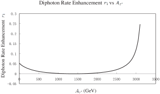
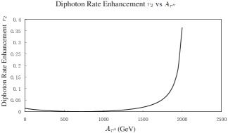
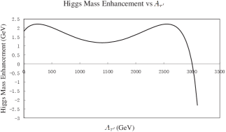
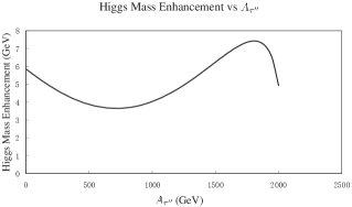
Figure 1: An analysis of the diphoton rate enhancement (top panels) and enhancement of the Higgs boson mass (bottom panels) for the case when the vector masses vanish, i.e., $M_{L}=M_{E}=0$. Left top: A plot of the diphoton rate enhancement $r_{1}$ (from $\tilde{\tau}^{\prime}_{1,2}$) vs $A_{\tau^{\prime}}$; Right top: A plot of the diphoton rate enhancement $r_{2}$ (from $\tilde{\tau}^{\prime\prime}_{1,2}$) vs $A_{\tau^{\prime\prime}}$. Left bottom: A plot of the Higgs mass enhancement from $\hat{\tau}^{\prime}$ sector (GeV) vs $A_{\tau^{\prime}}$; Right bottom: A plot of the Higgs mass enhancement from $\hat{\tau}^{\prime\prime}$ sector (GeV) vs $A_{\tau^{\prime\prime}}$.

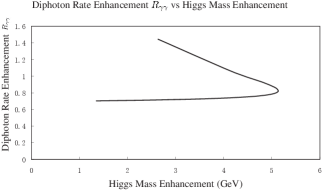
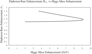
Figure 2: Left panel: A display of the correlation between the Higgs diphoton rate enhancement and the Higgs mass enhancement in the decoupled limit where $M_{L}=M_{E}=0$ as in Fig. 1. Right panel: A display of the correlation between the Higgs diphoton rate enhancement and the Higgs mass enhancement for the case when the vector masses are non-vanishing where $M_{L}=M_{E}=210~{}\mathrm{GeV}$. The two branches shown in each of the two plots are due to the rise and fall of the Higgs mass enhancement as exhibited in the lower panel of Fig. 1 and 3.

Before carrying out the numerical analysis let us summarize the results of the analysis given in Section 4 and Section 5. In Section 4 the correction to the Higgs diphoton rate from the fermionic sector $r_{f}$ was computed in Eq. (21), and the correction from the bosonic sector $r_{b}$ was computed in Eq. (29), while total diphoton rate enhancement $R_{\gamma\gamma}$ is given in Eq. 34. The Higgs boson mass enhancement from the exchange of the vector-like supermultiplets is given in Section 5 where the bosonic contribution is given by Eqs. (39)-(41) and (44)-(46) while the fermionic contribution is given by Eqs. (49)-(51). In this section, for the numerical analysis we impose the constraint that the masses of the new particles be consistent with the experimental lower limits [78].

First, we discuss the decoupled limit where $M_{L}=M_{E}=0$. In this case, both the fermionic sector and the bosonic sector of the vector-like supermultiplets are totally decoupled, and we label the two sectors as the $\hat{\tau}^{\prime}$ and $\hat{\tau}^{\prime\prime}$ sectors, where $\hat{\tau}^{\prime}$ denotes contributions from both $\tau^{\prime}$ and its super-partners $\tilde{\tau}^{\prime}_{1,2}$, and similar for $\hat{\tau}^{\prime\prime}$. Here we choose the following parameters: $M_{1}=M_{2}=500~{}\mathrm{GeV},\,\mu=1~{}\mathrm{TeV},\,\tan\beta=1.4,\,\alpha=\beta-\pi/2,\,y=y^{\prime}=1$ and $m_{h}^{\rm MSSM}=120~{}\mathrm{GeV}$. Using the above parameters and Eq. (21) we find that the fermionic contribution to the Higgs diphoton rate $r_{f}$ is roughly $-0.4$ in this case, which is a large negative effect. However, this is compensated by the contribution from the bosonic sector and this contribution is displayed in the upper two panels of Fig. 1. The upper left panel displays the diphoton rate enhancements from the exchange of $\tilde{\tau}^{\prime}_{1,2}$ in the loop versus $A_{\tau^{\prime}}$ while the upper right panel displays the diphoton rate enhancement from the exchange of $\tilde{\tau}^{\prime\prime}_{1,2}$ versus $A_{\tau^{\prime\prime}}$. As expected in each case we find that the contribution from scalar loops enhances the diphoton rate. The total contribution arising from the sum of the fermionic and the bosonic sectors will be given when we discuss Fig. 2.

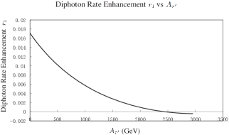
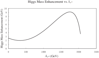
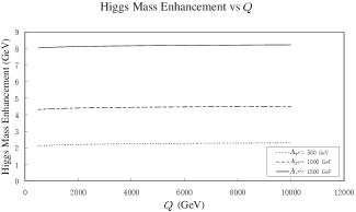
Figure 3: An analysis of the diphoton rate enhancement (top panels) and enhancement of the Higgs boson mass (bottom panels) for the case when the vector masses are non-vanishing where $M_{L}=M_{E}=210~{}\mathrm{GeV}$. Left top: A plot of the Higgs diphoton rate enhancement $r_{1}$ (from $\tilde{\tau}^{\prime}_{1,2}$) vs $A_{\tau^{\prime}}$; Right top: A plot of the Higgs diphoton rate enhancement $r_{2}$ (from $\tilde{\tau}^{\prime\prime}_{1,2}$) vs $A_{\tau^{\prime\prime}}$. Left bottom: A plot of the total Higgs mass enhancement vs $A_{\tau^{\prime\prime}}$; Right bottom: A plot of the total Higgs mass enhancement vs the renormalization group scale $Q$. The three horizontal lines correspond to values of $A_{\tilde{\tau}^{\prime\prime}}=500~{}\mathrm{GeV}$ (bottom), $1000~{}\mathrm{GeV}$ (middle), $1500~{}\mathrm{GeV}$ (top).

An analysis of the enhancement of the Higgs boson mass in the decoupled case ($M_{L}=M_{E}=0$) is given in the lower two panels of Fig. 1. The lower left panel of Fig. 1 gives a display of the Higgs mass enhancement from the exchange of $\hat{\tau}^{\prime}$ sector (including bosonic and fermionic contributions) in the loop versus $A_{\tau^{\prime}}$. Here the contribution to the Higgs boson mass is rather modest not exceeding much beyond 2 GeV over the entire range of $A_{\tau^{\prime}}$. A similar analysis for the mirror sector ($\hat{\tau}^{\prime\prime}$) is given in the right panel of Fig. 1 where the Higgs boson mass enhancement is plotted against $A_{\tau^{\prime\prime}}$. Here large contributions are seen to arise. We turn now to a display of the combined diphoton rate from the fermionic and the bosonic sector versus the combined Higgs boson mass enhancement from the fermionic and bosonic sectors. This analysis is presented in the left panel of Fig. 2 where we display the total diphoton rate enhancement $R_{\gamma\gamma}$ as defined in Eq. (34) versus the total Higgs mass correction (here we chose the maximum value for diphoton rate enhancement from $\tilde{\tau}^{\prime}$ sector, which corresponds to $A_{\tau^{\prime}}=3100~{}\mathrm{GeV}$). While a simultaneous enhancement in both sector does occur, one finds in this case the sizes are rather modest, e.g., one has a 3-4 GeV enhancement in the Higgs boson mass with a 30% enhancement in the diphoton rate at the same time.

Next we discuss the case when $M_{L},M_{E}$ are non-vanishing. Here we choose the following parameters: $M_{L}=M_{E}=210~{}\mathrm{GeV},\,M_{1}=M_{2}=600~{}\mathrm{GeV},\,Q=\mu=1~{}\mathrm{TeV},\,\tan\beta=3,\,\alpha=\beta-\pi/2,\,y=y^{\prime}=1$, and $m_{h}^{\rm MSSM}=120~{}\mathrm{GeV}$. This time, the contribution to the diphoton rate from the fermionic sector is positive and gives $r_{f}\approx+0.1$ on using Eq. (21). The bosonic contribution is exhibited in the upper two panels of Fig. 3, where the upper left panel displays the contribution from the exchange of $\tilde{\tau}^{\prime}_{1,2}$ in the loop versus $A_{\tau^{\prime}}$ while the upper right panel displays the contribution from the exchange of $\tilde{\tau}^{\prime\prime}_{1,2}$ in the loop versus $A_{\tau^{\prime\prime}}$. Here essentially all of the bosonic sector enhancement comes from the $\tau^{\prime\prime}$ sector.

In the lower left panel of Fig. 3 we display the total Higgs mass enhancements (adding up both the bosonic and fermionic contributions) versus $A_{\tau^{\prime\prime}}$, where we choose $A_{\tau^{\prime}}=1000~{}\mathrm{GeV}$. Similar to the diphoton enhancement, the major contribution to the Higgs boson mass enhancement is also from the exchange of $\tilde{\tau}^{\prime\prime}_{1,2}$. In the lower right panel of Fig. 3, we display the total Higgs mass enhancement versus the renormalization group scale $Q$. Again we choose $A_{\tau^{\prime}}=1000~{}\mathrm{GeV}$, and three specific values for $A_{\tau^{\prime\prime}}$ which correspond to three different values of the Higgs mass enhancement, are chosen as shown in the plot. The values for the scale $Q$ cover a large range from 500 GeV to 10 TeV, and we see three almost straight horizontal lines for the Higgs mass enhancement as a function of $Q$. This plot shows the Higgs mass enhancement has almost no dependence on the scale $Q$, which verifies that our approximation in computing the bosonic contribution to the Higgs mass is valid. Combining the diphoton rate from both the bosonic and the fermionic sectors of the vector-like supermultiplets, we display in the right panel of Fig. 2 the total diphoton rate enhancement $R_{\gamma\gamma}$ versus the total Higgs mass correction (where again we fix the contribution from $\tilde{\tau}^{\prime}_{1,2}$ choosing $A_{\tau^{\prime}}=1000~{}\mathrm{GeV}$). Here we find that including the vector masses, one can easily achieve a diphoton rate enhancement as well as a Higgs mass enhancement of substantial size. In Fig. 4 we give a display of the slepton masses. Here one finds that the slepton masses from the new sector are typically in the few hundred GeV range except near the end points and lie substantially above the experimental lower limits [78]. These mass ranges are consistent with the electroweak constraints which have been discussed in a number of works [67, 65, 66, 28, 50, 27].

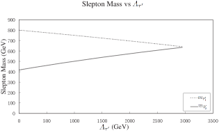
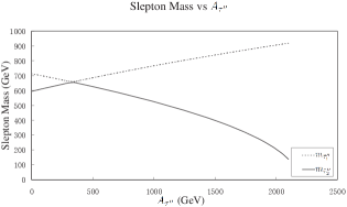
Figure 4: A display of the slepton masses versus the trilinear couplings in the case $M_{L}=M_{E}=210~{}\mathrm{GeV}$. Left panel: A plot of the $\tilde{\tau}^{\prime}_{1,2}$ masses vs $A_{\tau^{\prime}}$. Right panel: A plot of $\tilde{\tau}^{\prime\prime}_{1,2}$ masses vs $A_{\tau^{\prime\prime}}$. We note that the slepton masses over most of the parameter space lie significantly above the experimental lower limits [78].

Finally, we comment on the vacuum stability constraints. These constraints on the $\hat{\tau}^{\prime}$ and $\hat{\tau}^{\prime\prime}$ sectors are similar to those discussed for the stau sector of MSSM and arise from the left-right mixing of the staus [56, 57, 58]. The mixings lead to a cubic term in the Higgs potential expanded around the electroweak symmetry breaking vacuum which is of type $-y\mu h\tilde{\tau}^{\prime}_{L}\tilde{\tau}^{\prime}_{R}$ and $-y^{\prime}\mu h\tilde{\tau}^{\prime\prime}_{L}\tilde{\tau}^{\prime\prime}_{R}$. Such terms can generate global minima in some cases. The parameter that controls the instability is $\mu\tan\beta$. Without going into details because of the smallness of $\mu\tan\beta$ for the analysis given in Figs. 1-4 the solutions we present are consistent with the vacuum stability constraints.

7 Conclusion

In this work we consider an extension of MSSM with vector-like leptonic supermultiplets and its possible implications to the Higgs diphoton rate and to the Higgs boson mass. Specifically we compute one-loop corrections to the diphoton rate of the Higgs boson via the exchange of the new leptons and their super-partners as well as their mirrors. A similar analysis is carried out for the Higgs boson mass where we compute corrections to its mass using the renormalization group improved Coleman-Weinberg effective potential with contributions arising also from these new particles. It is found that an enhancement of the diphoton rate as large as 1.8 can occur and simultaneously a positive correction of 4-10 GeV to the Higgs boson mass can also be obtained due to the exchange of the vector-like supermultiplets. A correction of this size can have a significant effect in relieving the constraint on the weak scale supersymmetry.

In the supergravity unified model with universal boundary conditions at the GUT scale, one finds that for a Higgs mass in the 125-126 GeV region, the squark masses are rather heavy (see Fig. 1 of [13]) and would be difficult to access at the LHC. However, a 5-10 GeV contribution to the Higgs mass from the new sector would put the MSSM component of the Higgs mass in the 116-120 GeV range which allows a significantly lowering of the universal scalar mass (see Fig. 1 of [13]). Thus a Higgs mass correction of the size discussed in this work not only gives a significant correction to the diphoton rate but also lowers the scale of supersymmetry, making sparticles more accessible in the next round of experiments at the LHC [79]. We also note that in the right panel of Fig. 4 one finds that one of the scalar mass eigenvalue can lie close to the current experimental lower limit and thus such states could be accessible at the LHC and at the ILC.

The vector-like leptons can be produced at the LHC via processes such as $pp\to Z\to\tau^{\prime}\bar{\tau}^{\prime}$. The charged vector-like leptons will likely decay inside the detector via their gauge interactions similar to any heavy lepton, e.g., $\tau^{\prime}\to\tau\nu_{\tau^{\prime}}\bar{\nu}_{\tau}$ with the subsequent decay of the $\nu_{\tau^{\prime}}$. The decay of $\nu_{\tau^{\prime}}$ would depend on mixings and is model dependent but in the end it could produce $l^{+}l^{-}\nu_{\tau}$. In this case we have as many as three charged leptons and missing $E_{T}$. However, an accurate analysis of the background is needed to quantify the size of the signal which is outside the scope of this work. Of course the best chance of seeing these particles would be at the ILC through the process $e^{+}e^{-}\to Z\to\tau^{\prime}\bar{\tau}^{\prime}$ if sufficient center of mass energy can be managed.

Acknowledgments: WZF is grateful to HaiPeng An and Tao Liu for helpful discussions. The work of PN is supported in part by the U.S. National Science Foundation (NSF) grants PHY-0757959 and PHY-070467. WZF is supported by funds from The Hong Kong University of Science and Technology.

Appendix A Loop functions

The loop functions $A_{1}(x),A_{\frac{1}{2}}(x)$ and $A_{0}(x)$ that appear in Section 2 are defined by

$$A_{1}(\tau) =-[2+3\tau+3\tau(2-\tau)f(\tau)]\,,$$ (62)

$$A_{\frac{1}{2}}(\tau) =2\tau[1+(1-\tau)f(\tau)]\,,$$ (63)

$$A_{0}(\tau) =-\tau[1-\tau f(\tau)]\,.$$ (64)

Here the function $f(\tau)$ is defined by

$$f(\tau)=\left\{\begin{aligned} &\Big{(}\arcsin\frac{1}{\sqrt{\tau}}\Big{)}^{2}\,,\qquad\tau\geq 1\,;\\ &-\frac{1}{4}\Big{[}\ln\frac{\eta_{+}}{\eta_{-}}-i\pi\Big{]}^{2}\,,\qquad\tau<1\,.\end{aligned}\right.$$ (65)

where $\eta_{\pm}\equiv(1\pm\sqrt{1-\tau})$ and $\tau=4m^{2}\big{/}m_{h}^{2}$ for a particle running in the loop with mass $m$. For the case when $\tau\gg 1$ one has

$$f(\tau)\to\frac{1}{\tau}(1+\frac{1}{3\tau}+\frac{3}{20\tau^{2}}+\cdots)\,,$$ (66)

and in this limit $A_{1}\to-7,\,A_{\frac{1}{2}}\to 4/3,\,A_{0}\to 1/3$.

Appendix B Loop corrections to the Higgs boson mass

In this Appendix we give details of the computation of corrections to the Higgs boson mass-squared matrix arising from radiative corrections to the Higgs boson potential. The Higgs potential is given by

$$V(H_{u},H_{d})=V_{0}+\Delta V\,,$$ (67)

where $V_{0}$ is renormalization group improved tree-level potential and $\Delta V$ is the loop correction. For the case of two Higgs doublets in MSSM, including soft terms the Higgs potential $V$ is given by

$$V_{0} =\overline{m}_{H_{u}}^{2}|H_{u}|^{2}+\overline{m}_{H_{d}}^{2}|H_{d}|^{2}+(|B\mu|^{2}H_{u}.H_{d}+h.c.)+\frac{(g_{2}^{2}-g_{1}^{2})}{4}|H_{u}|^{2}|H_{d}|^{2}$$

$$+\frac{(g_{2}^{2}+g_{1}^{2})}{8}|H_{u}|^{4}+\frac{(g_{2}^{2}+g_{1}^{2})}{8}|H_{d}|^{4}-\frac{g_{2}^{2}}{2}|H_{u}.H_{d}|^{2}\,,$$ (68)

where $\overline{m}_{H_{u}}^{2}=M_{H_{u}}^{2}+|\mu|^{2},\,\overline{m}_{H_{d}}^{2}=M_{H_{d}}^{2}+|\mu|^{2}$, and $M_{H_{u,d}}$ and $B$ are the soft parameters. The correction $\Delta V$ to the effective potential at the one loop level is given by [76, 77]

$$\Delta V=\frac{1}{64\pi^{2}}Str\Big{[}M^{4}_{i}(H_{u},H_{d})\Big{(}\ln\frac{M^{2}_{i}(H_{u},H_{d})}{Q^{2}}-\frac{3}{2}\Big{)}\Big{]}\,,$$ (69)

where $M_{i}$ is the mass eigenvalue of the particle being exchanged, $Str$ stands for the sum $\sum_{i}c_{i}(2J_{i}+1)(-1)^{2J_{i}}$, $c_{i}(2J_{i}+1)$ counts the degrees of freedom, and the sum runs over all the particles $i$ bosonic and fermionic being exchange in the loop. Thus to construct the mass-squared matrix of the Higgs scalars we need to compute the quantity

$$(M_{H})^{2}_{\alpha\beta}=\frac{\partial^{2}V}{\partial v_{\alpha}\partial v_{\beta}}=(M_{H}^{2})^{0}_{\alpha\beta}+\Delta M^{2}_{H\alpha\beta}\,,$$ (70)

where $(\alpha,\beta)=(1,2)$ and $v_{1}\equiv v_{d},~{}v_{2}\equiv v_{u}$; $(M_{H}^{2})_{\alpha\beta}^{0}$ is the contribution from $V_{0}$ and $\Delta M^{2}_{H\alpha\beta}$ is the contribution from $\Delta V$. $\Delta M^{2}_{H\alpha\beta}$ is given by

$$\Delta M^{2}_{H\alpha\beta}=\frac{1}{32\pi^{2}}Str\Big{[}\frac{\partial M_{i}^{2}}{\partial v_{\alpha}}\frac{\partial M_{i}^{2}}{\partial v_{\beta}}\ln\frac{M_{i}^{2}}{Q^{2}}+M_{i}^{2}\frac{\partial^{2}M_{i}^{2}}{\partial v_{\alpha}\partial v_{\beta}}\Big{(}\ln\frac{M_{i}^{2}}{Q^{2}}-1\Big{)}\Big{]}\,.$$ (71)

In the analysis of corrections to the Higgs boson mass the variations with respect to the fields $v_{u},v_{d}$ play an important role. Thus variations with respect to $v_{u}$ and $v_{d}$ give the following two constraints

$$\overline{m}_{H_{d}}^{2}+\frac{g_{2}^{2}+g_{1}^{2}}{8}(v_{d}^{2}-v_{u}^{2})+|B\mu|^{2}\tan\beta+\frac{1}{v_{d}}\frac{\partial\Delta V}{\partial v_{d}} =0\,,$$ (72)

$$\overline{m}_{H_{u}}^{2}-\frac{g_{2}^{2}+g_{1}^{2}}{8}(v_{d}^{2}-v_{u}^{2})+|B\mu|^{2}\cot\beta+\frac{1}{v_{u}}\frac{\partial\Delta V}{\partial v_{u}} =0\,.$$ (73)

In the computation of the Higgs boson mass-squared matrix it is found convenient to eliminate $\overline{m}_{H_{u}}^{2}$ and $\overline{m}_{H_{d}}^{2}$ using the constraints of Eqs. (72) and (73). This allows us to write

$$M_{H}^{2}=\left(\begin{matrix}M_{Z}^{2}c_{\beta}^{2}+M_{A}^{2}s_{\beta}^{2}+\Delta_{11}&-(M_{Z}^{2}+M_{A}^{2})s_{\beta}c_{\beta}+\Delta_{12}\cr-(M_{Z}^{2}+M_{A}^{2})s_{\beta}c_{\beta}+\Delta_{12}&M_{Z}^{2}s_{\beta}^{2}+M_{A}^{2}c_{\beta}^{2}+\Delta_{22}\end{matrix}\right)\,,$$ (74)

where $M_{Z}^{2}=\frac{1}{4}(g_{1}^{2}+g_{2}^{2})(v_{u}^{2}+v_{d}^{2})$ and $M_{A}^{2}=-2|B\mu|^{2}\big{/}\sin(2\beta)+\cdots$ and $\Delta_{ij}$ are now given by [74, 75]:

$$\Delta_{11} =\Big{(}-\frac{1}{v_{d}}\frac{\partial}{\partial v_{d}}+\frac{\partial^{2}}{\partial v_{d}^{2}}\Big{)}\Delta V\,,$$ (75)

$$\Delta_{22} =\Big{(}-\frac{1}{v_{u}}\frac{\partial}{\partial v_{u}}+\frac{\partial^{2}}{\partial v_{u}^{2}}\Big{)}\Delta V\,,$$ (76)

$$\Delta_{12} =\frac{\partial^{2}}{\partial v_{u}\partial v_{d}}\Delta V\,.$$ (77)

Evaluations of $\Delta_{ij}$ for the vector-like leptonic supermultiplet are given in Section 5.