Quantum Monte Carlo study of nonequilibrium transport through a quantum dot coupled to normal and superconducting leads

Abstract

We investigate the nonequilibrium phenomena through the quantum dot coupled to the normal and superconducting leads using a weak-coupling continuous-time Monte Carlo method. Calculating the time evolution of particle number, double occupancy, and pairing correlation at the quantum dot, we discuss how the system approaches the steady state. We also deduce the steady current through the quantum dot beyond the linear response region. It is clarified that the interaction decreases the current in the Kondo-singlet dominant region. On the other hand, when the quantum dot is tightly coupled to the superconducting lead, the current is increased by the introduction of the Coulomb interaction, which originates from the competition between the Kondo and proximity effects. Transient currents induced by the interaction quench are also addressed.

I Introduction

Recently electron transport through nanofabrications has attracted much interest. One of the simplest systems is a quantum dot with discrete energy levels,dot which gives us a stage to study fundamental quantum physics. When the quantum dot is contacted with the normal leads, electron correlations play a crucial role in understanding its transport at low temperatures where the Coulomb blockade and Kondo effect appear. On the other hand, when superconducting leads are connected to the quantum dot,dotS the proximity-induced on-dot pairing becomes important, in addition to electron correlations. However, multiple Andreev reflections should dominate the system and it is difficult to study the interplay between the superconducting and electron correlations systematically.

The quantum dot system coupled to the normal and superconducting leads is one of the appropriate systems to study how the transport properties are affected by the competition between the Kondo and proximity-induced on-dot pairing effects. In fact, the system has experimentally been examined, Graber ; Hofstetter ; Herrmann and the Kondo-enhanced Andreev transport has recently been observed in the InAs quantum dot.Deacon ; Deacon2 Theoretical study has been done by many groups, slave1 ; slave2 ; Domanski ; nca ; Cuevas ; Yamada ; Tanaka ; Baranski ; Koerting and some interesting transport properties have successfully been explained. However, it is nontrivial how the techniques are applicable in the strong coupling and high voltage region. This may be important to understand the experimental results quantitatively since the linear response region is narrow in the quantum dot system. Therefore, the unbiased and robust method for the nonequilibrium phenomena is desired.

To this end, we make use of the continuous-time quantum Monte Carlo (CTQMC) method CTQMC based on the Keldysh formalism. WernerOka ; Werner Here we extend the CTQMC method in the continuous-time auxiliary field (CTAUX) formulation Gull to treat the superconducting state in the Nambu formalism. Calculating the particle number, double occupancy, pairing correlations and current through the quantum dot, we study the nonequilibrium phenomena. We also discuss the competition between the Kondo and proximity effects on the steady-state in the quantum dot coupled to the normal and superconducting leads.

The paper is organized as follows. In Sec. II, we introduce the model Hamiltonian for the quantum dot coupled to the normal and superconducting leads. The CTQMC algorithm in the Nambu formalism is explained in Sec. III. In Sec. IV, we discuss the nonequilibrium phenomena in the quantum dot system. A brief summary is given in Sec. V.

II Model

We consider the electron transport through the quantum dot coupled to the normal and superconducting leads, which are labeled by $\alpha=N$ and $S$. For simplicity, we use a single level quantum dot with the Coulomb interaction. The system should be described by the following Anderson impurity Hamiltonian as

$$H = H_{bath}+H_{hyb}+H_{dot},$$ (1)

$$H_{bath} = \sum_{k\alpha\sigma}\left(\epsilon_{k\alpha}-\mu_{\alpha}\right)c_{k\alpha\sigma}^{\dagger}c_{k\alpha\sigma}$$ (2)

$$+ \sum_{k}\left(\Delta_{S}c_{-kS\downarrow}^{\dagger}c_{kS\uparrow}^{\dagger}+\Delta_{S}^{*}c_{kS\uparrow}c_{-kS\downarrow}\right),$$

$$H_{hyb} = \sum_{k\alpha\sigma}\left(V_{k\alpha}c_{k\alpha\sigma}^{\dagger}d_{\sigma}+V_{k\alpha}^{*}d_{\sigma}^{\dagger}c_{k\alpha\sigma}\right),$$ (3)

$$H_{dot} = H_{dot}^{0}+H^{\prime},$$ (4)

$$H_{dot}^{0} = \sum_{\sigma}\left(\epsilon_{d}+\frac{U}{2}\right)n_{\sigma},$$ (5)

$$H^{\prime} = U\left(n_{\uparrow}n_{\downarrow}-\frac{1}{2}\sum_{\sigma}n_{\sigma}\right),$$ (6)

where $c_{k\alpha\sigma}(c_{k\alpha\sigma}^{\dagger})$ is the annihilation (creation) operator of an electron with wave vector $k$ and spin $\sigma(=\uparrow,\downarrow)$ in the $\alpha$th lead. $d_{\sigma}(d_{\sigma}^{\dagger})$ is the annihilation (creation) operator of an electron at the quantum dot and $n_{\sigma}=d_{\sigma}^{\dagger}d_{\sigma}$. $\epsilon_{k\alpha}$ is the dispersion relation of the $\alpha$th lead and $V_{k\alpha}$ is the hybridization between the $\alpha$th lead and the quantum dot. $\epsilon_{d}$ and $U$ is the energy level and the Coulomb interaction at the quantum dot. To discuss the nonequilibrium state in the system, we set the chemical potential in each lead as $\mu_{N}=V$ and $\mu_{S}=0$, where $V$ is the bias voltage. In our paper, we focus on the particle-hole symmetric system with $\epsilon_{d}+U/2=0$ and the superconducting lead is assumed to be described by the BCS theory with an isotropic gap $\Delta_{S}=\Delta(>0)$. We consider a sufficiently wide bandwidth in both leads, where the coupling strength $\Gamma_{\alpha}(\omega)=\pi\sum_{k}\left|V_{k\alpha}\right|^{2}\delta(\omega-\epsilon_{k\alpha})$ becomes constant.

When no bias voltage is applied to the system, ground state properties depend on the ratio $\Gamma_{S}/\Gamma_{N}$. In the case $\Gamma_{S}/\Gamma_{N}\ll 1$ and $U\neq 0$, conduction electrons in the normal lead screen the local spin at the quantum dot and the Kondo-singlet dominant state is realized. On the other hand, the singlet Cooper pairs are realized at a quantum dot due to the proximity effect when $\Gamma_{S}/\Gamma_{N}\gg 1$. It is known that when the ratio is changed, the crossover, in general, occurs between these two singlet states and the first-order transition occurs in the limit $\Gamma_{N}=0$. Yamada ; Koerting ; Satori

This crossover affects nonequilibrium properties in the quantum dot system. It has been reported how the zero bias conductanceCuevas ; Tanaka and the current-voltage characteristicsKoerting are affected in the vicinity of the crossover. Furthermore, a detailed structure in the differential conductance has been discussed in the nonlinear response region by means of the modified perturbation theory (MPT),Yamada which is based on an interpolation scheme between the weak-coupling limit $(U\rightarrow 0)$ and the superconducting atomic limit $(\Gamma_{N}=0$, $\Delta\rightarrow\infty$). Although the reliable results have been obtained in the cases $U/\Gamma_{N}\ll 1$ and $\Gamma_{S}/\Gamma_{N}\gg 1$, it is unclear whether the nonlinear response in the strong coupling region is quantitatively described or not.

In this paper, we make use of the CTQMC method. In the method, Monte Carlo samplings of collections of diagrams are performed in continuous time and thereby the Trotter error, which originates from the Suzuki-Trotter decomposition, is avoided. This method has successfully been applied to many equilibrium systems. Recently, the CTQMC method based on the Keldysh formalism has been formulated, where the nonequilibrium phenomena in the quantum dot coupled to normal leads have quantitatively been studied.WernerOka ; Werner In the following, we extend the CTQMC method to deal with the superconducting state in the Nambu formalism.

III Continuous-Time Quantum Monte Carlo Simulations in the Nambu Formalism

In this section, we explain the CTQMC method based on the Keldysh formalism,WernerOka ; Werner and extend it to treat the superconducting state. Here, we consider a weak-coupling version of the CTQMC approach. Since the interaction is considered as a perturbation, we can examine the time evolution of the system after the interaction quench. We start with the following identity

$$1 = {\rm Tr}\left[\rho_{0}e^{it\left(H_{0}+H^{\prime}-K/t\right)}e^{-it\left(H_{0}+H^{\prime}-K/t\right)}\right],$$ (7)

where $\rho_{0}(=e^{-\beta H_{0}}/{\rm Tr}e^{-\beta H_{0}})$ is the initial density matrix for $H_{0}(=H-H^{\prime})$ and $K$ is some nonzero constant. It is then given by

$$1 = {\rm Tr}\Big{\{}\rho_{0}\tilde{T}\left[\exp\Big{\{}i\int_{0}^{t}d\tilde{t}\left(H^{\prime}(\tilde{t})-K/t\right)\Big{\}}\right]e^{itH_{0}}$$

$$\times e^{-itH_{0}}T\left[\exp\Big{\{}-i\int_{0}^{t}dt\left(H^{\prime}(t)-K/t\right)\Big{\}}\right]\Big{\}},$$

where $O(t)=e^{itH_{0}}Oe^{-itH_{0}}$ is the interaction representation of the operator $O$ and $T(\tilde{T})$ is the time-ordering (antitime-ordering) operator. Expanding the exponentials into a power series, we obtain

$$1 = {\rm Tr}\Big{[}\rho_{0}\sum_{l}(-\frac{iK}{t})^{l}\int_{0}^{t}d\tilde{t}_{1}\cdots\int_{\tilde{t}_{l-1}}^{t}d\tilde{t}_{l}e^{i\tilde{t}_{1}H_{0}}$$ (8)

$$\times (1-\frac{t}{K}H^{\prime})\cdots e^{i(\tilde{t}_{l}-\tilde{t}_{l-1})H_{0}}(1-\frac{t}{K}H^{\prime})e^{i(t-\tilde{t}_{l})H_{0}}$$

$$\times \sum_{m}(\frac{iK}{t})^{m}\int_{0}^{t}dt_{1}\cdots\int_{t_{m-1}}^{t}dt_{m}e^{-i(t-t_{m})H_{0}}$$

$$\times (1-\frac{t}{K}H^{\prime})\cdots e^{-i(t_{2}-t_{1})H_{0}}(1-\frac{t}{K}H^{\prime})e^{-it_{1}H_{0}}\Big{]}$$

$$= \frac{1}{{\rm Tr}\left[e^{-\beta H_{0}}\right]}\sum_{lm}(-i)^{l}i^{m}\left(\frac{K}{2t}\right)^{l+m}\sum_{\{\tilde{s}\}\{s\}}$$

$$\times \int_{0}^{t}d\tilde{t}_{1}\cdots\int_{\tilde{t}_{l-1}}^{t}d\tilde{t}_{l}\int_{0}^{t}dt_{1}\cdots\int_{t_{m-1}}^{t}dt_{m}$$

$$\times {\rm Tr}\Big{[}e^{-\beta H_{0}}e^{i{\tilde{t}}_{1}H_{0}}e^{\gamma\tilde{s}_{1}(n_{\uparrow}-n_{\downarrow})}\cdots e^{i({\tilde{t}}_{l}-{\tilde{t}}_{l-1})H_{0}}$$

$$\times e^{\gamma\tilde{s}_{l}(n_{\uparrow}-n_{\downarrow})}e^{-i({\tilde{t}}_{l}-t_{m})H_{0}}e^{\gamma s_{m}(n_{\uparrow}-n_{\downarrow})}\cdots$$

$$\times e^{-i(t_{2}-t_{1})H_{0}}e^{\gamma s_{1}(n_{\uparrow}-n_{\downarrow})}e^{-it_{1}H_{0}}\Big{]},$$

where we have used the following equation as

$$1-\frac{tU}{K}\left(n_{\uparrow}n_{\downarrow}-\frac{1}{2}\sum_{\sigma}n_{\sigma}\right)=\frac{1}{2}\sum_{s=\pm 1}e^{\gamma s(n_{\uparrow}-n_{\downarrow})}$$ (9)

with $\gamma=\cosh^{-1}(1+tU/2K)$. The introduction of the Ising variable $s$ in $H^{\prime}$ allows us to perform Monte Carlo simulations. An $(l+m)$th order configuration $c=\{s_{k_{1}},s_{k_{2}},\cdots,s_{k_{n}};t_{k_{1}},t_{k_{2}},\cdots,t_{k_{n}}\}$ is represented by the auxiliary spins $s_{k_{1}},s_{k_{2}},\cdots,s_{k_{n}}$ at the Keldysh times $t_{k_{1}},t_{k_{2}},\cdots,t_{k_{n}}$ along the Keldysh contour, where the $l(m)$ denotes the number of spins on the forward (backward) contour (see Fig. 1) and $n=l+m$.

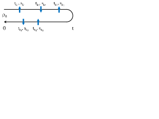
Figure 1: Illustration of the Keldysh contour for the CTQMC method. Arrows represent auxiliary Ising spins for a certain Monte Carlo configuration corresponding to the perturbation order $l=3$ and $m=2$ $(n=5)$.

Its weight $w_{c}$ is then given as

$$w_{c} = (-i)^{l}i^{m}\left(\frac{Kdt}{2t}\right)^{n}\det\left[{\hat{N}}^{(n)}\right]^{-1},$$ (10)

where ${\hat{N}}$ is an $n\times n$ matrix and its element consists of a $2\times 2$ matrix:

$$\begin{array}[]{rcl}\left[{\hat{N}}^{(n)}\right]^{-1}&=&{\hat{\Gamma}}^{(n)}-{\hat{g}}^{(n)}\left({\hat{\Gamma}}^{(n)}-{\hat{I}}^{(n)}\right),\\ {\hat{I}}^{(n)}_{ij}&=&\delta_{ij}{\hat{\sigma}}_{0},\\ {\hat{\Gamma}}^{(n)}_{ij}&=&\delta_{ij}\exp\left({\gamma s_{k_{i}}{\hat{\sigma}}_{z}}\right),\\ {\hat{g}}^{(n)}_{ij}&=&{\hat{\sigma}}_{z}{\hat{G}}_{0}(t_{k_{i}},t_{k_{j}}),\end{array}$$ (11)

with $i,j=1,2,\cdots,n$. The Green’s function is explicitly given by

$$\begin{array}[]{rcl}{\hat{G}}_{0}(t^{\prime}_{k},t^{\prime\prime}_{k})&=&\left\{\begin{array}[]{ll}{\hat{G}}_{0}^{<}(t^{\prime},t^{\prime\prime}),&t^{\prime}_{k}<t^{\prime\prime}_{k}\\ {\hat{G}}_{0}^{>}(t^{\prime},t^{\prime\prime}),&t^{\prime}_{k}\geq t^{\prime\prime}_{k}\end{array}\right.\end{array},$$ (12)

where the times $t^{\prime}$ and $t^{\prime\prime}$ correspond to the Keldysh times $t_{k}^{\prime}$ and $t_{k}^{\prime\prime}$. The lesser and greater Green’s functions are defined by a $2\times 2$ matrix as

$$\begin{array}[]{rcl}{\hat{G}}_{0}^{<}(t^{\prime},t^{\prime\prime})&=&i\left(\begin{array}[]{cc}\langle d_{\uparrow}^{\dagger}(t^{\prime\prime})d_{\uparrow}(t^{\prime})\rangle&\langle d_{\downarrow}(t^{\prime\prime})d_{\uparrow}(t^{\prime})\rangle\\ \langle d_{\uparrow}^{\dagger}(t^{\prime\prime})d_{\downarrow}^{\dagger}(t^{\prime})\rangle&\langle d_{\downarrow}(t^{\prime\prime})d_{\downarrow}^{\dagger}(t^{\prime})\rangle\end{array}\right),\\ {\hat{G}}_{0}^{>}(t^{\prime},t^{\prime\prime})&=&-i\left(\begin{array}[]{cc}\langle d_{\uparrow}(t^{\prime})d_{\uparrow}^{\dagger}(t^{\prime\prime})\rangle&\langle d_{\uparrow}(t^{\prime})d_{\downarrow}(t^{\prime\prime})\rangle\\ \langle d_{\downarrow}^{\dagger}(t^{\prime})d_{\uparrow}^{\dagger}(t^{\prime\prime})\rangle&\langle d_{\downarrow}^{\dagger}(t^{\prime})d_{\downarrow}(t^{\prime\prime})\rangle\end{array}\right).\end{array}$$ (13)

These Green’s functions for the quantum dot system coupled to the normal and superconducting leads have been obtained by the standard technique, Yamada ; Cuevas which are explicitly represented in Appendix A.

The sampling process must satisfy ergodicity and (as a sufficient condition) detailed balance. For ergodicity, it is enough to insert or remove the Ising variables with random orientations at random times to generate all possible configurations. To satisfy the detailed balance condition, we decompose the transition probability as

$$p(i\rightarrow j) = p^{prop}(i\rightarrow j)p^{acc}(i\rightarrow j)$$ (14)

where $p^{prop}(p^{acc})$ is the probability to propose (accept) the transition from the configuration $i$ to the configuration $j$. Here, we consider the insertion and removal of the Ising spins as one step of the simulation process, which corresponds to a change of $\pm 1$ in the perturbation order. The probability of insertion/removal of an Ising spin is then given by

$$p^{prop}(n\rightarrow n+1) = \frac{1}{2}\frac{dt}{2t}$$ (15)

$$p^{prop}(n+1\rightarrow n) = \frac{1}{n+1}.$$ (16)

For this choice, the ratio of the acceptance probabilities becomes

$$\frac{p^{prop}(n\rightarrow n+1)}{p^{prop}(n+1\rightarrow n)} = \pm i\frac{2K}{n+1}\frac{{\rm det}\left[{\hat{N}}^{(n)}\right]}{{\rm det}\left[{\hat{N}}^{(n+1)}\right]},$$ (17)

where $+i(-i)$ corresponding to a spin which is inserted on the forward (backward) contour.

When the Metropolis algorithm is used to sample the configurations, we accept the transition from $n$ to $n\pm 1$ with the probability

$${\rm min}\left[1,\frac{p^{prop}(n\rightarrow n\pm 1)}{p^{prop}(n\pm 1\rightarrow n)}\right].$$ (18)

In each Monte Carlo step, we can measure the Green function ${\hat{G}}(t,t^{\prime})$. By using Wick’s theorem, the contribution of a certain configuration is given by

$$\begin{array}[]{rcl}\displaystyle\hfil&&\frac{\displaystyle w_{G}\Big{\{}\left[(t_{k_{1}},s_{k_{1}}),\cdots,(t_{k_{n}},s_{k_{n}})\right];{\hat{G}}(t^{\prime},t^{\prime\prime})\Big{\}}}{\displaystyle w\Big{\{}\left[(t_{k_{1}},s_{k_{1}}),\cdots,(t_{k_{n}},s_{k_{n}})\right]\Big{\}}}\\ &=&{\rm det}\left[{\hat{N}}^{(n)}\right]{\rm det}\left(\begin{array}[]{cc}\left[{\hat{N}}^{(n)}\right]^{-1}&{\hat{G}}_{0}(t_{k_{i}},t^{\prime\prime})\\ {\hat{G}}_{0}(t^{\prime},t_{k_{j}})(\hat{\Gamma}-\hat{I})&{\hat{G}}_{0}(t^{\prime},t^{\prime\prime})\end{array}\right)\\ &=&\displaystyle{\hat{G}}_{0}(t^{\prime},t^{\prime\prime})\\ &+&\displaystyle i\sum_{ij}{\hat{G}}_{0}(t^{\prime},t_{k_{i}})\left[\left(\hat{\Gamma}-\hat{I}\right)\hat{N}\right]_{ij}{\hat{G}}_{0}(t_{k,j},t^{\prime\prime}).\end{array}$$

The expectation values of the particle number $N(t)=\sum_{\sigma}\langle n_{\sigma}(t)\rangle$, pairing correlations $P(t)=\langle c_{\uparrow}(t)c_{\downarrow}(t)\rangle$, and double occupancy $D(t)=\langle n_{\uparrow}(t)n_{\downarrow}(t)\rangle$ at the quantum dot are calculated as

$$N(t) = 2-i\langle G_{11}(t,t)\rangle+i\langle G_{22}(t,t)\rangle,$$ (19)

$$P(t) = i\langle G_{12}(t,t)\rangle,$$ (20)

$$D(t) = 1-N(t)+\langle{\rm det}{\hat{G}}(t,t)\rangle.$$ (21)

We also measure the current from the quantum dot to the $\alpha$th lead, which is given as

$$I_{\alpha} = -2{\rm Im}\sum_{k\sigma}V_{k\alpha\sigma}\langle c_{k\alpha\sigma}^{\dagger}d_{\sigma}\rangle.$$ (22)

For convenient, we use the composite operator $\tilde{c}_{\alpha\sigma}=\sum_{k}V_{k\alpha\sigma}c_{k\alpha\sigma}$ and consider the following matrix as

$$\begin{array}[]{rcl}{\hat{A}}_{0\alpha}(t^{\prime}_{k},t^{\prime\prime}_{k})&=&\left\{\begin{array}[]{ll}{\hat{A}}_{0\alpha}^{<}(t^{\prime},t^{\prime\prime}),&t^{\prime}_{k}\leq t^{\prime\prime}_{k}\\ {\hat{A}}_{0\alpha}^{>}(t^{\prime},t^{\prime\prime}),&t^{\prime}_{k}>t^{\prime\prime}_{k}\end{array}\right.,\end{array}$$ (23)

where

$$\begin{array}[]{rcl}{\hat{A}}_{0\alpha}^{<}(t^{\prime},t^{\prime\prime})&=&i\left(\begin{array}[]{cc}\langle\tilde{c}_{\alpha\uparrow}^{\dagger}(t^{\prime\prime})d_{\uparrow}(t^{\prime})\rangle&\langle\tilde{c}_{\alpha\downarrow}(t^{\prime\prime})d_{\uparrow}(t^{\prime})\rangle\\ \langle\tilde{c}_{\alpha\uparrow}^{\dagger}(t^{\prime\prime})d_{\downarrow}^{\dagger}(t^{\prime})\rangle&\langle\tilde{c}_{\alpha\downarrow}(t^{\prime\prime})d_{\downarrow}^{\dagger}(t^{\prime})\rangle\end{array}\right),\\ {\hat{A}}_{0\alpha}^{>}(t^{\prime},t^{\prime\prime})&=&-i\left(\begin{array}[]{cc}\langle d_{\uparrow}(t^{\prime})\tilde{c}_{\alpha\uparrow}^{\dagger}(t^{\prime\prime})\rangle&\langle d_{\uparrow}(t^{\prime})\tilde{c}_{\alpha\downarrow}(t^{\prime\prime})\rangle\\ \langle d_{\downarrow}^{\dagger}(t^{\prime})\tilde{c}_{\alpha\uparrow}^{\dagger}(t^{\prime\prime})\rangle&\langle d_{\downarrow}^{\dagger}(t^{\prime})\tilde{c}_{\alpha\downarrow}(t^{\prime\prime})\rangle\end{array}\right).\end{array}$$ (24)

The contribution for the matrix ${\hat{A}}_{0\alpha}(t^{\prime},t^{\prime\prime})$ of a certain configuration is given by

$$\begin{array}[]{rcl}\displaystyle\hfil&&\frac{\displaystyle w_{A}\Big{\{}\left[(t_{k_{1}},s_{k_{1}}),\cdots,(t_{k_{n}},s_{k_{n}})\right];{\hat{A}}_{\alpha}(t^{\prime},t^{\prime\prime})\Big{\}}}{\displaystyle w\Big{\{}\left[(t_{k_{1}},s_{k_{1}}),\cdots,(t_{k_{n}},s_{k_{n}})\right]\Big{\}}}\\ &=&\displaystyle{\rm det}\left[{\hat{N}}^{(n)}\right]{\rm det}\left(\begin{array}[]{cc}\left[{\hat{N}}^{(n)}\right]^{-1}&{\hat{A}}_{0\alpha}(t_{k_{i}},t^{\prime\prime})\\ {\hat{G}}_{0}(t^{\prime},t_{k_{j}})(\hat{\Gamma}-\hat{I})&{\hat{A}}_{0\alpha}(t^{\prime},t^{\prime\prime})\end{array}\right)\\ &=&\displaystyle{\hat{A}}_{0\alpha}(t^{\prime},t^{\prime\prime})\\ &+&\displaystyle i\sum_{ij}{\hat{G}}_{0}(t^{\prime},t_{k_{i}})\left[\left(\hat{\Gamma}-\hat{I}\right)\hat{N}\right]_{ij}{\hat{A}}_{0\alpha}(t_{k_{j}},t^{\prime\prime}).\end{array}$$

Then we obtain the measurement formula for the currents as

$$I_{\alpha}(t) = -2{\rm Im}\Big{[}\langle{\hat{A}}_{\alpha}(t,t)\rangle_{11}-\langle{\hat{A}}_{\alpha}(t,t)\rangle_{22}\Big{]}.$$ (25)

This algorithm is essentially the same as the CTQMC method for the equilibrium state,KogaWerner and thereby it is straightforward to modify the codes to deal with the nonequilibrium system. Here, we comment on the dynamical sign problem: the weight for a certain configuration is, in general, represented by the complex number [see eq. (10)]. As discussed in the previous works,WernerOka ; Werner the dynamical sign problem becomes more serious in the simulations on longer contours and accurate measurements of physical quantities are restricted to a certain time $t_{max}$. The introduction of the coupling strength $\Gamma_{S}$ reduces the sign problem, which allows us to perform the simulations on longer contours. On the other hand, the bias voltage $V$ little affects the dynamical sign problem. Therefore, performing Monte Carlo simulations with a fixed $t_{max}$, we can equally treat the systems with different values of $V$, where the precision of the obtained results little varies. This is contrast to the perturbative approach, where more accurate results should be obtained in the vicinity of $V=0$.

In this study, we use the coupling constant of the normal lead $\Gamma_{N}$ as the unit of energy, and fix the superconducting gap as $\Delta/\Gamma_{N}=0.5$. In the following, we perform the CTQMC simulations to discuss nonequilibrium behavior at zero temperature in the quantum dot coupled to the normal and superconducting leads.

IV Results

In this section, we discuss how the interaction quench affects the time evolution of the physical quantities. Furthermore, by extrapolating them in the $t\rightarrow\infty$ limit, we discuss steady-state properties of the quantum dot system.

First, we consider the quantum dot system without the bias voltage. The time evolutions of the double occupancy and pair correlation are shown in Figs. 2 (a) and (c).

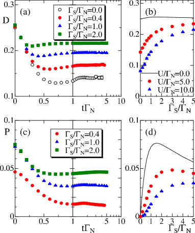
Figure 2: The double occupancy (upper panels) and pairing correlation (lower panels) in the system with $T=0$, $V=0$, $\Delta/\Gamma_{N}=0.5$ and $\epsilon_{d}+U/2=0$. The time evolutions are shown in (a) and (c), and the quantities at the steady state are shown in (b) and (d).

In these figures, the quantities are shown on the linear plot in the initial relaxation region $(t\Gamma_{N}<1)$ and on the logarithmic plot in the rest $(t\Gamma_{N}>1)$. When $\Gamma_{S}=0$, the quantum dot is only coupled to the normal lead and the system is reduced to the conventional Anderson impurity model, where our results reproduce the previous ones. WernerOka We find that the interaction quench decreases the double occupancy ($t\Gamma_{N}<1)$ and the system approaches the steady state $(t\Gamma_{N}>2)$. When the superconducting lead couples to the quantum dot, the double occupancy and pairing correlation for the initial state $(t\leq 0)$ increase due to the proximity effect. As the interaction is turned on at $t=0$, the double occupancy slightly decreases and the system quickly approaches the steady state, by comparing with the case $\Gamma_{S}=0$, as seen in Fig. 2 (a). This implies that electron correlations become less important in the system. Although $t_{max}$ is finite, two quantities seem to converge around $t=t_{max}$. This allows us to discuss the steady-state properties in the system.

Regarding the physical quantities at $t=t_{max}$ as those for the steady state, we discuss the ground state properties. The results are shown in Figs. 2 (b) and (d). When the quantum dot is only contacted to the normal lead $(\Gamma_{S}=0)$, the Coulomb interaction decreases the double occupancy and the Kondo-singlet dominant state is realized. As the coupling strength $\Gamma_{S}$ increases, the double occupancy $D$ and pair correlation $P$ increase due to the proximity effect. In the large $\Gamma_{S}$ region, the proximity-induced on-dot singlet-pairing dominant state is realized and electron correlations become irrelevant. In fact, the double occupancy approaches the value in the noninteracting limit $(D\rightarrow 1/4)$. Therefore, the crossover occurs between the Kondo-singlet and proximity-induced singlet-pairing dominant states.Yamada

When the bias voltage is applied, the current begins to flow between leads. In the steady state $(t\rightarrow\infty)$, the current $I$ through the quantum dot is constant ($I=I_{N}=-I_{S}$). In the transient regime, the current from the dot to the $\alpha$th lead is affected by the interaction $U$ and hybridization $\Gamma_{\alpha}$, which results in different values at a certain time $t$. Therefore, we calculate both currents independently. The results for $\Gamma_{S}/\Gamma_{N}=1$ are shown in Fig. 3.

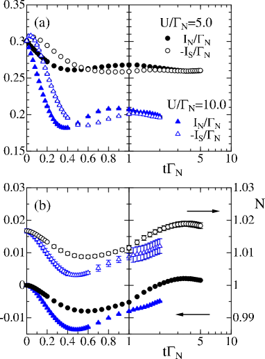
Figure 3: The results are obtained by the CTQMC method in the quantum dot system with $\Gamma_{S}/\Gamma_{N}=1$, $V/\Gamma_{N}=0.5$, $\Delta/\Gamma_{N}=0.5$ and $T=0$ when $U/\Gamma_{N}=5.0$ (circles) and $U/\Gamma_{N}=10.0$ (triangles). (a) Solid (open) symbols represent the time evolution of the current $I_{N}\;(-I_{S})$. (b) Solid (open) symbols represent the integrated total currents $\sum_{\alpha}\int_{0}^{t}I_{\alpha}(t^{\prime})dt^{\prime}$ and particle number $N(t)$ at the quantum dot.

In the initial state $(t\leq 0)$, the currents $I_{\alpha}$ are given by the steady current through the noninteracting dot. The introduction of the interaction decreases the currents $|I_{N}|$ and $|I_{S}|$ differently, and oscillation behavior appears, as shown in Fig. 3 (a). Finally, $I_{N}\sim-I_{S}$ and the system approaches the steady state. We note that the steady current can be extrapolated since the relaxation of oscillation behavior appears in the transient current.

Here, we check the law of conservation of charge, which should be described as

$$\sum_{\alpha}\int_{0}^{t}I_{\alpha}(t^{\prime})dt^{\prime}=N(t)-N(0).$$ (26)

Fig. 3 (b) shows the integrated total currents from the quantum dot [left-hand side of eq. (26)] and particle number at the quantum dot $N(t)$. It is found that the difference of two quantities is always constant, which means that the conservation law, eq. (26), is satisfied within our numerical accuracy. This relation provides a good check for the numerical implementation.

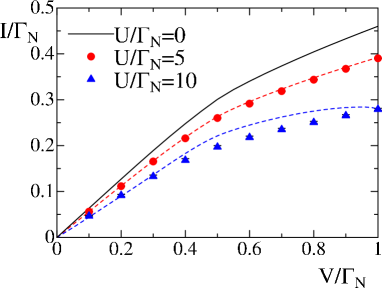
Figure 4: Current-voltage characteristics in the system with $\Gamma_{S}/\Gamma_{N}=1$, $\Delta/\Gamma_{N}=0.5$, and $T=0$. Circles and triangles represent the CTQMC results for $U/\Gamma_{N}=5.0$ and $10.0$ at $t=t_{max}$. Dashed lines represent the MPT results at the low temperature $T=0.01\Gamma_{N}$.Yamada

Regarding the average of two currents at $t=t_{max}$ as the steady current $[I=(|I_{N}|+|I_{S}|)/2]$, we obtain the current-voltage characteristics in the systems with $U/\Gamma_{N}=0.0,5.0$, and $10.0$, as shown in Fig. 4. As the error is defined as $\Delta I=|I_{N}(t_{max})-I|$, it is smaller than the size of symbols in the figure. When the bias voltage increases, the current monotonically increases, together with the kink structure around $V=\Delta$. We also find that the increase of the Coulomb repulsion decreases the current. This implies that the interacting quantum dot can be regarded as the tunnel barrier on the interface. Although the maximum time in our simulations is limited due to the dynamical sign problem ($t_{max}\Gamma_{N}=5.0$ for $U/\Gamma_{N}=5.0$ and $t_{max}\Gamma_{N}=2.0$ for $U/\Gamma_{N}=10.0$), the CTQMC method reproduces reasonable results. In fact, in the weak coupling and small voltage region, our CTQMC data are in good agreement with the MPT results at a very low temperature $T/\Gamma_{N}=0.01$. Yamada On the other hand, when $V\sim\Delta$, the CTQMC data are away from the other. Since the precision of our data little depends on the bias voltage, this may suggest that the MPT is not appropriate for quantitative discussions in this nonlinear response region $V\sim\Delta$ with $U/\Gamma_{N}\geq 10$.

When the ratio $\Gamma_{S}/\Gamma_{N}$ is away from unity, interesting behavior appears. The time evolutions of the currents for the systems with $\Gamma_{S}/\Gamma_{N}=0.2$ and $5.0$ are shown in Fig. 5.

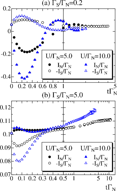
Figure 5: (Color online) Time evolution of the currents for the systems with $V/\Gamma_{N}=0.5$, $\Delta/\Gamma_{N}=0.5$, and $T=0$. Open (closed) symbols represent the current from the superconducting (normal) lead to the quantum dot when $\Gamma_{S}/\Gamma_{N}=0.2$ (a) and $\Gamma_{S}/\Gamma_{N}=5.0$ (b).

In the Kondo-singlet dominant region $(\Gamma_{S}/\Gamma_{N}=0.2)$, the interaction quench leads to a drastic change in the current $I_{N}$, in contrast to $I_{S}$, as shown in Fig. 5 (a). When $t\Gamma_{N}\sim 0.02$, the current $I_{N}$ changes its sign and a fairly large transient current flows against the bias voltage around $t\Gamma_{N}\sim 0.3$. This may be explained by the following. In the initial steady state, the particle number at the quantum dot is larger than the half filling. Therefore, the interaction quench tends to decrease the particle number at the quantum dot, which results in the decrease of both currents from the dots. In this case, there may be the relation $\Delta I_{S}/\Delta I_{N}\sim\Gamma_{N}/\Gamma_{S}$ around $t\sim 0$, which induces a large transient current between the quantum dot and the normal lead. As time progresses, the current $I_{N}$ turns over again and the system approaches the steady state. In the case $U/\Gamma_{N}=10.0$, the current largely fluctuates in the transient region $t\Gamma_{N}<1$ and the system may not reach the steady state around $t=t_{max}$. However, its oscillation rapidly relaxes and the steady current is expected to be around two currents at $t=t_{max}$.

On the other hand, when the superconducting lead tightly couples to the quantum dot ($\Gamma_{S}/\Gamma_{N}=5.0$), the currents are slightly changed by the interaction quench and the magnitudes of two currents approach each other around $t\Gamma_{N}\sim 0.5$, in contrast to the $\Gamma_{S}/\Gamma_{N}=0.2$ case. Nevertheless, we do not find the convergence in the current even around $t=t_{max}$, as shown in Fig. 5. This may originate from the time evolution of the Kondo resonance induced by the interaction quench. It is characterized by an exponentially small energy scale and should be slow to be built up in the case $\Gamma_{S}/\Gamma_{N}>1$. In this case, the steady current, as which the transient currents at $t=t_{max}$ are regarded in the paper, should be a lower bound of the correct value. Therefore, Monte Carlo simulations on longer contours are necessary to obtain the steady current more precisely.Werner

By performing similar calculations, we obtain the current-voltage characteristics of the systems with $\Gamma_{S}/\Gamma_{N}=0.2$ and $5.0$, as shown in Fig. 6. In the noninteracting case $(U=0)$, the system should be regarded as the normal-superconducting junction with a simple tunnel barrier. When $\Gamma_{S}/\Gamma_{N}$ is away from unity, the current rapidly increases around $V\sim\Delta$. This behavior is well described by the conventional BTK theory.BTK

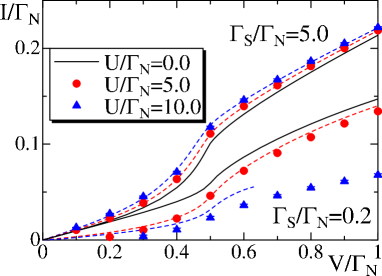
Figure 6: Current-voltage characteristics in the system with $\Gamma_{S}/\Gamma_{N}=0.2$ and $5.0$ when $\Delta/\Gamma_{N}=0.5$, $\epsilon_{d}+U/2=0$ and $T=0$. Circles and triangles represent the CTQMC results for $U/\Gamma_{N}=5.0$ and $10.0$ at $t=t_{max}$. Dashed lines represent the MPT results at the low temperature $T=0.01\Gamma_{N}$.Yamada

The introduction of the Coulomb interaction increases the current through the quantum dot tightly coupled to the superconducting lead $(\Gamma_{S}/\Gamma_{N}=5.0)$. In the case, we could not obtain the steady current precisely, as discussed above. Nevertheless, our results are consistent with those obtained by the MPT,Yamada which should be appropriate in this region. On the other hand, in the Kondo-singlet dominant region $(\Gamma_{S}/\Gamma_{N}=0.2)$, the Coulomb interaction decreases the current. In the MPT, the correlation effects are underestimated and the difference between two results becomes large in the strong coupling region.

We finally discuss the effect of electron correlations in the system with a fixed voltage $V/\Gamma_{N}=0.5$. The results for $U/\Gamma_{N}=0.0,5.0$, and $10.0$ are shown in Fig. 7.

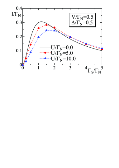
Figure 7: Currents functions of $\Gamma_{S}/\Gamma_{N}$ in the system with $V/\Gamma_{N}=0.5$, $\Delta/\Gamma_{N}=0.5$, $\epsilon_{d}+U/2=0$ and $T=0$.

The increase in $U$ monotonically decreases (increases) the current when $\Gamma_{S}/\Gamma_{N}<1.5(\Gamma_{S}/\Gamma_{N}>4)$. In the intermediate region $(\Gamma_{S}/\Gamma_{N}\sim 2.5)$, nonmonotonic behavior appears: the introduction of the interaction once increases the current in the proximity-induced on-dot pairing-dominant region. On the other hand, a further increase of the interaction decreases the current, where the Kondo singlet becomes dominant. The crossover behavior in the nonlinear response region may be similar to that in the linear response region of the quantum dot system with $\Delta\rightarrow\infty$,Tanaka where the zero bias conductance has a maximum around $\Gamma_{S}\sim U/2$. Therefore, we can say that the crossover between the Kondo-singlet and proximity-induced on-dot pairing dominant states affects the current-voltage characteristics under the high voltage beyond the superconducting gap $V\geq\Delta$.

In this paper, we have discussed the nonequilibrium phenomena of the quantum dot coupled to the normal and superconducting leads by means of the CTQMC method in the Keldysh formalism. It is an interesting problem how the local Coulomb interaction affects the Josephson current and multiple Andreev reflections in the quantum dot coupled to two superconducting leads, which is now under consideration.

V Summary

We have quantitatively studied the nonequilibrium phenomena through the quantum dot coupled to the normal and superconducting leads, extending the weak-coupling CTQMC method to treat the superconducting state in the Nambu formalism. We have confirmed that the obtained results are in good agreement with those obtained by the MPT in the weak coupling region and $\Gamma_{S}/\Gamma_{N}>1$.Yamada In the strong coupling region, we have clarified that the crossover between the Kondo singlet dominant and Cooper pairing singlet dominant regions affects the current-voltage characteristics. Transient currents induced by the interaction quench have been discussed.

VI Acknowledgments

We would like to thank R. Sakano, Y. Yamada, and P. Werner for valuable discussions. We also thank Y. Yamada for providing data, which we used in Figs. 4 and 6. This work was partly supported by the Global COE Program “Nanoscience and Quantum Physics” from the Ministry of Education, Culture, Sports, Science and Technology (MEXT) of Japan. A part of computations was carried out on TSUBAME2.0 at Global Scientific Information and Computing Center of Tokyo Institute of Technology and on the Supercomputer Center at the Institute for Solid State Physics, University of Tokyo. The simulations have been performed using some of the ALPS libraries. alps1.3

VII Appendix

VII.1 Calculation of noninteracting Green’s functions

Here, we explicitly show the impurity Green’s functions in the noninteracting case $U=0$. The Green’s functions for the impurity (quantum dot) site are represented in terms of the hybridization functions ${\hat{\Delta}}(\omega)$ as,

$${\hat{G}}_{0}^{R,A}(\omega) = \left[(\omega\pm i\eta){\hat{\sigma}}_{0}-\epsilon_{d}{\hat{\sigma}}_{z}-{\hat{\Delta}}^{R,A}(\omega)\right]^{-1}$$ (27)

$${\hat{G}}_{0}^{</>}(\omega) = {\hat{G}}_{0}^{R}(\omega){\hat{\Delta}}^{</>}(\omega){\hat{G}}_{0}^{A}(\omega),$$ (28)

where the hybridization functions are given as

$${\hat{\Delta}}^{R,A}(\omega) = \sum_{\alpha=N,S}{\hat{\Delta}}^{R,A}_{\alpha}(\omega)$$ (29)

$${\hat{\Delta}}^{R}_{N}(\omega) = -i\Gamma_{N}{\hat{\sigma}}_{0}$$ (30)

$${\hat{\Delta}}^{R}_{S}(\omega) = -i\Gamma_{S}\beta(\omega){\hat{M}}(\omega)$$ (31)

$${\hat{\Delta}}^{A}_{\alpha}(\omega) = \left[{\hat{\Delta}}^{R}_{\alpha}(\omega)\right]^{+}$$ (32)

$${\hat{\Delta}}^{<}_{N}(\omega) = 2i\Gamma_{N}{\hat{F}}(\omega)$$ (33)

$${\hat{\Delta}}^{<}_{S}(\omega) = 2i\Gamma_{S}{\rm Re}\left[\beta(\omega)\right]f(\omega){\hat{M}}(\omega)$$ (34)

$${\hat{\Delta}}^{>}_{N}(\omega) = -2i\Gamma_{N}\left({\hat{\sigma}}_{0}-{\hat{F}}(\omega)\right)$$ (35)

$${\hat{\Delta}}^{>}_{S}(\omega) = -2i\Gamma_{S}{\rm Re}\left[\beta(\omega)\right]\left[1-f(\omega)\right]{\hat{M}}(\omega),$$ (36)

where ${\hat{F}}(\omega)={\rm diag}\left[f(\omega-\mu_{N}),f(\omega+\mu_{N})\right],{\hat{M}}(\omega)={\hat{\sigma}}_{0}-\frac{\Delta_{S}}{\omega}{\hat{\sigma}}_{x}$ and $\beta(\omega)=\frac{|\omega|}{\sqrt{\omega^{2}-\Delta^{2}}}\theta(|\omega|-\Delta)-\frac{i\omega}{\sqrt{\Delta^{2}-\omega^{2}}}\theta(\Delta-|\omega|)$. Using the Fourier transformations, we obtain the lesser and greater Green’s functions eq. (13),

$${\hat{G}}_{0}^{</>}(t) = \int\frac{d\omega}{2\pi}{\hat{G}}_{0}^{</>}(\omega)e^{-i\omega t}.$$ (37)

VII.2 Calculation of ${\hat{A}}_{0\alpha}(t,t^{\prime})$

We obtain the expression of the matrix ${\hat{A}}_{0\alpha}(t,t^{\prime})$, which is necessary to calculate the current from the quantum dot to the $\alpha$th lead. We use the expression in previous papersWernerOka ; Jauho as

$$\left(\begin{array}[]{cc}{\hat{A}}_{0\alpha}^{R}&{\hat{A}}_{0\alpha}^{K}\\ 0&{\hat{A}}_{0\alpha}^{A}\end{array}\right)=-i\left(\begin{array}[]{cc}{\hat{G}}_{dd}^{R}&{\hat{G}}_{dd}^{K}\\ 0&{\hat{G}}_{dd}^{A}\end{array}\right)\left(\begin{array}[]{cc}{\hat{\Delta}}_{\alpha}^{R}&{\hat{\Delta}}_{\alpha}^{K}\\ 0&{\hat{\Delta}}_{\alpha}^{A}\end{array}\right),$$ (38)

where ${\hat{G}}_{dd}^{\eta}(\eta=R,A,K)$ is the retarded, advanced, and Keldysh impurity Green’s function for the Anderson model eq. (1) and ${\hat{\Delta}}^{K}_{\alpha}={\hat{\Delta}}^{<}_{\alpha}+{\hat{\Delta}}^{>}_{\alpha}$. Using the Fourier transformations as

$${\hat{A}}_{0\alpha}^{</>}(t) = \int\frac{d\omega}{2\pi}{\hat{A}}_{0\alpha}^{</>}(\omega)e^{-i\omega t},$$ (39)

$${\hat{A}}_{0\alpha}^{</>}(\omega) = \frac{1}{2}\left[{\hat{A}}_{0\alpha}^{K}(\omega)\mp{\hat{A}}_{0\alpha}^{R}(\omega)\pm{\hat{A}}_{0\alpha}^{A}(\omega)\right],$$ (40)

we obtain the matrix ${\hat{A}}_{0\alpha}(t,t^{\prime})$ in eq. (23).

References

- (1) L. P. Kouwenhoven, D. G. Austing, and S. Tarucha, Rep. Prog. Phys. 64, 701 (2001).
- (2) A. Eichler, M. Weiss, S. Oberholzer, C. Schonenberger, A. Levy Yeyati, J. C. Cuevas, and A. Martin-Rodero, Phys. Rev. Lett. 99, 126602 (2007).
- (3) M. R. Gräber, T. Nussbaumer, W. Belzig, and C. Schönenberger, Nanotechnology 15, S479 (2004).
- (4) L. Hofstetter, S. Csonka, J. Nygard, and C. Schönenberger, Nature 461, 960 (2009).
- (5) L. G. Herrmann, F. Portier, P. Roche, A. L. Yeyati, T. Kontos, and C. Strunk, Phys. Rev. Lett. 104, 026801 (2010).
- (6) R. S. Deacon, Y. Tanaka, A. Oiwa, R. Sakano, K. Yoshida, K. Shibata, K. Hirakawa, and S. Tarucha, Phys. Rev. Lett. 104, 076805 (2010).
- (7) R. S. Deacon, Y. Tanaka, A. Oiwa, R. Sakano, K. Yoshida, K. Shibata, K. Hirakawa, and S. Tarucha, Phys. Rev. B 81, 121308 (2010).
- (8) R. Fazio and R. Raimondi, Phys. Rev. Lett. 80, 2913 (1998).
- (9) P. Schwab and R. Raimondi, Phys. Rev. B 59, 1637 (1999).
- (10) A. A. Clerk, V. Ambegaokar, and S. Hershfield, Phys. Rev. B 61, 3555 (2000).
- (11) J. C. Cuevas, A. Levy Yeyati, and A. Martin-Rodero, Phys. Rev. B 63, 094515 (2001).
- (12) T. Domański, A. Donabidowicz, and K. I. Wysokiński, Phys. Rev. B 76, 104514 (2007).
- (13) Y. Tanaka, N. Kawakami, and A. Oguri, J. Phys. Soc. Jpn. 76, 074701 (2007).
- (14) V. Koerting, B. M. Andersen, K. Flensberg, and J. Paaske, Phys. Rev. B 82, 245108 (2010).
- (15) Y. Yamada, Y. Tanaka, and N. Kawakami, Phys. Rev. B 84, 075484 (2011).
- (16) J. Barański and T. Domański, Phys. Rev. B 84, 195424 (2011).
- (17) E. Gull, A. J. Millis, A. I. Lichtenstein, A. N. Rubtsov, M. Troyer, and P. Werner, Rev. Mod. Phys. 83, 349 (2011).
- (18) P. Werner, T. Oka, and A. J. Millis, Phys. Rev. B 79, 035320 (2009).
- (19) P. Werner, T. Oka, M. Eckstein, and A. J. Millis, Phys. Rev. B 81, 035108 (2010).
- (20) E. Gull, P. Werner, O. Parcollet, and M. Troyer, Europhys. Lett. 82 57003 (2008).
- (21) K. Satori, H. Shiba, O. Sakai, and Y. Shimizu, J. Phys. Soc. Jpn. 61, 3239 (1992).
- (22) A. Koga and P. Werner, J. Phys. Soc. Jpn. 79, 064401 (2010).
- (23) G. E. Blonder, M. Tinkham, and T. M. Klapwijk, Phys. Rev. B 25, 4515 (1982).
- (24) A. F. Albuquerque et al., J. Magn. Magn. Mater. 310, 1187 (2007).
- (25) A.-P. Jauho, N. S. Wingreen, and Y. Meir, Phys. Rev. B 50, 5528 (1994).