AGILE Mini-Calorimeter gamma-ray burst catalog

The Mini-Calorimeter of the AGILE satellite can observe the high-energy part of gamma-ray bursts with good timing capability. We present the data of the 85 hard gamma-ray bursts observed by the Mini-Calorimeter since the launch (April 2007) until October 2009. We report the timing data for 84 and spectral data for 21 bursts. The data table are available from the Strasbourg Astronomical Data Center (CDS) and the detailed data from the ASI Science Data Center (ASDC) .

1 Introduction

In recent years many instruments have been devoted to the study of the gamma-ray bursts (GRBs), which remain one of the most puzzling phenomena in the Universe.

The energy released from these events spans a wide spectral region, from radio to GeV, with great variations in temporal and spectral behavior (Mezaros (2006)). In most cases, the emission peaks in the range 50–500 keV; for this reason most of the instruments dedicated to GRBs are optimized for detection in this energy range.

The Mini-Calorimeter (MCAL) (Labanti et al. (2009)) onboard the AGILE satellite (Tavani et al. (2009)) is an instrument able to detect gamma-rays from $\sim$350 keV to 100 MeV region with a time resolution better than 2 ${\mu}$s. The main task of MCAL is to support the AGILE silicon tracker (Prest et al. (2003) , Bulgarelli et al. (2010)) in measuring the gamma-ray energy, but it is also used as an independent transients monitor and to investigate the high-energy part of GRBs (Marisaldi et al. (2008)).

Onboard the AGILE satellite the SuperAGILE (SA) instrument (Feroci et al. (2007)) also acts as a GRB monitor. It is a coded mask telescope operating in the energy range 15–45 keV with an angular resolution of 6 arcmin. Because of the very different energy ranges and the larger MCAL field of view (FOV) only a small fraction of the GRBs are detected by both instruments. The GRB data collected by SA are not homogeneous with the MCAL sample and are not considered in this paper.

Here we present a homogeneous sample of GRB data collected by MCAL between February 2008 and October 2009. During this period AGILE was operating in pointing mode, therefore a unique incoming direction in the reference frame of the spacecraft can be associated to each GRB. Since October 2009, AGILE is operating in spinning mode, due to a reaction-wheel failure, scanning a large fraction of the sky with a typical angular velocity of a few degrees per second. The GRB data collected in spinning mode need different analysis methods and will be the subject of a forthcoming study.

In Section 2 we briefly describe the MCAL instrument, in Section 3 we describe the data collection and processing, Section 4 deals with the temporal analysis of the GRBs, Section 5 deals with the spectral analysis, and Section 6 presents our conclusions.

2 Instrument

The Mini-Calorimeter of the AGILE Satellite has been fully described elsewhere (Labanti et al. (2009)): it consists of an array of 30 CsI(Tl) bars, each one of size $15\times 23\times 375\,\mathrm{mm}^{3}$, arranged in two layers with the bars aligned along orthogonal directions for a total thickness of 3 cm.

The scintillation light produced by the interacting gamma-rays is collected at each end of the bars by photo-diodes (PD); the attenuation of the light transmitted along the bar can be represented by an exponential decay; the decay coefficient has an average value of $0.028\,\mathrm{cm}^{-1}$ and has been measured for each bar before the final assembly of the instrument. The energy released in the bar and the event position along the bar are obtained according to the exponential decay law, as described in a previous paper (Labanti et al. (2009)). Measurements have shown that this is a reasonable approximation and fails only for energy released at the very end of the bars, where geometrical effects dominate over attenuation.

A discriminator circuit with programmable threshold receives the sum of the electric signals from the PDs; when the sum is higher than the threshold, the PDs signals are sent to an ADC, time-tagged and stored in a circular buffer. Because of the light attenuation, this electric signal threshold does not correspond to a fixed energy threshold: the bars are more sensitive to low-energy events near the photo-diodes than at the center of the bars. The PDs are characterized by their gain ($\mathrm{e}^{-}/\mathrm{keV}$) and the zero-level signal (offset). These parameters have been measured for each PD before launch and are used to evaluate the photon energy (Labanti et al. (2009)).

The MCAL instrument is situated below the silicon tracker, but its FOV is not limited to the FOV of the tracker and acts as an all-sky monitor. The effective area of the detector is between 200 and 500 $\mathrm{cm}^{2}$, depending on photon energy and angle (Labanti et al. (2009)).

A complex, fully programmable trigger logic for transient event detection is implemented on-board (Fuschino et al. (2008)). This trigger logic is based on the counts given by a number of detector rate-meters (DR): four independent rate-meters are obtained by dividing each MCAL layer into two parts and summing the signals from the bars of each part. The DR counts are integrated over three energy ranges ($<1.4\mathrm{MeV},1.4-3.0\mathrm{MeV},>3.0\mathrm{MeV}$) and six time windows (1, 16, 64, 256, 1024 and 8192 ms). These integrated counts are compared to the integrated background signal with a background integration-time chosen among seven time intervals (8, 16, 32, 65, 131, 262 and 524 s) and delayed with respect to the DR integration times. For the 1-ms and 16-ms time windows, the MCAL is considered as a whole and not divided into four parts. An additional moving time window of $300\,\mu$s duration is implemented for the detection of very short transients.

A partial trigger signal is issued for each DR if the counts exceed a given threshold. The trigger logic compares all partial triggers; a GRB trigger signal is issued only if a proper combination of partial triggers is obtained, otherwise the event is rejected. Different combinations of DRs, thresholds, time windows, and background integration-times, can be chosen; moreover the trigger criterion can be either static or dynamic: in the static criterion the threshold is fixed, while in the dynamic criterion the threshold is proportional to the standard deviation of the background. The GRB end time is determined by the time at which all DRs decrease below given thresholds; static and dynamic criteria are also implemented for the GRB ending time choice (TSTOP time). The trigger logic has been tuned during the first months of the mission, to optimize sensitivity and telemetry load, and minimizing the rate of false-positive triggers. The configuration implemented onboard requires that at least two partial triggers on different DR are issued at the same time for time windows larger than 16 ms. For these time windows the dynamic criterion was set, requiring that a partial trigger is issued only when the count rate exceeds the measured background rate by at least five standard deviations. The requirement for two simultaneous partial triggers implies a rather uniform involvement of all detection planes and helps to reject local enhancements generated by, for example, noise increase. For time windows of 16 ms and shorter, the static trigger criterion was set, requiring at least seven, ten and ten counts in the $300\;\mu s$, 1 ms and 16 ms time windows, respectively.

When a GRB trigger is issued, data are transmitted to the ground station on a photon-by-photon basis. Together with the GRB data, many seconds of data before and after the GRB are sent to ensure a proper estimate of the background level.

Since the end of the commissioning phase, MCAL and SuperAGILE, are part of the third InterPlanetary Network (IPN) (Hurley et al. (2004)), devoted to the localizing of GRBs by means of triangulation among different spacecrafts.

3 Data processing and selection

AGILE is on a nearly equatorial low-Earth orbit with a period of about 90 minutes; the MCAL data are sent once per orbit by the spacecraft to the ASI ground station based in Malindi, Kenya, during the ground-station contact phase. The data are processed as soon as they are received. The relevant data processing steps are energy evaluation, data selection and photon list production.

• Gamma-ray energy release evaluation: The energy released in each bar is evaluated; most of the events deposit energy in a single bar. For multiple events, i.e., those involving more than one bar, we attribute to the event the sum of the energies released in all different bars.

• On-ground data selection: the data stream transmitted to the ground station for each GRB trigger is visually inspected, and spurious triggers due to known electronic noise issues are discarded. Data in which only very short timescale triggers (trigger on the 16-ms time window or less) are activated are also carefully inspected but, since they are mostly relevant for terrestrial gamma-ray flashes (TGF) science (Marisaldi et al. (2010)), they are not included in the present work.

• Photon list production: for each accepted trigger a photon list is produced. The photon list contains the time of each detected photon, and the energy released in each bar. Many seconds of background data before and after the GRB data are included, as specified in the trigger logic configuration.

This catalog includes 76 GRBs triggered on the 64-ms timescale and longer, plus nine GRBs triggered on the 16-ms timescale. For the 64-ms sample 81% of the GRBs activate the lower energy triggers $(E<1.4MeV)$ and only 17% and 2% the upper energy ones; the triggers for the four time windows of 64, 256, 1024 and 8192 ms represent 12, 34, 29, and 25% of the total. Triggers on timescales up to 16 ms where included only if the events were confirmed by at least another spacecraft belonging to the IPN. This latter criterion results in nine triggers on the 16 ms timescale only.

The GRBs included in the catalog are listed in Table LABEL:maindata. The column contact is the number of the AGILE orbit in which the GRB was detected. The trigger time is the time of the GRB trigger signal (seconds from 1 January 2004); the celestial coordinates RA and DEC are given in decimal degrees and obtained from the relevant GCN circulars , the absence of decimals means that approximate values are obtained from the IPN data available online (Hurley et al. (2013)). The column TH is the angle between the AGILE pointing direction and the direction of the GRB. The column other detections reports if the data for the GRB have been published also by other missions, or a GCN circular is issued for the detection. The GRBs for which very high energy gamma-rays have been detected by the AGILE Tracker (TR) have been highlighted.

The MCAL is an all-sky instrument, but for geometrical reasons it is more sensitive to GRBs coming from the AGILE pointing direction. In the years 2008-2009 AGILE was used to follow gamma transients pointing for many months on sources on the Galactic Plane and on Galactic Center. In Fig. 1 the GRB sky distribution is shown in galactic coordinates; a greater number of GRBs can be seen on the Galactic Center zone and around the Galactic Plane. A list of AGILE pointings for most of the reference period is reported by Pittori (Pittori et al. (2009)).

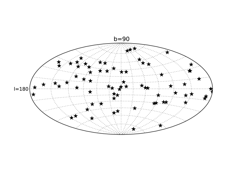
Figure 1: Sky distribution of MCAL GRBs in galactic coordinates. The Galactic Center is at the center of the figure.

4 Temporal analysis

For the temporal analysis of the GRBs we computed the $T_{90}$ and $T_{50}$ time intervals, defined as the intervals containing the 90% and 50% of the total counts of gamma rays above the background. Our $T_{50}$ and $T_{90}$ measure the time width of the high energy part of the GRB (above $\sim 300\,keV$) which is seen by MCAL. We adopted the method of Koshut (Koshut et al. (1996)):

• the counts in the photon list are grouped in temporal bins of 0.01 s; from which we obtained a light curve for the GRB.

• By visual analysis of the light curve, two background-only time intervals were identified, one before and one after the burst. We kept these time intervals as long as possible, to achieve a better background subtraction; for their visual identification, a binning of 0.1 sec was sometimes used, which does not allow for an analysis of short GRBs, but gives less noisy time profiles.

• The two selected intervals were used to define a background model in the GRB time interval by a low-order interpolating polynomial (most of the time first order was sufficient).

• The cumulative integral of the background-subtracted counts was computed for each time bin; thus we obtained a cumulative time profile.

• The mean values of the two background-only intervals in the cumulative time profile were computed. These values define a minimum and a maximum fluence level, expressed in counts. The mean value of the background region before the GRB should theoretically be zero, but in practice, as also noticed by Koshut (Koshut et al. (1996)), it can be different from zero, due to background fluctuations.

• A GRB fluence (in counts) is defined as the difference between the maximum and the minimum fluence level. The time interval between the points in which the cumulative time profile is 5% and 95% of the GRB fluence defines the $T_{90}$ interval. In the same way, the time points at 25% and 75% define $T_{50}$. The uncertainties in $T_{50}$ and $T_{90}$ were computed following Koshut (Koshut et al. (1996)).

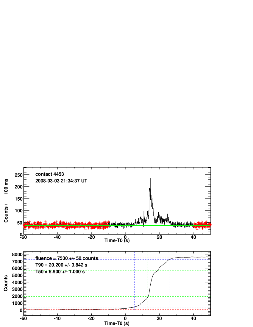
Figure 2: GRB 080303B, time analysis. In the upper plot we show the GRB time profile; the two background zones are the time intervals: -60/-10 and 40/50 s. In the lower plot we show the cumulative time profile; the lines defining the fluence, $T_{50}$ and $T_{90}$ are shown as well. For a better visualization, a 0.1 s time binning has been used in this figure.

In Fig. 2 an example of the procedure is shown; in the upper panel we plot the time profile of GRB 080803B along with the background zones and the line fitting the background values; in the lower panel the cumulative integral is shown along with the lines defining the fluence minimum and maximum levels, the $T_{90}$ and $T_{50}$ intervals.

We performed a time analysis for 84 GRBs from our sample; GRB 080603B (contact number 5750) is confirmed by the IPN network, but too faint for a time analysis. The results are shown in Table LABEL:T5090. $T_{50}$ and $T_{90}$, their starting times and the boundaries of the background intervals are reported. All times are given in seconds measured from the trigger time. The column $T_{90}$ fluence contains the background-subtracted counts in the GRB region. Our $T_{50}$ and $T_{90}$ measurements refer to the high-energy part of the GRB; for this reason the duration measured by other instruments, which are sensitive to lower energies, are often longer (see Paciesas et al. (2012)): we did not see the lower energy tails of some GRBs.

The main features of our sample are summarized in Table 3; our average value for $T_{90}$ is about 13 sec. We had no very long GRBs in our sample.

	$T_{90}$ (s)	$T_{50}$ (s)	Counts in $T_{90}$
min. value	0.04	0.02	66
max. value	89.81	21.44	12472
average	12.61	4.64	1822

Table 3: GRB temporal analysis summary

The distributions of $T_{90}$ and $T_{50}$ are shown in Fig. 3 and Fig. 4. The data are consistent with the well-known bimodal distribution (Kouveliotou et al. (1993)). We see a clear peak for long GRBs and a peak for short GRBs that is less resolved due to the limited statistics for this group. The two maxima are observed at $T_{90}\sim 0.3$ s and $T_{90}\sim 8$ s. Considering as short the GRB with $T_{90}<2$ s, we have 21% of short GRB, a value consistent with the results of instruments operating in the hard X-ray range: Paciesas reported a value of 18% for the Fermi data (with an uncertainty of 3-4%) and of 24% for the BATSE catalog (Paciesas et al. (2012)); see also Kouveliotou (Kouveliotou et al. (1993)) and Frontera (Frontera et al. (2009)) for previous samples.

Figure 3: $T_{90}$ distribution.

Figure 4: $T_{50}$ distribution.

5 Spectral analysis

Only a subsample of the GRBs in the catalog have enough photons to allow for a spectral analysis. Background subtraction is a critical point in the analysis, and we can obtain reliable spectra only for GRBs with more than $\sim 1000$ background-subtracted counts in the $T_{90}$ interval. The MCAL effective area has a cutoff below $\sim 350$ keV, for this reason a fit of our data with a Band function (Band et al. (1993)) is, in most cases, not suitable, since we cannot constrain the low-energy part of the spectra. We instead used a simple power law function to describe the GRB high-energy part between 400 keV and 5 MeV: $f(E)=N\times(E/E0)^{-\beta}$, with a photon index $\beta$ that is similar to the $\beta$ index in the GRB Band model. We processed here all GRBs in the same way, fitting with the same simple power-law function, to obtain a set of homogeneous results. A detailed analysis for some high flux GRBs, such as GRB 090510, has been published elsewhere (Giuliani et al. (2008), Giuliani et al. (2010)).

The uncertainty in the response matrix for gamma-rays coming from below the instrument is higher. These gamma-rays cross the service module of the satellite before hitting MCAL. For this reason we considered only the GRBs with a direction of less than 90 degrees from the AGILE pointing direction.

Our procedure consisted of the following steps:

• Obtaining the spectra of the detected GRB photons from the photon list. The photon list produced by the MCAL onboard software was used to obtain the spectrum of energy released in MCAL by the GRB during the $T_{90}$ time interval. A background spectrum was also extracted from the data, summing over a time interval as long as possible before the trigger (30–50 s). A large background interval smoothes the short-time oscillations in the background, which can introduce errors when the burst fluence is low. The energies released in all bars that correspond to a single event, were summed; the bars with an energy lower than 400 keV were discarded in this phase to minimize the contribution of possible uncertainties in diode calibrations, which mostly affect the low-energy events. The spectra were binned at a fixed bin size of 50 keV, up to 10 MeV (200 bins). The spectra were produced in the FITS format (Wells et al, (1981)).

• Dead-time correction. The anti-coincidence (AC) veto system of the AGILE tracker (Perotti et al. (2006)) is active during the GRB. This system also affects the MCAL counts, blocking MCAL for $5.4\,\mu$s for each AC event. With a particle background rate of $\sim 10$ kHz and a GRB photon rate of $\sim 15-30$ kHz, this dead-time effect amounts to about $10-20\%$. To account for this effect, we considered an average of the AC rates during the GRB and the background interval and decreased the exposure time in a consistent way.

• Fitting. The XSPEC program (Arnaud (1996)) was used for fitting. We used the XSPEC CSTAT statistic, a modified version of the Cash statistic (Cash, (1979)), which is more appropriate when counts are low. A response matrix and auxiliary response files were computed for each GRB with the same energy binning of the spectra and considering the angle between the GRB direction and the AGILE axis. The discarding of bars with a low energy deposit was accounted for. The method used for the computation of the response matrix will be detailed in a forthcoming article (2013, in preparation ).

  A power law function $f(E)=N\times(E/500\,keV)^{-\beta}$ was used for the fits over the energy range 400–5000 keV.

In Fig. 5, an example of a GRB background-subtracted spectrum is shown along with the folded model from the XSPEC fit (continuous line); the error bars are one-sigma poisson errors. Some energy bins over $\sim 1.5$ MeV were merged.

Figure 5: GRB 080916C: spectral data and folded model from XSPEC (continuous line). The power law model is $\sim E^{-2.24}$.

Spectral data are shown in Table LABEL:spectra, where the spectral index $\beta$ and the normalization parameter $N$ are reported along with the model flux integrated over the energy interval $400-5000$ keV and averaged over $T_{90}$. We also report the fluence, integrated over $T_{90}$, the $CSTAT$ value, and the number of degrees of freedom (dof) from the XSPEC fit.

In Fig. 6 we show the distribution of the power law index $\beta$. Most of the values are between 2 and 3. A similar distribution is found for the Band model $\beta$ parameter in the Fermi sample of Bissaldi (Bissaldi et al. (2011)) or in the Fermi spectral catalog (Goldstein et al. (2012)), but we see a somewhat greater number of high $\beta$ GRBs. We are still investigating this effect; a detailed comparison of our spectral data with other samples will be presented in a forthcoming paper (2013, in preparation ). The model fluence distribution is shown in Fig. 7.

Figure 6: Power law index $\beta$ distribution.

Figure 7: Fluence distribution.

6 Conclusions

We presented the GRB data collected with the AGILE MCAL instrument between February 2008 and October 2009. The effective area of MCAL decreases below $\sim 350$ keV, and this GRB sample consists of hard events, with data up to the MeV range. Our temporal analysis shows a $T_{90}$ distribution consistent with other studies, in spite of our higher energy range. We also presented a spectral analysis for a subsample of our data: we fitted our data with a simple power law. Our spectral index is comparable to the $\beta$ parameter in the classical Band GRB model. Our results are similar to other studies, but with somewhat lower spectral indexes.

Table 5: Main GRB data. Boldface GRBs have high-energy photons detected by the AGILE Tracker. For the detection by other missions the following acronyms are used: INT for the INTEGRAL satellite (Winkler et al. (2003)), RH for RHESSI (Lin et al. (2002)), SW for the SWIFT satellite (Gehrels et al. (2004)), KW for KONUS/Wind (Aptekar et al. (1995)), SU for Suzaku (Mitsuda et al. (2007)), FE for Fermi (Michelson et al. (2010), Meegan (2009)), SA for SuperAGILE, TR for the AGILE Tracker, OPT means optical or radio followup, IPN means that a tentative GRB position was obtained by IPN data or that a GCN was issued by the IPN.

Contact	Trigger time	Name	Date	RA	DEC	TH	Other detections
ID	sec.from 01-01-2004		UTC	deg.	deg.	deg.
4172	129942289.420	080212B	2008-02-12 23:04:49.420	123	22	98	IPN
4453	131664877.825	080303B	2008-03-03 21:34:37.825	270	-26	108	IPN
4673	133014356.656	080319C	2008-03-19 12:25:56.656	259.0	55.4	84	INT KW SU SW OPT
4798	133776179.856	080328	2008-03-28 08:02:59.856	80.5	47.5	155	INT KW SU SW OPT
4946	134685725.108	080407	2008-04-07 20:42:05.108	183	20	76	KW IPN
5030	135199576.492	080413	2008-04-13 19:26:16.492	287.3	-27.7	49	KW SW OPT
5370	137281445.197	080507B	2008-05-07 21:44:05.197	247	-24	95	IPN
5462	137843756.822	080514B	2008-05-14 09:55:56.822	322.8	0.7	37	KW SU IPN/SA TR SW OPT
5665	139084070.650	080528	2008-05-28 18:27:50.650	77	28	93	KW IPN
5692	139248696.743	080530	2008-05-30 16:11:36.743	186	0	69	IPN
5750	139606694.696	080603B	2008-06-03 19:38:14.696	176.5	68.1	74	INT KW SW OPT
5799	139903643.150	080607	2008-06-07 06:07:23.150	194.9	15.9	114	INT KW RH SW OPT
5837	140136578.898	080609	2008-06-09 22:49:38.898	262	-26	132	IPN
5852	140231946.977	080611	2008-06-11 01:19:06.977	83	27	85	IPN
5887	140440358.003	080613B	2008-06-13 11:12:38.003	173.8	-7.1	39	INT KW SW OPT
6044	141402060.830	080624	2008-06-24 14:21:00.830	…	…	…
6258	142712152.973	080709	2008-07-09 18:15:52.973	245	-22	91	IPN
6328	143142769.240	080714	2008-07-14 17:52:49.240	188.1	-60.3	13	KW SW OPT
6345	143246921.106	080715	2008-07-15 22:48:41.106	214.7	65.9	66	IPN FE
6422	143720706.723	080721	2008-07-21 10:25:06.723	224.5	-11.7	49	KW RH INT SW
6452	143904198.133	080723B	2008-07-23 13:23:18.133	176.8	-60.2	13	INT KW SA SW OPT
6458	143941060.261	080723D	2008-07-23 23:37:40.261	105.3	71.1	134	FE
6506	144231210.935	080727B	2008-07-27 08:13:30.935	276.9	1.2	101	KW SW OPT
6600	144807750.714	080803B	2008-08-03 00:22:30.714	108	22	50	IPN
6800	146029932.250	080817	2008-08-17 03:52:12.250	151.3	-19.3	57	FE
6919	146758428.560	080825C	2008-08-25 14:13:48.560	232.2	-4.9	75	FE
7073	147700735.012	080905	2008-09-05 11:58:55.012	287.67	-18.87	139	FR SW OPT
7083	147762311.241	080906B	2008-09-06 05:05:11.241	182.8	-6.4	115	FE
7221	148608766.336	080916C	2008-09-16 00:12:46.336	119.8	-56.6	86	FE IPN KW SW OPT
7255	148815876.398	080918	2008-09-18 09:44:36.398	22	14	107	IPN
7445	149980665.476	081001	2008-10-01 21:17:45.476	276.6	-8.7	21	KW SA SW OPT
7483	150211576.844	081004	2008-10-04 13:26:16.844	113	-3	147	IPN
7889	152700294.277	081102B	2008-11-02 08:44:54.277	231.2	35.2	53	FE
7935	152976706.752	081105	2008-11-05 13:31:46.752	4.0	3.5	66	IPN SW
8006	153411942.992	081110	2008-11-10 14:25:42.992	123.6	21.2	124	FE
8165	154384526.221	081121	2008-11-21 20:35:26.221	89.3	-60.6	141	FE KW SW OPT
8216	154698820.603	081125	2008-11-25 11:53:40.603	42.7	-18.9	84	FE
8330	155397093.361	081203B	2008-12-03 13:51:33.361	228.8	44.4	69	KW SU SW OPT
8420	155950316.320	081209	2008-12-09 23:31:56.320	45.3	63.5	52	FE IPN KW
8502	156451717.870	081215	2008-12-15 18:48:37.870	135.0	53.8	89	FE IPN KW
8593	157006438.184	081222	2008-12-22 04:53:58.184	22.75	-34.10	88	FE KW SW OPT
8631	157238275.145	081224	2008-12-24 21:17:55.145	201.7	75.1	59	FE SU SW
8712	157735152.060	081230B	2008-12-30 15:19:12.060	…	…	…
8747	157949728.040	090102	2009-01-02 02:55:28.040	128.2	33.1	94	KW SW
9156	160452584.144	090131	2009-01-31 02:09:44.144	353.0	16.4	55	FE SU
9179	160595218.112	090201	2009-02-01 17:46:58.112	92.0	-46.6	139	KW SW OPT
9260	161088448.472	090207B	2009-02-07 10:47:28.472	…	…	…
9508	162605543.649	090225	2009-02-25 00:12:23.649	358.1	61.0	19	FE
9553	162881600.901	090228	2009-02-28 04:53:20.901	106.8	-24.3	111	FE
9621	163300476.010	090305B	2009-03-05 01:14:36.010	155.1	68.1	120	FE
9731	163969232.676	090312	2009-03-12 19:00:32.676	…	…	…
9951	165317810.892	090328	2009-03-28 09:36:50.892	90.9	-41.9	105	FE KW SW
9955	165344824.903	090328B	2009-03-28 17:07:04.903	155.7	33.4	132	FE IPN
9972	165446602.621	090329	2009-03-29 21:23:22.621	…	…	…
10007	165659724.000	090401B	2009-04-01 08:35:24.000	95.09	-8.96	41	KW SA SU TR SW OPT
10139	166467473.377	090410	2009-04-10 16:57:53.377	334.96	15.41	54	SU SW OPT
10335	167667129.448	090424	2009-04-24 14:12:09.448	189.5	16.8	103	FE SU SW OPT
10364	167848413.139	090426C	2009-04-26 16:33:33.202	82.7	-9.7	143	FE
10383	167959586.511	090427	2009-04-27 23:26:26.511	235.9	13.5	71	IPN KW
10553	168999780.445	090510	2009-05-10 00:23:00.445	333.56	-26.61	61	FE SU SW TR OPT
10741	170155676.304	090523	2009-05-23 09:27:56.304	30	11	108	IPN
10814	170598152.774	090528B	2009-05-28 12:22:32.774	312.2	32.7	28	FE SU
10832	170707316.602	090529C	2009-05-29 18:41:56.602	…	…	…
10860	170879756.431	090531B	2009-05-31 18:35:56.492	252.07	-36.02	82	FE SW OPT
10999	171732798.963	090610	2009-06-10 15:33:25.936	84.2	35.4	84	FE
11027	171903051.103	090612	2009-06-12 14:50:51.103	81.1	17.8	92	FE
11092	172299598.562	090617	2009-06-17 04:59:58.562	78.9	15.7	91	FE SU
11108	172398504.772	090618	2009-06-18 08:28:24.772	294.0	78.4	38	FE KW SA SU SW OPT
11137	172575386.596	090620	2009-06-20 09:36:26.596	237.4	61.2	57	FE
11404	174209913.464	090709	2009-07-09 07:38:33.464	289.9	60.7	48	KW SA SU SW OPT
11513	174876569.696	090717	2009-07-17 00:49:29.696	86.8	-64.2	152	FE SU
11514	174883231.619	090717B	2009-07-17 02:40:31.619	247.0	23.0	68	FE
11541	175051886.412	090719	2009-07-19 01:31:26.412	341.3	-67.9	133	FE KW
11565	175194176.902	090720B	2009-07-20 17:02:56.905	203.0	-54.8	155	FE KW IPN
11851	176945288.503	090809B	2009-08-09 23:28:08.503	93.5	0.1	89	FE
11914	177324581.259	090814C	2009-08-14 08:49:41.259	332.5	58.9	154	FE
11993	177813526.664	090820	2009-08-20 00:38:46.664	87.7	27.0	130	FE OPT
12044	178128673.156	090823	2009-08-23 16:11:13.156	128.67	60.6	141	IPN KW SW
12107	178511020.971	090828	2009-08-28 02:23:40.971	124.4	-26.1	72	FE
12129	178646894.468	090829	2009-08-29 16:08:14.468	329.2	-34.2	64	FE SU
12156	178811964.864	090831D	2009-08-31 13:59:24.864	…	…	…
12269	179505087.102	090908	2009-09-08 14:31:27.102	…	…	…
12466	180709001.651	090922	2009-09-22 12:56:42.137	17.1	74.3	117	FE
12616	181629345.746	091003	2009-10-03 04:35:45.746	251.1	37.2	67	FE KW SU SW OPT
12714	182227390.920	091010	2009-10-10 02:43:10.920	298.7	-22.5	9	FE KW SA SU SW OPT

Table 5: continued. Main GRB data.

Table 6: GRB temporal data.

Contact	Name	$T_{90}$	$T_{90}$ start	$T_{50}$	$T_{50}$ start	$T_{90}$ Fluence	Background intervals
ID		sec.	sec. from trigger	sec.	sec. from trigger	counts	sec. from trigger
4172	080212B	6.16 $\pm$ 3.83	0.265	2.11 $\pm$ 0.46	1.125	1931 $\pm$ 154	-60	-10	20	30
4453	080303B	20.09 $\pm$ 3.45	5.345	5.84 $\pm$ 0.96	13.165	6775 $\pm$ 215	-30	-10	40	50
4673	080319C	19.22 $\pm$ 3.64	-10.815	4.41 $\pm$ 3.36	0.295	1101 $\pm$ 142	-30	-15	15	30
4798	080328	15.42 $\pm$ 11.14	4.355	11.83 $\pm$ 2.53	6.425	1079 $\pm$ 102	-30	-5	25	40
4946	080407	20.16 $\pm$ 1.86	2.215	8.72 $\pm$ 0.74	6.905	7427 $\pm$ 159	-30	-15	30	50
5030	080413	30.28 $\pm$ 15.59	-8.395	7.13 $\pm$ 2.47	7.175	873 $\pm$ 144	-30	-10	25	30
5370	080507B	0.22 $\pm$ 0.25	0.045	0.03 $\pm$ 0.04	0.225	83 $\pm$ 18	-0.5	0	1	2
5462	080514B	6.09 $\pm$ 4.74	0.245	3.73 $\pm$ 0.96	2.075	1347 $\pm$ 117	-20	-5	10	20
5665	080528	0.24 $\pm$ 1.71	0.025	0.11 $\pm$ 0.06	0.065	296 $\pm$ 48	-10	-1	1	7
5692	080530	1.43 $\pm$ 2.19	-0.365	0.16 $\pm$ 0.14	0.215	457 $\pm$ 51	-5	-1	1	5
5799	080607	10.38 $\pm$ 3.03	1.175	4.75 $\pm$ 0.49	4.585	4165 $\pm$ 119	-80	-10	20	30
5837	080609	20.60 $\pm$ 0.61	1.105	10.42 $\pm$ 0.92	6.115	12472 $\pm$ 180	-80	-10	30	45
5852	080611	0.04 $\pm$ 0.06	0.035	0.02 $\pm$ 0.01	0.055	342 $\pm$ 24	-50	-1	1	20
5887	080613B	18.33 $\pm$ 6.71	-0.045	9.24 $\pm$ 2.65	1.645	1465 $\pm$ 147	-20	-5	20	40
6044	080624	23.64 $\pm$ 8.28	-14.565	12.52 $\pm$ 3.18	-10.165	1005 $\pm$ 149	-40	-20	20	30
6258	080709	20.94 $\pm$ 1.84	1.825	11.74 $\pm$ 0.50	4.225	7944 $\pm$ 163	-40	-10	30	50
6328	080714	39.65 $\pm$ 20.64	-7.085	11.99 $\pm$ 8.12	3.565	1021 $\pm$ 158	-18	-10	35	50
6345	080715	26.39 $\pm$ 7.72	-6.065	7.06 $\pm$ 17.82	-0.505	464 $\pm$ 137	-25	-10	20	40
6422	080721	15.64 $\pm$ 1.13	1.045	5.97 $\pm$ 0.51	9.355	5460 $\pm$ 198	-25	-10	20	40
6452	080723B	45.65 $\pm$ 1.09	-43.975	13.44 $\pm$ 1.03	-14.365	3443 $\pm$ 206	-70	-50	10	40
6458	080723D	43.56 $\pm$ 2.70	4.115	8.40 $\pm$ 5.83	12.445	3930 $\pm$ 235	-70	-10	60	70
6506	080727B	1.99 $\pm$ 1.18	-0.135	0.45 $\pm$ 1.12	0.095	227 $\pm$ 54	-5	-1	5	10
6600	080803B	17.50 $\pm$ 13.55	0.285	5.47 $\pm$ 4.47	3.895	617 $\pm$ 144	-40	-5	20	30
6800	080817	17.84 $\pm$ 2.03	-0.625	9.44 $\pm$ 0.77	3.795	4239 $\pm$ 175	-30	-10	30	60
6919	080825C	3.67 $\pm$ 1.29	0.605	1.51 $\pm$ 0.25	1.425	1069 $\pm$ 69	-10	-1	7	15
7073	080905	1.26 $\pm$ 3.53	0.005	0.80 $\pm$ 0.79	0.135	164 $\pm$ 42	-10	-1	2	6
7083	080906B	4.78 $\pm$ 6.87	0.555	0.95 $\pm$ 3.50	0.865	317 $\pm$ 94	-20	-3	10	20
7221	080916C	39.31 $\pm$ 7.35	0.695	21.44 $\pm$ 5.16	3.985	3778 $\pm$ 215	-60	-10	50	80
7255	080918	4.64 $\pm$ 2.87	-0.915	0.85 $\pm$ 0.15	1.285	1395 $\pm$ 89	-8	-3	5	10
7445	081001	5.40 $\pm$ 3.10	-1.495	1.24 $\pm$ 1.75	0.165	500 $\pm$ 68	-6	-2	7	10
7483	081004	0.13 $\pm$ 1.73	0.005	0.04 $\pm$ 0.05	0.015	197 $\pm$ 45	-5	-1	1	5
7889	081102B	7.30 $\pm$ 14.06	3.525	1.70 $\pm$ 2.08	5.945	346 $\pm$ 74	-30	0	15	50
7935	081105	6.17 $\pm$ 1.63	0.045	2.50 $\pm$ 0.68	1.265	3154 $\pm$ 107	-30	-2	8	40
8006	081110	3.64 $\pm$ 1.76	-2.000	0.64 $\pm$ 0.38	0.135	489 $\pm$ 44	-30	-2	25	40
8165	081121	18.96 $\pm$ 2.61	0.935	6.38 $\pm$ 2.40	7.915	1805 $\pm$ 123	-25	-1	25	40
8216	081125	4.12 $\pm$ 5.34	-2.225	1.94 $\pm$ 1.27	-1.135	360 $\pm$ 60	-25	-3	5	25
8330	081203B	20.16 $\pm$ 14.88	0.955	5.28 $\pm$ 2.60	6.885	1027 $\pm$ 116	-40	-4	20	40
8420	081209	0.13 $\pm$ 0.29	0.045	0.06 $\pm$ 0.04	0.055	184 $\pm$ 30	-0.5	-0.2	0.4	0.8
8502	081215	4.92 $\pm$ 0.98	-0.585	2.46 $\pm$ 0.40	0.385	2365 $\pm$ 118	-20	-5	10	20
8593	081222	6.69 $\pm$ 6.71	0.995	3.48 $\pm$ 2.95	2.125	362 $\pm$ 85	-5	-1	10	15
8631	081224	7.80 $\pm$ 2.81	0.385	2.45 $\pm$ 0.46	1.135	2706 $\pm$ 133	-20	-5	15	30
8712	081230C	2.52 $\pm$ 1.81	0.045	1.19 $\pm$ 1.39	0.395	225 $\pm$ 60	-5	-1	5	10
8747	090102	14.19 $\pm$ 3.00	5.205	9.27 $\pm$ 1.43	8.455	1137 $\pm$ 106	-20	-5	25	40
9156	090131	32.41 $\pm$ 11.12	-16.790	9.74 $\pm$ 19.45	0.100	624 $\pm$ 154	-28	-20	15	40
9179	090201	25.47 $\pm$ 8.81	-12.045	10.83 $\pm$ 2.43	1.105	2200 $\pm$ 195	-40	-20	20	40
9260	090207B	0.10 $\pm$ 0.07	-0.005	0.06 $\pm$ 0.04	0.005	66 $\pm$ 13	-1	-0.2	0.2	0.3
9508	090225	0.28 $\pm$ 0.16	-0.005	0.09 $\pm$ 0.13	0.095	82 $\pm$ 15	-0.5	0	0.4	0.8
9553	090228	0.09 $\pm$ 0.53	0.005	0.06 $\pm$ 0.02	0.015	316 $\pm$ 29	-0.8	-0.2	0.4	0.8
9621	090305B	0.53 $\pm$ 0.97	-0.145	0.27 $\pm$ 0.13	0.025	186 $\pm$ 33	-10	-2	1	5
9731	090312	8.49 $\pm$ 14.91	2.545	4.45 $\pm$ 2.04	5.325	636 $\pm$ 77	-22	-5	15	35
9951	090328	26.98 $\pm$ 4.59	0.275	10.72 $\pm$ 1.78	6.605	4420 $\pm$ 175	-25	-5	35	50
9955	090328B	0.15 $\pm$ 0.22	-0.025	0.07 $\pm$ 0.04	0.005	167 $\pm$ 26	-0.6	-0.2	0.3	1
9972	090329	4.15 $\pm$ 4.13	-1.505	1.39 $\pm$ 0.40	0.205	834 $\pm$ 37	-18	-4	10	30
10007	090401B	8.98 $\pm$ 0.29	0.915	1.6 $\pm$ 0.19	7.355	4041 $\pm$ 119	-10	-1	12	22
10139	090410	12.19 $\pm$ 12.60	2.035	4.07 $\pm$ 4.61	5.065	592 $\pm$ 102	-5	0	20	30
10335	090424	6.78 $\pm$ 6.41	-2.755	2.96 $\pm$ 0.47	0.355	854 $\pm$ 92	-20	-5	5	15
10364	090426C	4.17 $\pm$ 4.60	-1.395	1.17 $\pm$ 1.56	0.425	216 $\pm$ 63	-8	-2	15	25
10383	090427	2.97 $\pm$ 1.03	8.045	0.98 $\pm$ 0.06	8.825	6325 $\pm$ 179	-20	-5	15	30
10553	090510	5.19 $\pm$ 5.91	0.065	0.29 $\pm$ 0.22	0.125	1553 $\pm$ 64	-20	-5	15	30
10741	090523	1.12 $\pm$ 1.05	-0.855	0.13 $\pm$ 0.12	0.055	188 $\pm$ 33	-25	-1	2	10
10814	090528B	30.36 $\pm$ 19.88	1.285	15.92 $\pm$ 9.16	7.205	1271 $\pm$ 151	-30	-5	35	50
10832	090529D	15.83 $\pm$ 8.09	-5.005	3.73 $\pm$ 11.31	4.355	386 $\pm$ 81	-30	-5	15	32
10860	090531B	1.66 $\pm$ 2.06	-0.975	0.43 $\pm$ 0.38	0.015	258 $\pm$ 54	-50	-2	10	40
10999	090610	8.82 $\pm$ 7.38	-1.415	8.82 $\pm$ 7.38	3.165	293 $\pm$ 77	-25	-2	20	45
11027	090612	3.12 $\pm$ 8.38	-0.845	1.32 $\pm$ 0.81	0.125	716 $\pm$ 109	-25	-5	5	25
11092	090617	0.67 $\pm$ 1.17	-0.305	0.20 $\pm$ 0.31	-0.005	83 $\pm$ 19	-4	-0.3	0.3	4
11108	090618	89.81 $\pm$ 11.74	3.055	9.54 $\pm$ 3.20	63.285	10614 $\pm$ 271	-30	-5	140	150
11137	090620	13.61 $\pm$ 3.76	-7.695	3.67 $\pm$ 2.55	-1.275	737 $\pm$ 101	-40	-10	15	25
11404	090709	53.22 $\pm$ 11.00	3.385	20.67 $\pm$ 2.88	23.465	4242 $\pm$ 225	-40	-10	70	90
11513	090717	8.42 $\pm$ 12.02	3.375	5.19 $\pm$ 3.68	4.875	460 $\pm$ 74	-15	-5	15	30
11514	090717B	0.37 $\pm$ 1.06	-0.035	0.11 $\pm$ 0.11	0.135	87 $\pm$ 20	-3	-1	1	2
11541	090719	7.28 $\pm$ 13.24	0.275	3.97 $\pm$ 1.03	1.715	2860 $\pm$ 181	-20	-15	20	40
11565	090720B	6.21 $\pm$ 0.14	0.015	5.73 $\pm$ 0.33	0.135	1234 $\pm$ 83	-30	-9	25	45
11851	090809B	6.81 $\pm$ 14.56	6.655	1.71 $\pm$ 1.04	8.055	877 $\pm$ 114	-10	-1	20	30
11914	090814C	0.28 $\pm$ 1.64	-0.075	0.11 $\pm$ 0.11	-0.005	137 $\pm$ 28	-10	-0.5	1	2
11993	090820	8.18 $\pm$ 2.03	1.055	3.36 $\pm$ 0.25	2.435	6454 $\pm$ 123	-30	-10	20	40
12044	090823	5.33 $\pm$ 8.37	-0.325	2.44 $\pm$ 1.26	0.925	806 $\pm$ 107	-20	-5	10	25
12107	090828	8.46 $\pm$ 9.72	-3.175	2.90 $\pm$ 1.72	0.125	537 $\pm$ 88	-20	-5	10	25
12129	090829	23.24 $\pm$ 5.19	1.595	7.04 $\pm$ 1.14	7.895	4244 $\pm$ 174	-30	-5	35	50
12156	090831D	2.10 $\pm$ 0.23	-2.005	0.73 $\pm$ 1.10	-0.695	169 $\pm$ 15	-6	-2	15	20
12269	090908C	4.05 $\pm$ 6.57	0.065	0.72 $\pm$ 0.68	0.305	380 $\pm$ 54	-10	-5	5	10
12466	090922	15.92 $\pm$ 5.24	-9.045	4.71 $\pm$ 10.00	-0.075	466 $\pm$ 87	-60	-10	20	30
12616	091003	24.68 $\pm$ 11.40	-4.125	16.45 $\pm$ 1.17	2.365	2397 $\pm$ 170	-40	-10	30	45
12714	091010	3.17 $\pm$ 1.95	-1.495	2.24 $\pm$ 1.93	-1.225	260 $\pm$ 67	-8	-3	4	8

Table 6: continued. GRB temporal data.

Table 7: GRB spectral data.

Contact	Name	$\beta$	$N$	Flux	Fluence	$CSTAT$	dof
ID			$ph./cm^{2}/s/keV$	$ergs/cm^{2}/s$	$ergs/cm^{2}$
			at 500 keV	400-5000 keV	in $T_{90}$
4673	080319C	2.26 $+$ 0.43 - 0.34	5.42E-04 $\pm$ 1.13E-04	4.25e-07	8.17e-06	85.28	89
4946	080407	2.72 $+$ 0.08 - 0.08	3.02E-03 $\pm$ 8.15E-05	1.65e-06	3.33e-05	116.66	89
5462	080514B	2.61 $+$ 0.25 - 0.21	1.64E-03 $\pm$ 5.14E-05	9.68e-07	5.90e-06	84.31	89
5887	080613B	2.19 $+$ 0.22 - 0.20	5.45E-04 $\pm$ 6.15E-05	4.57e-07	8.38e-06	113.42	89
6328	080714	2.14 $+$ 1.24 - 0.83	2.09E-04 $\pm$ 7.27E-05	1.83e-07	7.26e-06	59.23	89
6452	080723B	2.93 $+$ 0.34 - 0.29	6.26E-04 $\pm$ 9.22E-05	3.00e-07	1.37e-05	90.09	89
6800	080817	2.47 $+$ 0.11 - 0.11	1.52E-03 $\pm$ 6.64E-05	1.00e-06	1.78e-05	107.25	89
6919	080825C	2.39 $+$ 0.17 - 0.19	2.36E-03 $\pm$ 9.37E-05	1.65e-06	6.06e-06	69.03	89
7221	080916C	2.24 $+$ 0.15 - 0.14	1.33E-03 $\pm$ 1.32E-04	1.06e-06	4.17e-05	90.58	89
7935	081105	2.21 $+$ 0.09 - 0.09	2.94E-03 $\pm$ 1.80E-04	2.42e-06	1.49e-05	138.05	89
8330	081203B	2.65 $+$ 0.36 - 0.30	6.08E-04 $\pm$ 6.97E-05	3.50e-07	7.06e-06	100.44	89
8502	081215	2.43 $+$ 0.10 - 0.10	1.04E-02 $\pm$ 4.15E-04	7.07e-06	3.48e-05	86.40	89
8631	081224	2.79 $+$ 0.12 - 0.11	3.28E-03 $\pm$ 1.66E-04	1.71e-06	1.33e-05	97.05	89
10007	090401B	2.14 $+$ 0.07 - 0.07	2.79E-03 $\pm$ 1.48E-04	2.45e-06	2.20e-05	84.37	89
10383	090427	2.30 $+$ 0.05 - 0.05	1.55E-02 $\pm$ 3.48E-04	1.18e-05	3.50e-05	108.55	89
10553	090510	1.43 $+$ 0.11 - 0.11	1.08E-03 $\pm$ 7.28E-04	2.16e-06	1.12e-05	71.59	89
10814	090528B	2.55 $+$ 0.31 - 0.27	4.45E-04 $\pm$ 6.90E-05	2.75e-07	8.35e-06	75.48	89
11108	090618	2.73 $+$ 0.27 - 0.32	6.32E-04 $\pm$ 6.33E-05	3.43e-07	3.08e-05	78.96	89
11404	090709	2.66 $+$ 0.19 - 0.17	6.51E-04 $\pm$ 6.36E-05	3.71e-07	1.97e-05	96.29	89
12129	090829	2.38 $+$ 0.12 - 0.11	1.14E-03 $\pm$ 5.35E-05	8.07e-07	1.88e-05	130.16	89
12616	091003	2.72 $+$ 0.26 - 0.23	7.57E-04 $\pm$ 7.11E-05	4.13e-07	1.02e-05	109.16	89
Detailed analysis published (Giuliani et al. (2008)).
Detailed analysis published (Moretti et al. (2009), Giuliani et al. (2009)).
Detailed analysis published (Giuliani et al. (2010)).

Table 7: continued. GRB spectral data.