Abstract

We consider a generalization of the holographic Schwinger effect proposed by Semenoff and Zarembo to the case with constant electric and magnetic fields. There are two ways to turn on magnetic fields, i) the probe D3-brane picture and ii) the string world-sheet picture. In the former picture, magnetic fields both perpendicular and parallel to the electric field are activated by a Lorentz transformation and a spatial rotation. In the latter one, the classical solutions of the string world-sheet corresponding to circular Wilson loops are generalized to contain two additional parameters encoding the presence of magnetic fields.

1 Introduction

In the vacuum of quantum electrodynamics (QED), virtual $e^{-}$ and $e^{+}$ pairs are incessantly created and annihilated. The pairs can become real particles in the presence of strong electric-field. This realization is well known as a novel non-perturbative phenomenon called the Schwinger effect [1, 2]. The production rate $\Gamma$ of the pairs in a homogeneous electric field is computed in the weak-coupling and weak-field approximation like

$$\Gamma=\frac{(eE)^{2}}{(2\pi)^{3}}{\rm e}^{-\frac{\pi m^{2}}{eE}}\,.$$

It has not been observed in nature yet, but it is expected to be done in the near future [3, 4] (For a recent review on the Schwinger effect, see [5]).

The derivation of the pair-production rate was refined to an arbitrary coupling [6]. This generalization leads to examining the expectation value of a circular Wilson loop in the computational process. It can be evaluated using the weak-field condition for an arbitrary coupling and eventually gives a small correction. The result is given by [6]

$$\Gamma=\frac{(eE)^{2}}{(2\pi)^{3}}{\rm e}^{-\frac{\pi m^{2}}{eE}+\frac{1}{4}e^{2}}\,.$$ (1.1)

The similar formula holds for magnetic monopoles [7]. Then it is fair to ask what happens when the computation of (1.1) is applied to the AdS/CFT correspondence [8, 9, 10].

Some observables in strongly-coupled gauge-theories are computed in terms of the classical gravitational-theory via the AdS/CFT correspondence [8, 9, 10]. An example is the expectation value of a Wilson loop, which can be evaluated as the minimal surface of the string world-sheet attaching the boundary [11, 12]. Hence this is an advantage in the holographic setup. On the other hand, $U(1)$ gauge theories like QED cannot be argued directly because $SU(N)$ ones simply correspond to gravitational theories. Thus one has to consider an intricate setup to discuss the Schwinger effect in the holographic scenario.

The setup we are concerned with is the correspondence between type IIB string theory on $\text{AdS}_{5}\times S^{5}$ and ${\cal N}=4$ super Yang-Mills (SYM) theory in four dimensions. One way to realize a $U(1)$ gauge theory in this setup is to spontaneously break the gauge group from $SU(N+1)$ to $SU(N)\times U(1)$ . Then the computation in the gauge-theory side is almost the same as in scalar QED in four dimensions. It is of paramount importance that the holographic description is available to evaluate the expectation value of a circular Wilson loop. The Schwinger effect in this direction is studied in [13, 14, 15, 16].

In this note we consider a generalization of the scenario by Semenoff and Zarembo [14] to the pair productions in the presence of electric and magnetic fields. There are two ways to turn on magnetic fields, i) the probe D3-brane picture and ii) the string world-sheet picture. In the former picture, magnetic fields both perpendicular and parallel to the electric field are activated by a Lorentz transformation and a spatial rotation. In the latter one, the classical solutions of the string world-sheet corresponding to circular Wilson loops are generalized to contain two additional parameters encoding the presence of magnetic fields.

This note is organized as follows. In section 2 we prepare the setup to consider the holographic Schwinger effect. In section 3 we consider a generalization of the holographic Schwinger effect to the case with electric and magnetic fields. We show two ways to turn on magnetic fields. Section 4 is devoted to conclusion and discussion.

2 Holographic Schwinger effect

Let us consider a stack of $N+1$ D3-branes on which the ${\mathcal{N}}=4$ $SU(N+1)$ SYM theory in four dimensions is realized as the low-energy effective theory. Then separating a single D3-brane leads to the Higgs mechanism in the theory.

The $SU(N+1)$ gauge field $\hat{A}_{\mu}~{}(\mu=0,\ldots,3)$ , the real scalar fields $\hat{\Phi}_{I}~{}(I=1,\ldots,6)$ and the fermion fields $\hat{\Psi}$ are decomposed as follows:

$$\hat{A}_{\mu}=\begin{pmatrix}A_{\mu}&\omega_{\mu}\\ \omega_{\mu}^{\dagger}&a_{\mu}\end{pmatrix}\,,\quad\hat{\Phi}_{I}=\begin{pmatrix}\Phi_{I}&\omega_{I}\\ \omega_{I}^{\dagger}&m\theta_{I}+\phi_{I}\end{pmatrix}\,,\quad\hat{\Psi}=\begin{pmatrix}\Psi&\chi\\ \chi^{\dagger}&\psi\end{pmatrix}\,.$$ (2.1)

Here the diagonal components $A_{\mu}~{}[a_{\mu}]$, $\Phi_{I}~{}[\phi_{I}]$, and $\Psi~{}[\psi]$ are the $SU(N)~{}[U(1)]$ gauge, the scalar and the fermion fields, respectively. The non-diagonal components $\omega_{\mu}$, $\omega_{I}$, and $\chi$ transform as the fundamental representation of $SU(N)$ and form the W-boson multiplet. Finally $m\theta_{I}$ are the vacuum expectation values, where $\theta_{I}$ satisfy $\sum_{I}(\theta_{I})^{2}=1$ . Then $\phi_{I}$ are regarded as fluctuations around them.

According to the decomposition (2.1), the original action $S_{{\cal N}=4}^{SU(N+1)}$ is decomposed into the three parts,

$$S_{{\cal N}=4}^{SU(N+1)}\quad\longrightarrow\quad S_{{\cal N}=4}^{SU(N)}+S_{{\cal N}=4}^{U(1)}+S_{{\rm W}}\,,$$

and each of them is described below,

$$1)\mbox{~{}~{}${\mathcal{N}}=4$ $SU(N)$ SYM theory, $S_{{\cal N}=4}^{SU(N)}$}\,,\qquad 2)\mbox{~{}~{}${\mathcal{N}}=4$ $U(1)$ SYM theory, $S_{{\cal N}=4}^{U(1)}$}\,,$$

$$3)\mbox{~{}~{}the action of the W-boson multiplet, $S_{\rm W}$}\,.$$

For later purpose, we shall write down the concrete expression of $S_{\rm W}$ only,

$$S_{\text{W}}=\frac{1}{g_{\text{YM}}^{2}}\int\!{\rm d}^{4}x\,\left[(D_{\mu}\omega_{I})^{\dagger}D^{\mu}\omega_{I}+\omega_{I}^{\dagger}(\Phi_{K}-m\theta_{K})^{2}\omega_{I}-m^{2}\omega_{I}^{\dagger}\theta_{I}\theta_{J}\omega_{J}+\cdots\right]\,.$$ (2.2)

The covariant derivative is defined as

$$D_{\mu}\equiv\partial_{\mu}-iA_{\mu}+ia_{\mu}\,,$$ (2.3)

and the ellipsis represents the kinematic terms of the other components of the W-boson multiplet and the other interaction terms.

After taking the near-horizon limit, a stack of $N$ D3-branes is replaced by the $\text{AdS}_{5}\times S^{5}$ geometry,

$${\rm d}s^{2}=\frac{r^{2}}{L^{2}}\eta_{\mu\nu}{\rm d}x^{\mu}{\rm d}x^{\nu}+\frac{L^{2}}{r^{2}}{\rm d}r^{2}+L^{2}{\rm d}\Omega_{(5)}^{2}\,,$$ (2.4)

where ${\rm d}\Omega_{(5)}^{2}$ is the metric of the five-dimensional sphere with unit radius and $L$ is the common radius of AdS₅ and $S^{5}$ . The metric $\eta_{\mu\nu}$ describes the Minkowski spacetime. The isolated D3-brane is described as a probe D3-brane extending in AdS₅ .

In the scenario of the holographic Schwinger effect by Semenoff and Zarembo [14], the $U(1)$ gauge field is treated as a constant external field, while the $SU(N)$ gauge field is regarded as a dynamical field. Then, following the work of Affleck, Alvarez and Manton [6], the production rate can be evaluated. The resulting expression includes the expectation value of a circular Wilson loop of $SU(N)$ gauge field. It is a point that one has to evaluate the non-abelian Wilson loop rather than the abelian one in comparison to the QED case. Thus it is not an easy task any more in the field-theory framework, but now the holographic computation based on the string world-sheet is applicable.

2.1 Properties of an electric field from D3-brane action

Let us first anticipate the expected behavior of an electric field from the point of view of the Dirac-Born-Infeld (DBI) action describing the probe D3-brane.

The square-root part of the probe D3-brane action is given by

$$S_{\text{DBI}}=-T_{\text{D3}}\int\!{\rm d}^{4}x\,\sqrt{-\det(g_{\mu\nu}+{\cal F}_{\mu\nu})}\,,$$

where the D3-brane tension $T_{\rm D3}$ and the world-volume flux ${\cal F}_{\mu\nu}$ are, respectively,

$$T_{\text{D3}}=\frac{1}{g_{\text{s}}(2\pi)^{3}\alpha^{\prime 2}}\,,\qquad{\cal F}_{\mu\nu}\equiv B_{\mu\nu}+2\pi\alpha^{\prime}F_{\mu\nu}\,.$$

The string tension is given by $T_{\rm F}=1/2\pi\alpha^{\prime}$ and the string coupling constant is $g_{\text{s}}$ . Then $B_{\mu\nu}$ is the pull-back of the NS-NS two-form $B_{\it 2}$ and $F_{\mu\nu}$ is the world-volume flux living on the D3-brane.

Henceforth we will consider the case that the probe D3-brane is located at $r=r_{0}$ in the AdS space rather than near the boundary, as depicted in Fig. 1. In addition, an electric field $E$ $(={\cal F}_{01}/2\pi\alpha^{\prime})$ is equipped with the probe D3-brane. Then the DBI action can be rewritten as

$$S_{\text{DBI}}=-T_{\text{D3}}\frac{r_{0}^{4}}{L^{4}}\int\!{\rm d}^{4}x\,\sqrt{1-\frac{(2\pi\alpha^{\prime})^{2}L^{4}}{r_{0}^{4}}E^{2}}\,.$$ (2.5)

When the electric field is given by

$$E_{\text{DBI}}=\frac{1}{2\pi\alpha^{\prime}}\frac{r_{0}^{2}}{L^{2}}\,,$$ (2.6)

the DBI action vanishes. When the electric field grows more than (2.6), the DBI action becomes ill-defined.

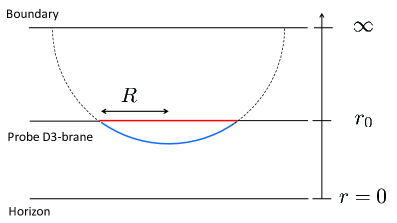
Figure 1: The location of the probe D3-brane and the configuration of the string world-sheet.

Let us write (2.6) with the gauge-theory parameters. $r_{0}$ is related with the mass of the W-boson multiplet, $m$. The mass is the energy of a single string stretching between the probe D3-brane at $r=r_{0}$ and the horizon at $r=0$ . The induced metric for the string is $g_{ab}={\text{diag}}(-r^{2}/L^{2},L^{2}/r^{2})$ and hence the mass is given by

$$m=T_{\text{F}}\int_{0}^{r_{0}}\!{\rm d}r\,\sqrt{-\det g_{ab}}\,=\frac{r_{0}}{2\pi\alpha^{\prime}}\,.$$ (2.7)

Using (2.7) and eliminating $r_{0}$ , the electric field (2.6) is rewritten as

$$E_{\text{DBI}}=\frac{2\pi m^{2}}{\sqrt{\lambda}}\,.$$ (2.8)

2.2 Pair creation in ${\cal N}=4$ SYM

It is a turn to focus upon a pair creation of $\omega_{I}$ , for simplicity, in the Higgsed ${\cal N}=4$ $SU(N+1)$ SYM theory in the large $N$ limit. We will work in the Euclidean siganture below, unless otherwise stated.

First of all, let us point out the difference from the QED case [2, 6]. In the $\mathcal{N}=4$ SYM theory, the number of $\omega_{I}$ is increased and hence the production rate is proportional to $N$ . Then the loop corrections of the W-boson multiplet and a $U(1)$ photon are suppressed in the large $N$ limit because the ones are proportional to $1/N$ and $g_{\text{YM}}^{2}=\lambda/N$ , respectively. The $SU(N)$ gauge field is regarded as a fluctuation and the $U(1)$ gauge field is done as an external field. That is, the covariant derivative is given by

$$D_{\mu}=\partial_{\mu}-iA_{\mu}+ia_{\mu}^{\text{ex}}\,.$$ (2.9)

The pair-production rate (per unit volume) $\Gamma$ is generally written as

$$\Gamma=2\,\text{Im}\,\varepsilon_{0}\,,$$

in terms of the vacuum energy density $\varepsilon_{0}$ . In the ${\cal N}=4$ SYM theory, it is represented by

$$V_{4}\Gamma =-2\,\text{Im}\,\ln\int\!{\cal D}A{\cal D}\Phi{\cal D}\omega\,{\rm e}^{-S_{{\cal N}=4}^{SU(N)}-S_{\text{W}}}$$

$$=-2\,\text{Im}\,\ln\int\!{\cal D}A{\cal D}\Phi\,{\rm e}^{-S_{{\cal N}=4}^{SU(N)}-S_{\text{eff}}}\,,$$ (2.10)

where the effective action is given by

$$S_{\text{eff}} =-\ln\int\!{\cal D}\omega\,{\rm e}^{-S_{\text{W}}}$$

$$=\frac{5N}{2}\text{tr}_{\text{op}}\,\text{tr}_{SU(N)}\,\ln\left[-D_{\mu}D^{\mu}+(\Phi_{K}-m\theta_{K})^{2}\right]\,.$$ (2.11)

In the last expression, $\text{tr}_{\text{op}}$ is the trace about eigenvalues of operators and $\text{tr}_{SU(N)}$ is the trace about $SU(N)$. The factor $5N/2$ comes from the number of $\omega_{I}$ .

Then the production rate is evaluated as

$$V_{4}\Gamma =-2\,\text{Im}\,\ln\int{\cal D}A{\cal D}\Phi\,{\rm e}^{-S_{{\cal N}=4}^{SU(N)}-S_{\text{eff}}}\simeq 2\,\text{Im}\,\langle S_{\text{eff}}\rangle$$

$$=5N\,\text{Im}\,\left\langle\text{tr}_{\text{op}}\,\text{tr}_{SU(N)}\,\ln\left[-D_{\mu}D^{\mu}+\left(\Phi_{K}-m\theta_{K}\right)^{2}\right]\right\rangle\,,$$ (2.12)

where the expectation value has been utilized,

$$\left\langle g[A,\Phi]\right\rangle=\frac{\displaystyle\int\!{\cal D}A{\cal D}\Phi\,g[A,\Phi]\,{\rm e}^{-S_{{\cal N}=4}^{SU(N)}[A,\Phi]}}{\displaystyle\int\!{\cal D}A{\cal D}\Phi\,{\rm e}^{-S_{{\cal N}=4}^{SU(N)}[A,\Phi]}}\,.$$

By using the Schwinger parametrization and the quantum-mechanical path-integral, the production rate is expressed as

$$V_{4}\Gamma =-5N\,\text{Im}\,\int_{0}^{\infty}\frac{{\rm d}T}{T}\left\langle\text{tr}_{SU(N)}{\cal P}\exp\left(-\frac{1}{2}D_{\mu}D^{\mu}T+\frac{1}{2}(\Phi_{K}-m\theta_{K})^{2}T\right)\right\rangle$$

$$=-5N\,\text{Im}\,\int_{0}^{\infty}\frac{{\rm d}T}{T}\int\!{\cal D}x\,\left\langle\text{tr}_{SU(N)}{\cal P}{\rm e}^{-S_{\rm inst}}\right\rangle\,,$$

$$S_{\rm inst}\equiv\int_{0}^{T}{\rm d}\tau\,\left[\frac{1}{2}\dot{x}^{2}-iA_{\mu}\dot{x}^{\mu}+ia_{\mu}^{\text{ex}}\dot{x}^{\mu}+\frac{1}{2}\left(\Phi_{K}-m\theta_{K}\right)^{2}\right]\,.$$ (2.13)

The above expression contains the path ordering $\cal P$ because the $SU(N)$ gauge field is concerned in the present case.

Then let us evaluate the $T$-integral. The argument below is the same as the derivation in Appendix A of [19], up to minor modifications. The integral to be evaluated is

$$\int_{0}^{\infty}\frac{{\rm d}T}{T}\,{\rm e}^{-S_{\rm inst}}\,.$$ (2.14)

The first and fourth terms in (2.13) are not invariant under the reparametrization of $\tau$ .

Consider the transformation $\tau\rightarrow\tilde{\tau}(\tau)$ such that $\tilde{\tau}(0)=0,\tilde{\tau}(T)=T$ are satisfied. By defining $c(\tau)\equiv{\rm d}\tilde{\tau}/{\rm d}\tau$ , the $T$-integral (2.14) is rewritten as the path integral about $c(\tau)$,

$$\int\!{\cal D}c\,\frac{1}{c}\,\exp\left(-\int_{0}^{1}{\rm d}\tau\left[\frac{1}{2c}\dot{x}^{2}+\frac{c}{2}\left(\Phi_{K}-m\theta_{K}\right)^{2}\right]\right)\,,$$ (2.15)

where we have ignored the terms invariant under the reparametrization of $\tau$ . The stationary point about $c(\tau)$ is estimated as

$$c(\tau)\simeq\frac{\sqrt{\dot{x}^{2}(\tau)}}{m}\,,$$ (2.16)

by assuming that $m$ is very large.

By the saddle-point approximation about $c(\tau)$, we obtain

$$V_{4}\Gamma =-5N\,\text{Im}\,\int\!{\cal D}x\,g[x(\tau)]\,{\rm e}^{-S_{\rm particle}[x]}\left\langle W[x]\right\rangle\,,$$ (2.17)

$$S_{\rm particle}[x]\equiv m\sqrt{\int_{0}^{1}{\rm d}\tau\,\dot{x}^{2}}-i\int_{0}^{1}{\rm d}\tau\,a_{\mu}^{\text{ex}}\dot{x}^{\mu}\,,$$ (2.18)

$$W[x]=\text{tr}_{SU(N)}{\cal P}\exp\left(\int\!{\rm d}\tau\left[iA_{\mu}(x)\dot{x}^{\mu}+\Phi_{I}\theta_{I}\sqrt{\dot{x}^{2}}\right]\right)\,,$$ (2.19)

where $g[x(\tau)]$ is a functional. $g[x(\tau)]$ does not influence the classical solution about the steepest descent about $x(\tau)$. Then the exponential factor in $\Gamma$ is not changed by $g[x(\tau)]$ and $W[x]$ is the $SU(N)$ Wilson loop.

Now let us consider how to evaluate (2.17). In the QED case [6], the exponential part is evaluated with the steepest descent by using the instanton solution, and then the expectation value of the Wilson loop is exactly computed because the gauge field is $U(1)$ . In the present case the exponential factor can be evaluated in the same way. The Wilson loop is now non-abelian but it is possible to apply the holographic computation. Naively, one may expect that this computation works well.

The classical solutions are obtained by solving the equations of motion obtained from $S_{\rm particle}$ . Then they describe the circular motion with the radius $m/E$ . By putting them into (2.19), its shape is fixed to be circular. Since the expectation value of the circular Wilson loop is evaluated as [19, 20]

$$\langle W[x]\rangle={\rm e}^{n\sqrt{\lambda}}\qquad(\mbox{wrapped $n$ times})$$

in the holographic computation, the resulting classical action is given by

$$S_{\text{cl}}^{(n)}=\left(\frac{\pi m^{2}}{E}-\sqrt{\lambda}\right)n\,.$$ (2.20)

Then the production rate is evaluated as

$$\Gamma\sim{\rm e}^{-S_{\text{cl}}^{(1)}}=\exp\left(-\frac{\pi m^{2}}{E}+\sqrt{\lambda}\right)\,.$$ (2.21)

From this expression, one can read off the critical flux as

$$E=\frac{\pi m^{2}}{\sqrt{\lambda}}\,,$$ (2.22)

so that the production rate is not exponentially suppressed no longer. However, the critical value (2.22) is different from the critical value (2.8) estimated from the DBI argument.

In the above calculation of the circular Wilson loop, the probe D3-brane is located at $r=\infty$ in the radial direction. This conflicts with the assumption to place the probe D3-brane at $r=r_{0}$ rather than $r=\infty$ . Hereupon Semenoff and Zarembo [14] proposed that the exponential factor and the expectation value of the Wilson loop should be replaced by the Nambu-Goto (NG) action of a single string attaching on the probe D3-brane at $r=r_{0}$ and the coupling to $B_{\it 2}$ . That is, the production rate is expected to be

$$\Gamma\sim{\rm e}^{-S_{\text{st}}}\,,\qquad S_{\text{st}}=S_{\text{NG}}+S_{B_{\it 2}}\,,$$

$$S_{\text{NG}}\equiv T_{\text{F}}\int\!{\rm d}^{2}\sigma\,\sqrt{\det G_{ab}}\,,\qquad S_{B_{\it 2}}\equiv-T_{\text{F}}\int\!{\rm d}^{2}\sigma\,B_{\mu\nu}\partial_{\tau}x^{\mu}\partial_{\sigma}x^{\nu}\,,$$

where $G_{ab}$ is the induced metric on the string world-sheet with the coordinates $\sigma^{a}=(\tau,\sigma)$ . This proposal is supported by the coincidence of the critical flux.

Let us evaluate the production rate by following the Semenoff and Zarembo’s proposal. We first find the minimal surface of the string with a circular boundary on the probe D3-brane at $r=r_{0}$ . When the radius of the Wilson loop is $R$ on the probe D3-brane, the solutions of the string world-sheet are given by [20]

$$x_{0} =x(\sigma)\cos(2n\pi\tau)\,,\qquad x_{1}=x(\sigma)\sin(2n\pi\tau)\,,$$

$$r =r(\sigma)\,,\qquad x^{2}+\left(\frac{L^{2}}{r}\right)^{2}=R^{2}+\left(\frac{L^{2}}{r_{0}}\right)^{2}\,.$$ (2.23)

A possible representation of the solutions is

$$x(\sigma)=\frac{1}{\cosh\left(2n\pi\sigma\right)}\sqrt{R^{2}+\left(\frac{L^{2}}{r_{0}}\right)^{2}}\,,\quad r(\sigma)=\frac{L^{2}}{\tanh\left(2n\pi\sigma\right){\sqrt{R^{2}+(L^{2}/r_{0})^{2}}}}\,.$$ (2.24)

By putting the solutions (2.23) into the string action, we obtain

$$S_{\text{NG}}=2n\pi T_{\text{F}}L^{2}\left[\sqrt{\left(\frac{Rr_{0}}{L^{2}}\right)^{2}+1}-1\right]\,,\qquad S_{B_{\it 2}}=-n\pi ER^{2}\,,$$ (2.25)

where we have defined as

$$E\equiv T_{\text{F}}B_{01}\,,$$

and $E$ is interpreted as an electric field in the gauge-theory side.

The string boundary condition on the probe D3-brane is the mixed (Robin) due to the presence of $B_{\it 2}$ like

$${\cal P}_{\mu}+T_{\text{F}}B_{\mu\nu}\partial_{\tau}x^{\nu}\Big{|}_{r(\tau,\sigma_{0})=r_{0}}=0\,,\quad{\cal P}_{\mu}\equiv\frac{\delta S_{\text{NG}}}{\delta\left(\partial_{\sigma}x^{\mu}\right)}=T_{\text{F}}\sqrt{\det G}G^{\sigma\sigma}g_{\mu\nu}\partial_{\sigma}x^{\nu}\,.$$

The value of $R$ is determined from this boundary condition,

$$R=\frac{L^{2}}{r_{0}}\sqrt{\frac{{\cal E}^{2}}{E^{2}}-1}\,,\qquad{\cal E}=T_{\text{F}}\frac{r_{0}^{2}}{L^{2}}\,.$$ (2.26)

Note that the value of $R$ is also determined by taking a variation of the classical action with respect to $R$ in [14, 16]. The two ways lead to the identical result.

Then ${\cal E}$ is regarded as the critical value of the electric field so that $R\geq 0$ . This is the same as the critical value (2.8) obtained from the argument on the DBI action. In terms of the gauge-theory parameters, the production rate is given by

$$\Gamma\sim\exp\left(-\frac{\sqrt{\lambda}}{2}\left[\sqrt{\frac{{\cal E}}{E}}-\sqrt{\frac{E}{{\cal E}}}\;\right]^{2}\right)\,,\qquad{\cal E}=\frac{2\pi m^{2}}{\sqrt{\lambda}}\,.$$ (2.27)

The exponential suppression disappears when $E={\cal E}$ . The production rate is approximated to

$$\Gamma\sim\exp\left(-\frac{\pi m^{2}}{E}+\sqrt{\lambda}\right)\,,$$ (2.28)

when $E\ll{\cal E}$ . This agrees with (2.21).

3 Turning on magnetic fields

Let us discuss a generalization of the scenario proposed in [14] by including magnetic fields both perpendicular and parallel to an electric field.

3.1 From the DBI action of the probe D3-brane

We first consider the case that magnetic fields $B_{\parallel}$ and $B_{\perp}$ on $x$-direction and $y$-direction, respectively, as well as an electric field $E$ on $x$-direction. Then the square root in the DBI action of the probe D3-brane is expressed in the Lorentzian signature like

$$-\det\begin{pmatrix}-r_{0}^{2}/L^{2}&-2\pi\alpha^{\prime}E&&\\ 2\pi\alpha^{\prime}E&r_{0}^{2}/L^{2}&&2\pi\alpha^{\prime}B_{\perp}\\ &&r_{0}^{2}/L^{2}&-2\pi\alpha^{\prime}B_{\parallel}\\ &-2\pi\alpha^{\prime}B_{\perp}&2\pi\alpha^{\prime}B_{\parallel}&r_{0}^{2}/L^{2}\end{pmatrix}$$

$$= \left(\frac{r_{0}^{2}}{L^{2}}\right)^{4}-(2\pi\alpha^{\prime})^{2}\left(\frac{r_{0}^{2}}{L^{2}}\right)^{2}\left(E^{2}-B_{\parallel}{}^{2}-B_{\perp}{}^{2}\right)+(2\pi\alpha^{\prime})^{4}E^{2}B_{\parallel}{}^{2}\,.$$ (3.1)

One can find that the critical value of the electric field exists so that the square root vanishes. The critical electric-flux is given by

$$E_{\text{c}}(B_{\perp},B_{\parallel}) \equiv\frac{r_{0}^{2}}{2\pi\alpha^{\prime}L^{2}}\sqrt{1+\frac{B_{\perp}{}^{2}}{(r_{0}^{2}/2\pi\alpha^{\prime}L^{2})^{2}+B_{\parallel}{}^{2}}}={\cal E}\sqrt{1+\frac{B_{\perp}{}^{2}}{{\cal E}^{2}+B_{\parallel}{}^{2}}}\,,$$ (3.2)

where ${\cal E}$ is the critical electric-flux without magnetic fields, as we have already seen. Note that $E_{\rm c}$ is independent of $B_{\parallel}$ when $B_{\perp}=0$ , and grows as $B_{\perp}$ increases.

3.2 How to treat magnetic fields in the holographic description

The next issue is how one can generalize the holographic description in [14] by turning on magnetic fluxes so that the critical electric-flux (3.2) is reproduced. Indeed, there are two ways to treat magnetic fields, i) the probe D3-brane picture, ii) the string world-sheet picture, as depicted in Fig. 2.

In the former picture, we first consider a circular Wilson loop in the presence of parallel electric and magnetic fields. Then the production rate on the probe D3-brane is computed straightforwardly. After that, by performing a Lorentz transformation and a spatial rotation, a perpendicular magnetic field is turned on. One can read off the critical electric-flux from the resulting production rate, and it surely agrees with (3.2).

In the latter picture, we utilize circular Wilson loop solutions depending on additional parameters, which are expected to describe magnetic fields. This approach also leads to the critical flux (3.2).

We will explain each of the two ways hereafter.

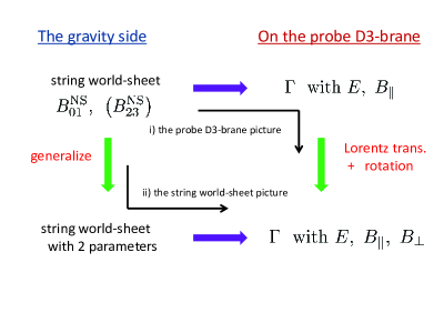
Figure 2: The two ways to introduce magnetic fields.

i) the probe D3-brane picture

The configuration of the string world-sheet in the presence of parallel electric and magnetic fields is the same as the one with the electric field only. We first suppose that there are parallel electric and magnetic fields on $x$-direction, respectively $E_{(\text{s})}$ and $B_{(\text{s})}$. By performing the Lorentz boosting in the $z$-direction, $E_{(\text{s})}$ and $B_{(\text{s})}$ are transformed as

$$E^{\prime}_{x}=E_{(\text{s})}\gamma,\qquad E^{\prime}_{y}=-B_{(\text{s})}\gamma\beta\,,\qquad B^{\prime}_{x}=B_{(\text{s})}\gamma,\qquad B^{\prime}_{y}=E_{(\text{s})}\gamma\beta\,,$$ (3.3)

where $\beta$ is the Lorentz-boost parameter and $\gamma$ is defined as $\gamma\equiv 1/\sqrt{1-\beta^{2}}$ . The rotation on the $x$-$y$ plane leads to

$$E^{\prime\prime}_{x} =E_{(\text{s})}\gamma\cos\vartheta+B_{(\text{s})}\gamma\beta\sin\vartheta,\qquad E^{\prime\prime}_{y} =E_{(\text{s})}\gamma\sin\vartheta-B_{(\text{s})}\gamma\beta\cos\vartheta\,,$$

$$B^{\prime\prime}_{x} =-E_{(\text{s})}\gamma\beta\sin\vartheta+B_{(\text{s})}\gamma\cos\vartheta,\qquad B^{\prime\prime}_{y} =E_{(\text{s})}\gamma\beta\cos\vartheta+B_{(\text{s})}\gamma\sin\vartheta\,.$$ (3.4)

Here let us impose

$$\tan\vartheta=\frac{\beta B_{(\text{s})}}{E_{(\text{s})}}\,,$$

so as to set $E^{\prime\prime}_{y}=0$ , and introduce the following notation,

$$E=E^{\prime\prime}_{x}\,,\quad B_{\parallel}=B^{\prime\prime}_{x}\,,\quad B_{\perp}=B^{\prime\prime}_{y}\,.$$

Solving about $E_{(\text{s})}$, we obtain

$$E_{(\text{s})}^{2}=\frac{1}{2}\left(E^{2}-{B_{\parallel}{}^{2}}-B_{\perp}{}^{2}+\sqrt{\left(E^{2}-B_{\parallel}{}^{2}-{B_{\perp}{}^{2}}\right)^{2}+4E^{2}B_{\parallel}{}^{2}}\,\right)\,.$$ (3.5)

Thus, from the computation of the production rate in the presence of the parallel electric and magnetic fields only, it is possible to calculate the production rate including the perpendicular magnetic field as well as the parallel electric and magnetic fields.

In the world-sheet description, we know the critical flux in the presence of the electric field only. By using this result, the critical value of the electric field in the presence of magnetic fields can be derived from the following relation,

$${\cal E}^{2}=\frac{1}{2}\left(E_{\text{c}}^{2}-{B_{\parallel}{}^{2}}-B_{\perp}{}^{2}+\sqrt{\left(E_{\text{c}}^{2}-B_{\parallel}{}^{2}-{B_{\perp}{}^{2}}\right)^{2}+4E_{\text{c}}^{2}B_{\parallel}{}^{2}}\,\right)\,.$$ (3.6)

By solving about $E_{\text{c}}$ again, $E_{\text{c}}$ is obtained as a function of ${\cal E}\,,B_{\perp}$ and $B_{\parallel}\,,$

$$E_{\text{c}}={\cal E}\sqrt{1+\frac{B_{\perp}{}^{2}}{{\cal E}^{2}+B_{\parallel}{}^{2}}}\,.$$ (3.7)

This expression agrees with the expectation from the argument on the DBI action.

As a side note, let us see the allowed range of $B_{\perp}/E$ . It depends on the presence of $B_{\parallel}$ . The Lorentz-boost parameter $\beta$ is now expressed as a function of $E\,,B_{\parallel}\,,$ and $B_{\perp}$ ,

$$\beta^{2}=\frac{E^{2}+{B_{\parallel}{}^{2}}+B_{\perp}{}^{2}-\sqrt{\left(E^{2}-B_{\parallel}{}^{2}-{B_{\perp}{}^{2}}\right)^{2}+4E^{2}B_{\parallel}{}^{2}}}{E^{2}+{B_{\parallel}{}^{2}}+B_{\perp}{}^{2}+\sqrt{\left(E^{2}-B_{\parallel}{}^{2}-{B_{\perp}{}^{2}}\right)^{2}+4E^{2}B_{\parallel}{}^{2}}}<1\,.$$ (3.8)

When $B_{\parallel}=0$ , $\beta=B_{\perp}/E$ and hence $B_{\perp}$ is always smaller than $E$ , in particular $B_{\perp}<E_{\rm c}$ . However, when $B_{\parallel}\neq 0$ , $B_{\perp}$ may be greater than $E$ . One can check it from the relation

$$\frac{B_{\perp}}{E}=\frac{E_{(\text{s})}^{2}+B_{(\text{s})}^{2}}{E_{(\text{s})}^{2}/\beta+B_{(\text{s})}^{2}\beta}\,,$$ (3.9)

and the ratio $B_{\perp}/E_{\rm c}$ can be greater than 1 depending on the values of $E_{(\text{s})}\,,B_{(\text{s})}\,,$ and $\beta$ .

By using (3.7), the production rate is given by

$$\Gamma\sim\exp\left(-\frac{\sqrt{\lambda}}{2}\left[\sqrt{\frac{{\cal E}}{E_{(\text{s})}}}-\sqrt{\frac{E_{(\text{s})}}{{\cal E}}}\;\right]^{2}\right)\,,$$ (3.10)

where $E_{(\text{s})}$ is given by (3.5).

Note that this result may be modified by magnetic fields when we take account of the one-loop contributions of $x(\tau)$ in the gauge-theory computation. It has not succeeded yet to compute the correct one-loop contributions, though some trials have been done [15, 21].

ii) the string world-sheet picture

There is another way to introduce magnetic fields. We shall persist in the gravity side, instead of relying on the probe D3-brane description. Naively thinking, the magnetic fields in the gauge-theory side are induced by turning on $B_{\it 2}$ like $B_{23}$ or $B_{31}$ in the gravity side. However, the coupling to $B_{\it 2}$ vanishes except $B_{01}$ by putting the classical solutions because $x_{2}=x_{3}=0$ . Hence one has to seek for an ingenious way to encode the information of magnetic fields into the string world-sheet.

One prescription is to generalize the classical solutions of the string world-sheet corresponding to circular Wilson loops [20] so as to depend on additional constant parameters. Such an example is given by [22]

$$x_{0}=-\frac{\ell\sqrt{1-\alpha^{2}}\cos\sigma}{\cosh\tau+\alpha\cos\sigma}\,,\quad x_{1}=\frac{\ell\sinh\tau}{\cosh\tau+\alpha\cos\sigma}\,,\quad r=L^{2}\frac{\cosh\tau+\alpha\cos\sigma}{\ell\sin\sigma}\,,$$ (3.11)

in the one-patch notation. Here the constant parameter $\alpha$ satisfies $0\leq\alpha\leq 1$ . For $0\leq\alpha<1$ , the solutions in (3.11) correspond to circular Wilson loops with the radius $\ell/\sqrt{1-\alpha^{2}}$ . This is obvious by noting the relation,

$$x_{0}^{2}+\left(x_{1}+\frac{\ell\alpha}{\sqrt{1-\alpha^{2}}}\right)^{2}+\left(\frac{L^{2}}{r}\right)^{2}=\frac{\ell^{2}}{1-\alpha^{2}}\,.$$ (3.12)

The case with $\alpha=1$ , in which the radius is divergent, corresponds to the straight line. Thus the solutions in (3.11) interpolate between circular Wilson loops and the straight Wilson line.

Using the solutions in (3.11), the NG part and the coupling to $B_{\it 2}$ in the classical string action are evaluated as, respectively,

$$S_{\text{NG}}=2n\pi T_{\text{F}}L^{2}\left(\frac{r_{0}\ell}{L^{2}\sqrt{1-\alpha^{2}}}-1\right)\,,\quad S_{B_{\it 2}}=-n\pi T_{\text{F}}B_{01}\left[\frac{\ell^{2}}{1-\alpha^{2}}-\left(\frac{L^{2}}{r_{0}}\right)^{2}\right]\,.$$ (3.13)

Then $\ell$ is determined by the boundary condition on the probe D3-brane like

$$\ell=\frac{r_{0}}{B_{01}}\sqrt{1-\alpha^{2}}\,.$$ (3.14)

On the other hand, one can read off from (3.12) that the radius $R$ of the string world-sheet on the probe D3-brane is represented by

$$R^{2}=\left(\frac{r_{0}}{B_{01}}\right)^{2}-\left(\frac{L^{2}}{r_{0}}\right)^{2}\,,$$ (3.15)

where we have used (3.14) . By using (3.15) , the classical action is evaluated as

$$S_{\text{cl}}^{(n)} =n\pi T_{\text{F}}L^{2}\left[\sqrt{\frac{r_{0}^{2}}{B_{01}L^{2}}}-\sqrt{\frac{B_{01}L^{2}}{r_{0}^{2}}}\;\right]^{2}\,.$$ (3.16)

Then the critical value is given by $B_{01}^{\rm(cr)}=r_{0}^{2}/L^{2}$ so that $S_{\text{cl}}^{(n)}=0$ and $R=0$ .

From (3.16) , one can read off the relation between $B_{01}$ and the electric field $E$ so as to reproduce the critical flux (3.2) with $B_{\parallel}=0$ as follows:

$$T_{\text{F}}B_{01}=\sqrt{E^{2}-B_{\perp}{}^{2}}\,.$$ (3.17)

This expression implies that $B_{01}$ should be identified with the Lorentz-boosted electric flux. According to this identification, the other parameters contained in the solutions (3.11) are translated in terms of the gauge-theory language like

$$\ell=\frac{m}{E}\,,\qquad\alpha=\frac{B_{\perp}}{E}\equiv\beta\,.$$ (3.18)

These relations are fixed from the consistency to (3.14) . Thus the solutions (3.11) contain the information of a magnetic field perpendicular to the electric field.

It is fair to ask how one can include a magnetic field parallel to the electric field into the classical solutions. When $B_{\parallel}\neq 0$ , it is quite natural from the above argument to identify $B_{01}$ as follows:

$$T_{\text{F}}B_{01}=\frac{1}{\sqrt{2}}\left[E^{2}-{B_{\parallel}{}^{2}}-B_{\perp}{}^{2}+\sqrt{\left(E^{2}-B_{\parallel}{}^{2}-{B_{\perp}{}^{2}}\right)^{2}+4E^{2}B_{\parallel}{}^{2}}\,\right]^{1/2}\,,$$ (3.19)

so that the critical flux agrees with the DBI result (3.2) . Note that $T_{\text{F}}B_{01}=E$ consistently when $B_{\parallel}\neq 0$ and $B_{\perp}=0$ .

According to this identification, the classical solutions in (3.11) should be modified. As is expected from the argument in the previous picture, the modification is so small that the parameter $1-\alpha^{2}$ is replaced as

$$1-\alpha^{2}\quad\longrightarrow\quad\frac{1-\alpha^{2}-\delta^{2}+\sqrt{(1-\alpha^{2}-\delta^{2})^{2}+4\delta^{2}}}{2}\,.$$ (3.20)

Then the boundary is satisfied under the following identification,

$$\delta=\frac{B_{\parallel}}{E}\,.$$ (3.21)

as well as the previous relations in (3.18) . When $\alpha=0$ , the parameter $\delta$ is irrelevant to the behavior of the classical solution. However, when $\alpha$ takes a finite value, the solution tends to describe the straight Wilson line again in the limit $\delta\to\infty$ .

4 Conclusion and discussion

We have studied the holographic Schwinger effect in the presence of electric and magnetic fields. There are two ways to turn on magnetic fields, i) the probe D3-brane picture and ii) the string world-sheet picture. In the former picture, magnetic fields both perpendicular and parallel to the electric field are activated by a Lorentz transformation and a spatial rotation. In the latter one, the classical solutions of the string world-sheet corresponding to circular Wilson loops are generalized to contain two additional parameters encoding the presence of magnetic fields.

In this note we have considered only homogeneous fields. It would be an interesting direction to investigate the case with inhomogeneous fields. The production rate in the presence of inhomogeneous fields is computed in some $U(1)$ gauge theories [23]. The remaining task is to find out the corresponding solutions of the string world-sheet.

It would also be very interesting to consider the Schwinger effect for non-abelian gauge fields [24, 25, 26] in the holographic QCD frameworks such as the Sakai-Sugimoto models [27]. Our result may find out some applications in this direction.

Acknowledgments

We would like to thank T. Kunihiro, S. Nakamura and H. Suganuma for useful discussions. The work of KY was supported by the scientific grants from the Ministry of Education, Culture, Sports, Science and Technology (MEXT) of Japan (No. 22740160). This work was also supported in part by the Grant-in-Aid for the Global COE Program “The Next Generation of Physics, Spun from Universality and Emergence” from MEXT, Japan.

References

• [1] W. Heisenberg and H. Euler, “Consequences of Dirac’s theory of positrons,” Z. Phys.  98 (1936) 714 [physics/0605038].
• [2] J. S. Schwinger, “On gauge invariance and vacuum polarization,” Phys. Rev.  82 (1951) 664.
• [3] G. V. Dunne, “New Strong-Field QED Effects at ELI: Nonperturbative Vacuum Pair Production,” Eur. Phys. J. D 55 (2009) 327 [arXiv:0812.3163 [hep-th]].
• [4] A. Ringwald, “Fundamental physics at an x-ray free electron laser,” hep-ph/0112254.
• [5] G. V. Dunne, “The Heisenberg-Euler Effective Action: 75 years on,” Int. J. Mod. Phys. A 27 (2012) 1260004 [Int. J. Mod. Phys. Conf. Ser.  14 (2012) 42] [arXiv:1202.1557 [hep-th]].
• [6] I. K. Affleck, O. Alvarez and N. S. Manton, “Pair Production At Strong Coupling In Weak External Fields,” Nucl. Phys. B 197 (1982) 509.
• [7] I. K. Affleck and N. S. Manton, “Monopole Pair Production In A Magnetic Field,” Nucl. Phys. B 194 (1982) 38.
• [8] J. M. Maldacena, “The large N limit of superconformal field theories and supergravity,” Adv. Theor. Math. Phys.  2 (1998) 231 [Int. J. Theor. Phys.  38 (1999) 1113]. [arXiv:hep-th/9711200].
• [9] S. S. Gubser, I. R. Klebanov and A. M. Polyakov, “Gauge theory correlators from non-critical string theory,” Phys. Lett. B 428 (1998) 105 [arXiv:hep-th/9802109].
• [10] E. Witten, “Anti-de Sitter space and holography,” Adv. Theor. Math. Phys.  2 (1998) 253 [arXiv:hep-th/9802150].
• [11] S. -J. Rey and J. -T. Yee, “Macroscopic strings as heavy quarks in large N gauge theory and anti-de Sitter supergravity,” Eur. Phys. J. C 22 (2001) 379 [hep-th/9803001].
• [12] J. M. Maldacena, “Wilson loops in large N field theories,” Phys. Rev. Lett.  80 (1998) 4859 [hep-th/9803002].
• [13] A. S. Gorsky, K. A. Saraikin and K. G. Selivanov, “Schwinger type processes via branes and their gravity duals,” Nucl. Phys. B 628 (2002) 270 [hep-th/0110178].
• [14] G. W. Semenoff and K. Zarembo, “Holographic Schwinger Effect,” Phys. Rev. Lett.  107 (2011) 171601 [arXiv:1109.2920 [hep-th]].
• [15] J. Ambjorn and Y. Makeenko, “Remarks on Holographic Wilson Loops and the Schwinger Effect,” Phys. Rev. D 85 (2012) 061901 [arXiv:1112.5606 [hep-th]].
• [16] S. Bolognesi, F. Kiefer and E. Rabinovici, “Comments on Critical Electric and Magnetic Fields from Holography,” JHEP 1301 (2013) 174 [arXiv:1210.4170 [hep-th]].
• [17] E. S. Fradkin and A. A. Tseytlin, “Quantum String Theory Effective Action,” Nucl. Phys. B 261 (1985) 1.
• [18] C. Bachas and M. Porrati, “Pair creation of open strings in an electric field,” Phys. Lett. B 296 (1992) 77 [hep-th/9209032].
• [19] N. Drukker, D. J. Gross and H. Ooguri, “Wilson loops and minimal surfaces,” Phys. Rev. D 60 (1999) 125006 [hep-th/9904191].
• [20] D. E. Berenstein, R. Corrado, W. Fischler and J. M. Maldacena, “The Operator product expansion for Wilson loops and surfaces in the large N limit,” Phys. Rev. D 59 (1999) 105023 [hep-th/9809188].
• [21] C. Kristjansen and Y. Makeenko, “More about One-Loop Effective Action of Open Superstring in $AdS_{5}\times S^{5}$,” JHEP 1209 (2012) 053 [arXiv:1206.5660 [hep-th]].
• [22] A. Miwa and T. Yoneya, “Holography of Wilson-loop expectation values with local operator insertions,” JHEP 0612 (2006) 060 [hep-th/0609007].
• [23] G. V. Dunne and C. Schubert, “Worldline instantons and pair production in inhomogeneous fields,” Phys. Rev. D 72 (2005) 105004 [hep-th/0507174].
• [24] A. Casher, H. Neuberger and S. Nussinov, “Chromoelectric Flux Tube Model of Particle Production,” Phys. Rev. D 20 (1979) 179.
• [25] J. Ambjorn and R. J. Hughes, “Canonical Quantization In Nonabelian Background Fields. 1.,” Annals Phys.  145 (1983) 340.
• [26] M. Gyulassy and A. Iwazaki, “Quark And Gluon Pair Production In $SU(n)$ Covariant Constant Fields,” Phys. Lett. B 165 (1985) 157.2
• [27] T. Sakai and S. Sugimoto, “Low energy hadron physics in holographic QCD,” Prog. Theor. Phys.  113 (2005) 843 [hep-th/0412141]; “More on a holographic dual of QCD,” Prog. Theor. Phys.  114 (2005) 1083 [hep-th/0507073].