Gold particle quantification in immuno-gold labelled sections for transmission electron microscopy

Abstract

We briefly outline an algorithm for accurate quantification of specific binding of gold particles to fixed biological tissue samples prepared for immuno-transmission electron microscopy (TEM). The algorithm is based on existing protocols for rational accounting of colloidal gold particles used in secondary antibodies for immuno-gold labeling.

1 Introduction

Vascular smooth muscle cells in intact tissue are the primary focus of the work done in our laboratory. Different TEM samples from the same tissue batch are usually prepared both for ultrastructural imaging and for immuno-gold labeling. The former yields, among other features, a picture of the distribution of membrane-bound components such as mitochondria, SR, lysosomes, Golgi apparatus and plasma membrane. We then perform immuno-gold labeling of ultrathin (50 to 80 nm) sections with primary antibodies typically targeting relevant transport or membrane proteins. Specifically, our laboratory is interested in various isoforms of sarco/endoplasmic reticulum ATPases (SERCA), lysosome associate membrane proteins (LAMP), ${\rm Na}^{+}/{\rm Ca}^{2+}$ exchange proteins, ryanodine receptors (RyR), and IP₃R.

2 Gold Detection Algorithm

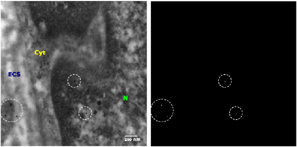
The electron micrographs produced during the imaging of tissue samples prepared for immunogold labeling typically contain faint grey-scale images of the cells, organelles and nuclei. Gold nanoparticles used for labeling appear round and very dark, with a fixed size, visible only at a magnification of 30000$\times$ or more. There may be other dark regions, usually oddly shaped, lighter than the gold, and of varying in size, that are most likely artifacts introduced in the fixing, or staining processes. Using the scripting language Python, we wrote a software algorithm for automatic detection of gold nanoparticles. It consists of three main steps, addressed in the following subsections: contrast filtering, spot detection, size filtering, and shape filtering.

2.1 Constrast filter

The contrast filter, as implemented in the Python script, is designed to sort the grayscale pixels into two categories: those that are potentially gold and those unlikely to be gold. This is based upon the observation that gold particles are significantly darker than the rest of the cell. Note that for the electron micrographs, higher density particles corresponds to a lower intensity value of the associated image pixel. Gold particles, being dense, therefore appear darker than the rest of the image.

The contrast filter uses an arbitrary intensity cut-off, anywhere from 10 to 40 out of 255, by which it is possible to retain a large percentage of the gold pixels, whilst keeping little of the background material. The higher this intensity cut-off is, the greater the percentage of gold particles that will be detected. Increasing this value does, however, also increase the amount of non-gold which passes through the filter, which in turn increases the chance of a false-positive. A right balance is struck by appropriate algorithm validation against reference images. Though the implemented version converts the image into this binary array, it would also be possible to raise the cut-off and store in the array a probability of the specified pixel being part of a gold particle. Thus, a pixel close to the cut-off would still be stored as a potential gold location, but would have less weight in the following algorithms than a pixel with a lower intensity value.

2.2 Spot detection

The spot detection portion of the algorithm detects dense areas and separates them into different regions, called spots. Two pixels lie in distinct spots if there exists no path joining the two pixels, which lies entirely within the high-density regions. Here a path represents a series of pixels which share a common edge. The algorithm works by rastering over the pixel grid generated from the contrast filter, and performing a flood-fill on every dark pixel it encounters. The flood-fill stores all the location of all the pixels in the same spot as the original pixel. Then, the region is turned white, to avoid repeating the same pixel in two distinct spots. A flood-fill algorithm is a recursive algorithm for determining all pixels which lie in a given boundary, or, as in this case, all pixels in a simply-connected region, which have the same colour. It grows by checking the neighbours of all the pixels in the current region, and, if they match the criteria, adding them to the new region. This process continues until no new additions take place between successive iterations.

2.3 Size filter

Gold particles are, by their fabrication, of constant size ($\pm 0.56$ nm) [1]. When trying to determine which of the dark spots are gold, this criterion is useful for providing a preliminary filter. In the images, apart from the problems with pixelation, all gold particles occupy roughly the same number of pixels. Thus, introducing a band pass filter on spot size guarantees that only particles close in size to gold are considered as such by the algorithm. Single pixels, which are ’round’ like gold, and large, round artifacts are eliminated at this stage in the algorithm. Since each spot is stored as a list of locations, one can easily implement this filter by simply comparing the size of this list to the expected parameters. Provided images have similar magnification and contrast, choosing these parameters need only be done once.

2.4 Shape filter

The shape filter utilizes another of the key characteristics of the gold particles: their projection onto a plane, such as what occurs when taking an electron micrograph, is a circle. In the Python script, for each spot the sum of the squared distance of each location from the spot centroid is calculated. Dividing this by the area squared gives a quantity which will be at a minimum for circles, where the value will be 1/2. Alternatively, one could use instead the eccentricity, $e$. Determining the largest and smallest distance of an edge pixel from the centroid, $r_{\rm max}$ and $r_{\rm min}$ respectively, it can be calculated using:

$$e={r_{\rm max}-r_{\rm min}\over r_{\rm max}+r_{\rm min}}$$ (1)

For a circular object, this value should be zero, with higher values corresponding to regions which have less radial symmetry. Using either method, once the quantity for comparison has been calculated, a low pass filter may be employed to eliminate any non-circular objects.

The right panel of Figure 1 shows the result of the algorithm with colours inverted for clarity.

Figure 1: Left: Electron micrograph of rat pulmonary artery stained for SERCA1 (gold particles inside dashed circles). Right: Result of gold detection algorithm applied to the image on the left. Gold is represented as white. ECS=extracellular space, Cyt=cytoplasm, N=nucleus.

3 Gold Preferential Localization Analysis

3.1 Localization ratio

The utility of the gold detection algorithm could be extended to include unbiased region and membrane localization analysis. The specificity of localization to a region M can be determined by the ratio:

$$R={G_{M}/G_{C}\over A_{M}/A_{C}}$$ (2)

where $G_{M}$ and $G_{C}$ are the number of gold particles in the region and cell respectively, and $A_{M}$ and $A_{C}$ are their areas [2]. A value of 1 corresponds to a near random distribution. A ratio higher than 1 suggests localization whilst a ratio less than 1 signifies an absence of that particle in the specified region. The farther the deviation from 1, the greater is the extent of localization to, or absence from, the region. Assuming the gold, if unlocalized, would follow a binomial distribution with probability $p=A_{M}/A_{C}$ , i. e., a uniform probability distribution over the area of the cell, the standard deviation expected would be $\sigma=\sqrt{np(1-p)}=\sqrt{G_{C}{A_{M}\over A_{C}}(1-{A_{M}\over A_{C}})}$. This can be used to test the likelihood that a given particle distribution is the product of random placement.

3.2 Membrane and region selection

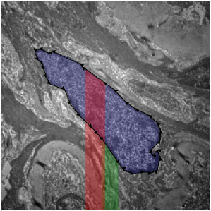
By using the counting algorithm described above, one can count the numbers of particles in specified regions and calculate the value of $R$ for various regions or membranes of interest, as identified in a computer readable format (we used the software package ‘inkscape’). This is carried by outlining the region, or membrane, of interest in a closed path. For the membrane, the ‘Halo’ function in inkscape is then used, A custom Python script was written which exports these closed paths as lists of node locations. The entire cell is also outlined, to give the whole cell area for comparison.

3.3 Area Calculation

The area of the closed region defined by a boundary path is determined by first choosing either the $x-$ or $y-$direction [3]. The program then loops through each pair of successive nodes and calculates the signed area of the trapezoid relative to that axis. Thus, if the points happen to be in reverse order relative to that axis, the trapezoid will have a negative area. The areas of all the trapezoids are summed and the resultant value is, up to a sign, the total area of the desired region. In order to deal with the area a given distance from a specified line or point, one could instead use a flood-fill algorithm which tests the distance from the line for each prospective point.

Figure 2: A stylized depiction of the operation of the area algorithm. The region shaded in blue is the area to be measured. The red trapezoid, as the arrows suggest, is one with a negative area contribution whilst the green trapezoid yields a positive contribution.

3.4 Whole Cell Analysis

If the image of the individual parts of the cell can be stitched together, then the membranes or regions can be left in place. Then, when the gold detection algorithm runs, the software can determine whether or not each gold particle is inside the region. The ratio can then be calculated for the entire cell. If stitching is not possible, then one can take a series of pictures either of the whole cell or randomly selected regions. In this case, one must then face the attendant problem of ensuring the images are a truly random sample, with a sample size large enough to ensure that enough of the desired membrane, or region is present. The distance of the gold can be determined either manually or electronically by seeing, for each picture, if any region is present, and where the gold particles are distributed relative to that region.

References

- [1] Yun Yang, Ya Yan, Wei Wang, and Jinru Li. Precise size control of hydrophobic gold nanoparticles using cooperative effect of refluxing ripening and seeding growth. Nanotechnology, 19(17):175603, Apr 2008.
- [2] Terry Mayhew, Gareth Griffiths, Anja Habermann, John Lucocq, Nil Emre, and Paul Webster. A simpler way of comparing the labelling densities of cellular compartments illustrated using data from vparp and lamp-1 immunogold labelling experiments. Histochem Cell Biol, 119(4):333–341, Apr 2003.
- [3] M.F. Goodchild and K.K. Kemp. NCGIA Core Curriculum in GIS. National Center for Geographic Information and Analysis, 1990.