Measuring the configurational temperature of a binary disc packing
Song-Chuan Zhao and Matthias Schröter∗
Jammed packings of granular materials differ from systems normally described by statistical mechanics in that they are athermal. In recent years a statistical mechanics of static granular media has emerged where the thermodynamic temperature is replaced by a configurational temperature which describes how the number of mechanically stable configurations depends on the volume. Four different methods have been suggested to measure . Three of them are computed from properties of the Voronoi volume distribution, the fourth takes into account the contact number and the global volume fraction. This paper answers two questions using experimental binary disc packings: First we test if the four methods to measure compactivity provide identical results when applied to the same dataset. We find that only two of the methods agree quantitatively. Secondly, we test if is indeed an intensive variable; this becomes true only for samples larger than roughly 200 particles. This result is shown to be due to recently measured correlations between the particle volumes [Zhao et al., Europhys. Lett., 2012, 97, 34004].
1 Is there a well defined configurational temperature?
00footnotetext: Max Planck Institute for Dynamics and Self-Organization (MPIDS), 37077 Goettingen, Germany00footnotetext: matthias.schroeter@ds.mpg.deTemperature is the concept that helps us to understand how the exchange of energy stored in the microscopic degrees of freedom follows from the accompanying change of entropy of the involved systems. If we coarse-grain our view to the macroscopic degrees of freedom of particulate systems, such as foams or granular gases, we can still define effective temperatures that describe their dynamics 1, 2. This approach defines these systems as dissipative; kinetic energy of the particles is irrecoverably lost to microscopic degrees of freedom.
In the absence of permanent external driving such system will always evolve towards a complete rest. And in the presence of boundary forces or gravity this rest state will be characterized by permanent contacts between the particles which allow for a mechanical equilibrium. Shahinpoor 3 and Kanatani 4 were the first to suggest that such systems might still be amenable to a statistical mechanics treatment. Sam Edwards and coworkers5, 6 have then developed this idea into a full statistical mechanics of static granular matter by using the ensemble of all mechanically stable states as a basis. A crucial requirement of such an approach is the existence of some type of excitation which lets the system explore the phase space of all allowed static configurations. This could e.g. be realized by tapping, cyclic shear, or flow pulses of the interstitial liquid. While there are promising results, the feasibility of this approach is still under debate 7.
A second key concept in Edwards’ approach is the replacement of the energy phase space by a volume phase space where the volume function takes the role of the the classical Hamiltonian. The configurations represent the positions and orientations of all grains. One can then define an analog to the partition function :
| (1) |
where limits the integral to mechanically stable configurations. is the configurational temperature or compactivity, which is defined as . The configurational entropy corresponds to the logarithm of the number of mechanically stable configurations for a given set of boundary condition.
is neither known from first principles (except for model systems 8, 9) nor can it be measured directly. Therefore ”thermometers” measuring have to exploit other relationships; four different ways to do so have been suggested. In this paper we will test all four of them using the same dataset of mechanically stable disc packings.
First can be determined from the steady state volume fluctuations using an analog to the relationship between specific heat and energy fluctuations 10, 11, 12, 13; we will refer to this compactivity as . A second method is based on the probability ratio of overlapping volume histograms 14, 15, allowing us to compute . A third way 16, 17 computes from Gamma function fits to the volume distribution. Finally, it has been suggested recently 18, that an analysis based on so called quadrons 19 instead of Voronoi cells leads to an expression for that involves the average particle volume and the contact number.
This difference in approach immediately raises the question if these four methods provide identical results when applied to the same experiment. There have been two previous experiments addressing this question: McNamarra et al. 15 found that and agree for tapped packings of approximately 2000 glass spheres. The same result has been reported by Puckett and Daniels 20 for compressed disc packings.
The full description of a granular packing has to take the boundary stresses into account 21, 22, 18. The stress dependence of the entropy then gives rise to a tensorial temperature named angoricity. Angoricity has been computed from numerics using the overlapping histogram method 23 and from experiments using both fluctuations and overlapping histograms 20. As the experiments described below are performed in an open cell with gentle driving, the boundary stresses can be assumed to be small and constant; we therefore exclude angoricity from our further analysis.
2 Correlations in the Voronoi-volume of disc packings
The three methods to compute , , and all start from the Voronoi-volume distribution. However, it has been shown that the Voronoi volumes inside a sample are correlated 25. We recently measured the spatial extension of this correlations and demonstrated the existence of additional anti-correlations between the volumes 24. These correlations raise the question if is indeed an intensive parameter i.e. if its value is independent of the number of particles analyzed. As the Voronoi-volumes reported in reference 24 will be the basis of this study we quickly recap the relevant experimental procedures and results, more details can be found in the original publication. The disc coordinates of all configurations and volume fractions can be downloaded from the Dryad repository 26.
2.1 Experimental setup
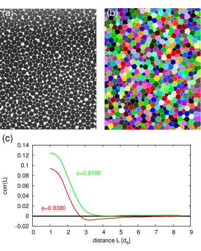
The experiment is performed in an air-fluidized bed filled with a binary mixture of Teflon discs with = 6mm and = 9 mm diameter. Data sets of 8000 different mechanically stable configurations are prepared by repeated air pulses. Changing pressure and duration of the air pulses allows us to control the average packing fractions in the ranges of 0.818 to 0.838. After each flow pulse the discs come to a complete rest and are then imaged with a CCD camera (Fig. 1 a). After detecting the particle centers, the Voronoi volume of each disc is determined (Fig. 1 b). We then compute the free volume for each particle with being the volume the grain would occupy in a hexagonal packing of identical discs. This step allows us to superimpose the results for small and large discs in the subsequent analysis.
Our results will also depend on the packing fraction of the loosest possible packing =0.811. This value is averaged over 10 packings prepared by slowly settling the discs in a manually decreased air flow.
2.2 Correlations in binary disc packings
The correlation between the Voronoi volumes can be measured using:
| (2) |
Here , are two points in the packing which separated by a distance . The free volumes at these points are and . Subtracted from them is the average free volume of all particles at this point (averaged over all 8000 taps). indicates averaging over the 8000 packings and additionally 240 pairs of points within each packing. is the variance of the free volumes averaged over the two points.
Figure 1 c) depicts for two different packing fractions. At low values of only positive correlation between Voronoi cells are found. Above = 0.8277 anti-correlations appear for larger than approximately 2.5 small particle diameters. We will show below that these (anti-) correlations control how becomes intensive.
3 Compactivity measured from volume fluctuations
This methods starts from the assumption of a Boltzmann like probability distribution:
| (3) |
From equation 3 follows for the probability to observe a certain volume at a given compactivity :
| (4) |
where the density of states counts the number of the mechanical stable states available at volume . Using equation 4 we can determine the average volume as
| (5) |
Taking the derivative of equation 5 with respect to shows that
| (6) |
on the other hand can be rewritten as from which follows:
| (7) |
Nowak et al. were the first to suggest that integrating equation 7 provides a way to compute 10:
| (8) |
where the compactivity at the loosest possible packing has been set to infinity: . First measurements 11, 12 of showed that it indeed measures a material property as it depends on the roughness of the particles. It has to be pointed out that this method has the epistemological status of a calculation rule and not of a test of the Boltzmann assumption made in equation 3. This is different for the overlapping histogram method described below.
As described in section 2 we are interested in the evolution of with the size of the analyzed region, in the following referred to as cluster. Therefore we continue our study by using the normalized average volume per particle where the sum goes over all particles inside the cluster, is the Voronoi volume of the individual particles and the volume occupied by the particle itself. As a consequence of this choice also is dimensionless.
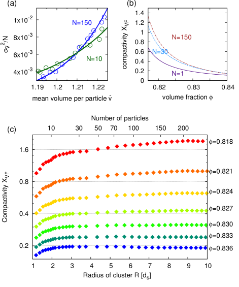
Figure 2 (a) shows that for our tapped disc packings the variance of the volume fluctuation increases monotonically with the average volume (bar meaning again the average over all 8000 taps). To compute we perform a power law fit to and use the result to integrate equation 8 numerically. Figure 2 (b) shows how the resulting depends on the packing fraction at cluster sizes of 1, 30, and 150 discs. It is obvious that is not an intensive variable for this range of .
3.1 Correlations make non-intensive in small systems
For a more detailed analysis we have plotted in figure 2(c) the dependence of on the cluster radius measured in small disc diameters . Three features of become apparent:
-
1.
is growing monotonously for for all values of ,
-
2.
for low to intermediate values of , then reaches a plateau, and
-
3.
for the highest packing fraction first decreases slightly before entering a plateau.
All three points can be understood by considering the influence of the volume correlations shown in figure 1. Equation 8 computes from the average variance inside the cluster. This variance can be decomposed in the following way:
| (9) |
Here is the fluctuation of a single Voronoi cell and is the volume correlation between disc and all other discs inside the cluster. If is in the center of the cluster, then is proportional to the area enclosed by , the zero line, and in figure 1(c).
This consideration allows us to explain feature 1: while goes from 2 to approximately 25 all are positive and growing. Consequentially, the variance of the cluster is larger than the sum of the variance of the individual Voronoi cells and grows monotonously with .
The second feature stems from the fact, that once disk is more than four to five away from the boundary of the cluster, becomes independent of the cluster size. As the relative importance of ”boundary discs” decreases with cluster size, goes to a constant and becomes independent of .
Finally, the slight decrease in at high packing fractions and values between approximately 30 and 150 can be attributed to the anti-correlations that appear for larger than 0.8277; these will decrease slightly again before it reaches its plateau value.
4 Compactivity measured from overlapping histograms
This way to compute compactivity has been first described by Dean and Lefèvre 14. It uses pairs of experiments with slightly different values of respectively and computes then the ratio of the probabilities to observe the same local volume . If the assumption of a Boltzmann-like probability distribution, as expressed in equation 4, holds, this ratio should be exponential in :
| (10) |
By taking the logarithm on both sides we obtain:
| (11) |
Therefore the difference between two compactivities can be computed from a line fit of versus as it was first demonstrated in 15.
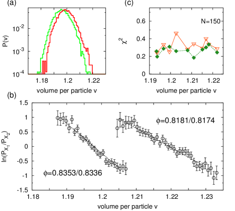
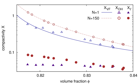
Figure 3(a) shows the distribution of average volumes for two experiments with a packing fraction difference of 0.0017. Figure 3(b) demonstrates that the ratio is indeed a linear function of , as predicted by equation 11. By sweeping the experimentally accessible range of packing fractions, can be determined from the accumulated compactivity differences up to an additive constant . We determine by setting for the loosest experimental packing to the value of at this volume fraction.
The resulting is shown in figure 4. The good quantitative agreement of and is not too surprising given that a) both methods are derived from the same probability distribution (equation 4) and b) our determination of . However, the method provides an additional test of the assumptions leading to equation 4 as we can compare the quality of a linear fit to with fit functions derived from alternative probability distribution functions 15. A generic candidate would be a Gaussian distribution which results in parabolic fit. Figure 3(c) demonstrates however that a linear fit is superior, adding credibility to a Boltzmann-like approach. Also note that canceling the density of states in equation 10 implicitly assumes a weak form of ergodicity; if the system explores its phase space differently at the two values of we can’t eliminate .
5 Compactivity measured from a Gamma distribution fit
This third method to compute compactivity has been suggested by Aste and Di Matteo 17, 27; it differs from the previous approaches that it explicitly determines the density of states . Based on the observation 16 that experimental Voronoi volume distributions can be well fit by distributions, they propose to replace equation 4 with a rescaled distribution
| (12) |
where is the mean free volume (as defined in section 2), and is the shape factor. They then identify
| (13) |
or by making use of the fact that variance of the function is given by: they derive
| (14) |
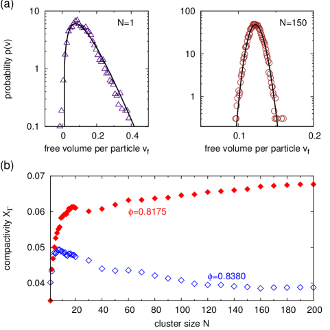
Figure 5 (a) demonstrates that our volume distribution is well fit by a distribution. We then determine without any additive constant using equation 14. Figure 4 show in comparison to and . While all three compactivities decrease monotonously with , the absolute values and the slope of are quite different from and .
Figure 5 (b) shows the evolution of with cluster size. A comparison with , displayed figure 2 (c), shows a qualitative similar influence of the volume correlations: while increases towards a plateau for small values of phi, it goes through a maximum before reaching a smaller plateau value for the densest packings.
6 Compactivity measured from quadron tessellation
In a recent paper Blumenfeld et al. 18 presented an analysis of the statistical mechanics of two-dimensional packings based on quadrons 19 as the building blocks of the tessellation. An advantage of this choice is that the quadrons take by design into account the structural degrees of freedom of the individual particles. A drawback is that quadrons are not necessarily volume conserving in the presence of non-convex voids formed by ”rattlers”, i.e. particles lying at the bottom of larger voids. 28, 29. Blumenfeld and coworkers then derive the partition functions of the volume ensemble , the force ensemble , and the total partition function , showing in this process that . Finally, they obtain from an expression for of an isostatic packing:
| (16) |
is the average volume of a cluster, the average number of contact a particle has, and is the number of boundary forces.
If is derived from instead of one obtains:
| (17) |

In comparing our results with this approach we have to acknowledge two differences. First, our experimental packings are clearly subject to volume forces due to gravity. And secondly they are, as shown in figure 6 (a), hyperstatic, i.e. their contact number is larger than what is required to fix all their mechanical degrees of freedom.
Generally, frictional particles only become isostatic at Random Loose Packing and zero pressure 30, 31. Therefore the only direct comparison possible is at our RLP value = 0.811, the corresponding is shown as black circle in figure 6 (c). If we assume that we can replace in equation 16 with and use the contact numbers displayed in figure 6 (a), we can also compute for a larger range of . These results are indicated as the open squares in figure 6 (c).
As is only computed from the average volume of a cluster, it is insensitive to the correlations described in section 2. On the other hand there exists a finite size effect if is computed from the volume ensemble, ignoring the boundary forces. Figure 6 (b) shows how the difference between the compactivities computed from the full and the volume ensemble vanishes with increasing cluster size and consequentially decreasing contribution of .
7 Which is the correct way to measure compactivity?
Figures 4 and 6 (c) show clearly that the four different methods to compute compactivity do not agree quantitatively. While and are identical within experimental scatter, is more than one order of magnitude smaller than and and at the same time decreasing less steeply with volume fraction32. The values of are closer to and again, but the evolution with is similar to .
Our data can be used to self-consistently compute all four different versions of compactivity, consequentially they are unsuitable as a basis to judge the correctness of the different approaches. A potential experimental or numerical test would need an independent determination of the compactivity of a model system from the knowledge of its entropy as a function of volume. Alternatively, if the granular statistical mechanics could be advanced to make predictions of granular behavior (e.g. segregation 33) based on specific values of , these could be tested versus the four different ”thermometers”.
However, we can elucidate the difference between the four methods by computing the density of states and comparing it to what is known to about RLP, the loosest possible, mechanically stable packing.
7.1 Computing the density of states
A probability distribution of the type of equation 3 is a generic feature for every statistic theory that maximizes the amount of entropy represented by , given certain constraints 34. In this spirit the density of states in equation 4 can be interpreted as encapsulating the physics of the specific system under consideration, while the exponential term represents our lack of knowledge about the microscopic state. From this perspective the main difference between the four methods is the way they determine : while and treat it as an experimental input parameter, and do provide predictions for its dependence on . In this subsection we will however not discuss as the theory has not been expanded yet to hyperstatic packings.
can be computed following McNamara et al 15. Starting by rewriting equation 4 to
| (18) |
we remove the dependence on the unknown partition function by taking the ratio with at a given volume :
| (19) |
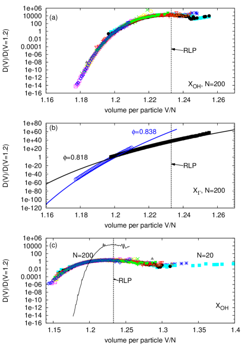
The results are presented in figure 7 where we have chosen = 1.2. Panel (a) shows that the density of states ratios computed from all eleven values of overlap, as it can be expected if the different preparation protocols sample the phase space with the same probabilities. Figure 7 (b) shows that this agreement of the density of states is not obtained if the ratio is computed from .
Figure 7 provides also some insight how the configurational entropy depends on on the volume:
| (20) |
where is the equivalent to the Boltzmann constant. As our system is large enough and not constrained by boundaries (for a counter example see 35), we obtain a smooth function and can therefore choose the integration interval small enough so that its contribution to vanishes.
7.2 Random Loose Packing
Random Loose Packing (RLP) is first of all defined phenomenologically as the loosest possible packing which is still mechanically stable, i.e. has a finite yield stress. Mechanical stability requires the packing to be at least isostatic: the average number of contacts of a particle needs to be large enough to provide sufficient constraints to fix all its degrees of freedom 30, 36, 31. Experimentally it has been found that of spheres is approximately 0.55 37, 38, 39 with the precise value depending on the friction coefficient 38, 39 and the confining pressure38. For binary disc packings does also depend on their diameter ratio; for the particles in this paper we measured = 0.811.
While RLP seems to imply that there exist no packings with lower , exactly such states have been identified in MD simulations with = 20 discs; the new lower boundary where such states vanish has been named Random Very Loose Packing (RVLP) 40. An explanation why these states between RLP and RVLP are usually not observed in experiment is given by their small basin of attraction in phase space.
In general, the statistical mechanics approaches to granular media5, 6, 7 assume the configurational temperature . Then it follows from
| (21) |
that the configurational entropy increases the looser the packings become. At RLP reaches a maximum and then decays to zero for looser configurations which by definition are not mechanically stable packings. Further on, it is often assumed that the maximum of S is analytic which implies that becomes infinity at RLP5, 6, 40.
The density of states computed from respectively does agree with these predictions; figure 7 shows that it reaches a global maximum at RLP. This is however only a self-consistency test as the value of explicitly entered the computation of these two compactivities. More probative is the fact that the volume fluctuations used to compute have been shown to depend on 11. Consequentially, also a configurational entropy computed from will depend on , which is a necessary condition as the number of mechanically stable configurations is also depending on .
Figure 7 c) shows that the density of states does also depend on the size of the system. Systems with 20 discs posses considerably looser states than those with 200 discs. This effect points to an explanation of the configurations between RLP and RVLP as a consequence of the finite size of a system, they will vanish in the thermodynamic limit.
The density of states computed from (figure 7 b) seems not to display a maximum at . However, RLP might become the most likely state if in the limit the states between RLP and RVLP vanish. Either way, will be finite and display a jump to approximately half its value for the ”fluid” configurations below 27, which have Voronoi volume distributions that are also well described by Gamma functions41. While this behavior might be not the canonical expectation, especially as is undefined for fluid, non-stable configurations, it does not contradict experimental results. This is different for the influence of friction: it has been shown that the Gamma distribution fits are independent of 16, 17, consequentially neither , nor and the derived will reflect the different number of mechanical stable states resulting from changes in friction.
Finally, it is difficult to comment on the relationship between and RLP as the theory is presently only worked out at exactly RLP. is of finite value and will depend only very weakly on via . If we allow similar to for its existence also for , will be depending on the preparation protocol because the contact number is protocol dependent below RLP42.
7.3 Open questions
Because granular matter is athermal, the question of ergodicity has to be answered separately for each experimental or numerical protocol used to explore the phase space of mechanically stable configurations. An indication of their differences is e.g. the different dependence of the volume fluctuations when the sample is either mechanically tapped12 or excited by flow pulses11. Nonergodicity has recently also been shown for numerical tapping of frictionless hard spheres43, however there the analysis was not restricted to mechanically stable states. In contrast, in numerical simulations of frictional discs fluidized with flow pulses an equivalence between time and ensemble averages has been found44.
The biggest challenge to the concept of a configurational granular temperature are however recent experiments by Puckett and Daniels20 where they studied the volume and force fluctuations of two samples of discs which where in mechanical contact. They found that the angoricity of the two samples equilibrated, but the compactivity (computed as and ) did not. However, their preparation protocol was biaxial compression which did not allow for strong particle rearrangements, therefore it might have been prohibiting volume exchange between the two subsystems by quenching too fast. Clearly more work is needed to answer the question if compactivity is a variable predictive of granular behavior or just a number following from an algorithm.
8 Conclusions
Using the same experimental dataset, we have computed the configurational granular temperature with the four different methods that have been previously suggested. The two methods that treat the density of states as an experimental input agree quantitatively with each other. The values computed from the other two methods, which specify the density of states from independent theoretical considerations, are both different from each other and from the first two methods. Our results do not provide a direct way to judge the correctness of the individual approaches. But the derived density of states shows that only the two agreeing methods provide a satisfying explanation how Random Loose Packing depends on friction.
Our measurements also demonstrate that becomes only an intensive variable when computed for clusters of size larger 150 particles. This effect is due to the volume correlations of neighboring particles. Consequentially, individual Voronoi cells are not suitable ‘quasi-particles’ to define a configurational temperature in granular packings. This will complicate the application of a statistical mechanics approach to small granular systems and in the presence of local gradients.
We acknowledge helpful discussions with Karen Daniels and Klaus Kassner.
References
- 1 Ian K. Ono, Corey S. O’Hern, D. J. Durian, Stephen A. Langer, Andrea J. Liu, and Sidney R. Nagel. Effective temperatures of a driven system near jamming. Phys. Rev. Lett., 89:095703, 2002.
- 2 N. V. Brilliantov and T. Pöschel. Kinetic Theory of Granular Gases. Oxford University Press, 2004.
- 3 M. Shahinpoor. Statistical mechanical considerations on the random packing of granular materials. Powder Technology, 25:163–176, 1980.
- 4 Ken-Ichi Kanatani. The use of entropy in the description of granular materials. Powder Technology, 30:217–223, 1981.
- 5 S.F. Edwards and R.B.S. Oakeshott. Theory of powders. Physica A, 157:1080–1090, 1989.
- 6 Anita Mehta and S. F. Edwards. Statistical and theoretical physics : Statistical mechanics of powder mixtures. Physica A, 157:1091–1100, 1989.
- 7 Massimo Pica Ciamarra, Patrick Richard, Matthias Schröter, and Brian P. Tighe. Statistical mechanics for static granular media: open questions. Soft Matter, 8:9731, 2012.
- 8 R. Monasson and O. Pouliquen. Entropy of particle packings: An illustration on a toy model. Physica A, 236:395–410, 1997.
- 9 Richard K. Bowles and S. S. Ashwin. Edwards entropy and compactivity in a model of granular matter. Physical Review E, 83:031302, 2011.
- 10 Edmund R. Nowak, James B. Knight, Eli Ben-Naim, Heinrich M. Jaeger, and Sidney R. Nagel. Density fluctuations in vibrated granular materials. Phys. Rev. E, 57:1971–1982, 1998.
- 11 Matthias Schröter, Daniel I. Goldman, and Harry L. Swinney. Stationary state volume fluctuations in a granular medium. Phys. Rev. E, 71:030301, 2005.
- 12 Ph. Ribière, P. Richard, P. Philippe, D. Bideau, and R. Delannay. On the existence of stationary states during granular compaction. Europ. Phys. J. E, 22:249 – 253, 2007.
- 13 Christopher Briscoe, Chaoming Song, Ping Wang, and Hernan A. Makse. Entropy of jammed matter. Physical Review Letters, 101:188001–4, 2008.
- 14 David S. Dean and Alexandre Lefèvre. Possible test of the thermodynamic approach to granular media. Phys. Rev. Lett., 90:198301, 2003.
- 15 Sean McNamara, Patrick Richard, Sébastien Kiesgen de Richter, Gérard Le Caër, and Renaud Delannay. Measurement of granular entropy. Phys. Rev. E, 80:031301, 2009.
- 16 T Aste, T. Di Matteo, M Saadatfar, T. J Senden, Matthias Schröter, and Harry L Swinney. An invariant distribution in static granular media. EPL, 79:24003, 2007.
- 17 T. Aste and T. Di Matteo. Emergence of gamma distributions in granular materials and packing models. Phys. Rev. E, 77:021309, 2008.
- 18 Raphael Blumenfeld, Joe F. Jordan, and Sam F. Edwards. Interdependence of the volume and stress ensembles and equipartition in statistical mechanics of granular systems. Physical Review Letters, 109:238001, 2012.
- 19 Raphael Blumenfeld and Sam F. Edwards. Granular entropy: Explicit calculations for planar assemblies. Physical Review Letters, 90:114303, 2003.
- 20 James G. Puckett and Karen E. Daniels. Equilibrating temperaturelike variables in jammed granular subsystems. Physical Review Letters, 110:058001, 2013.
- 21 Kun Wang, Chaoming Song, Ping Wang, and Hernán A. Makse. Angoricity and compactivity describe the jamming transition in soft particulate matter. Europhysics Letters, 91:68001, 2010.
- 22 Luis Ariel Pugnaloni, José Damas, Iker Zuriguel, and Diego Maza. Master curves for the stress tensor invariants in stationary states of static granular beds. implications for the thermodynamic phase space. Papers in Physics, 3:030004, 2011.
- 23 Silke Henkes, Corey S. O’Hern, and Bulbul Chakraborty. Entropy and temperature of a static granular assembly: An ab initio approach. Physical Review Letters, 99:038002, 2007.
- 24 Song-Chuan Zhao, Stacy Sidle, Harry L. Swinney, and Matthias Schröter. Correlation between voronoi volumes in disc packings. EPL, 97:34004, 2012.
- 25 F Lechenault, F da Cruz, O Dauchot, and E Bertin. Free volume distributions and compactivity measurement in a bidimensional granular packing. J. Stat. Mech., 2006:P07009–P07009, 2006.
- 26 DOI from Dryad; data upload is only possible after paper is accepted by a journal.
- 27 T. Aste and T. Di Matteo. Structural transitions in granular packs: statistical mechanics and statistical geometry investigations. The European Physical Journal B, 64:511–517, 2008.
- 28 Massimo Pica Ciamarra. Comment on granular entropy: Explicit calculations for planar assemblies. Physical Review Letters, 99:089401, 2007.
- 29 Raphael Blumenfeld and Sam F. Edwards. Blumenfeld and edwards reply:. Phys. Rev. Lett., 99:089402, 2007.
- 30 Kostya Shundyak, Martin van Hecke, and Wim van Saarloos. Force mobilization and generalized isostaticity in jammed packings of frictional grains. Phys. Rev. E, 75:010301(R), 2007.
- 31 S. Henkes, M. van Hecke, and W. van Saarloos. Critical jamming of frictional grains in the generalized isostaticity picture. EPL, 90:14003, 2010.
- 32 This difference can not be attributed to the use of the free volume for the computation of as differs from only by a constant . Therefore neither the shape of the probability distributions used to compute nor the size of the volume fluctuations, on which is based on, would change if they were also computed from .
- 33 Matthias Schröter and Karen E. Daniels. Granular segregation in dense systems: the role of statistical mechanics and entropy. arxiv.org/abs/1206.4101, 2012.
- 34 E. T. Jaynes. Information theory and statistical mechanics. Physical Review, 106:620–630, 1957.
- 35 Guo-Jie Gao, Jerzy Bławzdziewicz, and Corey S. O’Hern. Frequency distribution of mechanically stable disk packings. Physical Review E, 74:061304, 2006.
- 36 Chaoming Song, Ping Wang, and Hernán A. Makse. A phase diagram for jammed matter. Nature, 453:629–632, 2008.
- 37 George Y. Onoda and Eric G. Liniger. Random loose packings of uniform spheres and the dilatancy onset. Phys. Rev. Lett., 64:2727–2730, 1990.
- 38 Melissa Jerkins, Matthias Schröter, Harry L. Swinney, Tim J. Senden, Mohammad Saadatfar, and Tomaso Aste. Onset of mechanical stability in random packings of frictional spheres. Phys. Rev. Lett., 101:018301, 2008.
- 39 Greg R. Farrell, K. Michael Martini, and Narayanan Menon. Loose packings of frictional spheres. Soft Matter, 6:2925–2930, 2010.
- 40 Massimo Pica Ciamarra and Antonio Coniglio. Random very loose packings. Physical Review Letters, 101:128001, 2008.
- 41 V. Senthil Kumar and V. Kumaran. Voronoi cell volume distribution and configurational entropy of hard-spheres. The Journal of Chemical Physics, 123(11):114501–114501–13, 2005.
- 42 Claus Heussinger and Jean-Louis Barrat. Jamming transition as probed by quasistatic shear flow. Physical Review Letters, 102:218303, 2009.
- 43 Fabien Paillusson and Daan Frenkel. Probing ergodicity in granular matter. Physical Review Letters, 109:208001, 2012.
- 44 M. Pica Ciamarra, A. Coniglio, and M. Nicodemi. Thermodynamics and statistical mechanics of dense granular media. Physical Review Letters, 97:158001, 2006.