A Scalable Generative Graph Model
with Community Structure

Abstract

Network data is ubiquitous and growing, yet we lack realistic generative network models that can be calibrated to match real-world data. The recently proposed Block Two-Level Erdős-Rényi (BTER) model can be tuned to capture two fundamental properties: degree distribution and clustering coefficients. The latter is particularly important for reproducing graphs with community structure, such as social networks. In this paper, we compare BTER to other scalable models and show that it gives a better fit to real data. We provide a scalable implementation that requires only O($d_{{\rm max}}$) storage where $d_{{\rm max}}$ is the maximum number of neighbors for a single node. The generator is trivially parallelizable, and we show results for a Hadoop MapReduce implementation for a modeling a real-world web graph with over 4.6 billion edges. We propose that the BTER model can be used as a graph generator for benchmarking purposes and provide idealized degree distributions and clustering coefficient profiles that can be tuned for user specifications.

1 Introduction

Network interaction data are now available from online social interactions, computer-to-computer communications, financial transactions, collaboration networks, telecommunications, and more. A major obstacle to working in the field of network science is that access to data is restricted due to a combination of security and privacy concerns; yet models, algorithms, software, and hardware are struggling to keep pace with increasing demands for scalability and relevance. For these reasons, network science researchers need scalable generative models for large-scale graphs. Ideally, these generative models should capture salient features of the networks being modeled.

Suppose we are given a graph representation of our data set. We introduce basic terminology for those unfamiliar with graph theory. Let $G=(V,E)$ be an undirected, unweighted graph. We let $V$ denote the set of vertices or nodes of the graph, and we let $E$ denote the set of edges where $(i,j)\in E$ means there is an edge between nodes $i$ and $j$ or, equivalently, that nodes $i$ and $j$ are adjacent. We assume that the graph is simple, meaning that the edges and undirected and unweighted and that there are no self-edges. Let $V_{i}=\set{j}{(i,j)\in E}$ denote the set of nodes that are adjacent to $i$ then the degree of node $i$ is $d_{i}=|V_{i}|$. The transitivity or clustering coefficient of node $i$ is defined as $c_{i}=|\set{(j,k)\in E}{j,k\in V_{i}}|/\binom{d_{i}}{2}$, and it is a measure of the proportion of triangles that node $i$ participates in compared to the number of possible triangles [47]. Roughly speaking, $c_{i}$ captures the social cohesion around node $i$; for instance, in a clique (i.e., a graph in which every node is adjacent to every other node), every node has $c_{i}=1$.

In this paper, we consider how to reproduce two fundamental properties of graphs: the degree distribution and the clustering coefficients by degree [46]. Let $V_{d}=\set{i}{d_{i}=d}$ be the set of nodes of degree $d$ and define $n_{d}=|V_{d}|$. The degree distribution is specified by the sequence $\set{n_{d}}_{d\in\mathbb{N}}$. In most real-world networks representing interaction data, there are a few nodes with high degrees and many nodes with low degrees, with a smooth transition between. In other words, the degree distribution is heavy-tailed, and this feature has long been considered critical in distinguishing real networks from arbitrary sparse networks [2, 13, 41]. Let $c_{d}=\frac{1}{n_{d}}\sum_{i\in V_{d}}c_{i}$ be the average clustering coefficient for nodes of degree $d$. The clustering coefficients by degree are specified by the sequence $\set{c_{d}}_{d\in\mathbb{N}}$. The clustering coefficients of real-world graphs are much higher than those of random graphs with the same degree distribution [18]. Nonetheless, most generative models fail to match clustering coefficients of real-world graphs [40].

In previous work by a subset of the authors, we introduce the Block Two-Level Erdős–Rényi (BTER) [42]. The BTER model can be tuned to capture both the degree distribution and degree-wise clustering coefficients for real-world networks. The inputs to the BTER model are the sequences $\set{n_{d}}_{d\in\mathbb{N}}$ and $\set{c_{d}}_{d\in\mathbb{N}}$; our goal is to create a graph with similar behavior in these measures. To do this, BTER works as follows. The nodes are divided into affinity blocks; see Figure 1a. The fact that we can infer community structure from local clustering coefficient measurements is justified in the original BTER paper [42] and now has additional theoretical justification since it has recently been shown that triangle-rich graphs resemble unions of dense blocks [21]. Each node has an assigned degree in such a way that, in expectation, the degree distribution matches what it specified by $\set{n_{d}}_{d\in\mathbb{N}}$. For each node, the links are divided between local links within the affinity block (Phase 1 in Figure 1b) and global links that may connect to any node (Phase 2 in Figure 1c). The proportion of local links depends on the clustering coefficients specified by $\set{c_{d}}_{d\in\mathbb{N}}$. Edges are generated by choosing endpoints in a probabilistic way, as is explained in detail further on. The goal of this paper is to explain the specifics of the model and provide a scalable implementation. We also provide additional evidence of the model’s usefulness.

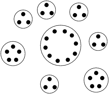
(a) Preprocessing: Distribution of nodes into affinity blocks

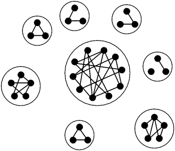
(b) Phase 1: Local links within each affinity block

(c) Phase 2: Global links across affinity blocks

Fig. 1: BTER model phases [42].

1.1 Contributions

The BTER model [42] was previously introduced as a scalable model that can reproduce degree distributions and clustering coefficients. The scalability is based on independent edge generation; i.e., there is no knowledge of previously-generated edges in deciding on the next edge. However, the original paper [42] did not specify implementation details and moreover recommended an ad hoc procedure for some of the parameter choices. In this paper, we make the following contributions:

• We provide a detailed reference implementation that clearly explains how to choose the BTER parameters to match the specified degree distribution and clustering coefficient profile. We note that there is no iterative optimization to fit BTER; the parameters of the model are directly calculated from the inputs. The edges are generated independently and in an arbitrary order, so the BTER generative model can potentially be used in streaming scenarios.

• We present efficient data structures for a scalable implementation, requiring only $O(d_{{\rm max}})$ storage and $O(\log d_{{\rm max}})$ operations per edge, where $d_{{\rm max}}$ is the maximum degree. Since our approach generates all edges independently, it can be easily parallelized. We provide examples demonstrating the scalability.

• We demonstrate that BTER gives good approximations to the degree distributions and clustering coefficient behaviors of several large, heavy-tailed, real-world graphs. We consider examples from the Laboratory for Web Algorithms [49], including a graph with over 130 million nodes and 4.6 billion edges, the largest publicly available graph that we are aware of. We also compare BTER to competing methods on a pair of smaller graphs.

• We also consider how BTER may be used for arbitrary benchmarking purposes, when there is no target graph to match. Since the model requires a degree distribution and clustering coefficient profile as input, we focus on how to generate these. In particular, we recommend the generalized log-normal distribution for the degrees as an alternative to the standard power law.

For very large graphs, the inputs can be expensive to compute, especially the clustering coefficients. However, we have recently proposed a sampling method that scales to very large graphs [44, 24].

1.2 Related Work

Since the goal of this paper is to focus on the implementation and scalability of BTER, we limit our discussion to the most salient related models. A more thorough discussion of related work can be found in the paper that originally proposed the BTER model [42].

The majority of graph models add edges one at a time in a way that each random edge influences the formation of future edges, making them inherently serial and therefore unscalable. The classic example is Preferential Attachment [2], but there are a variety of related models, e.g., [25, 28]. These models are more focused on capturing qualitative properties of graphs and typically are difficult to match to real-world data [40]. Perhaps the most relevant is [20], which creates a graph with power law degree distribution and then “rewires” it to improve the clustering coefficients. The Musketeer model starts with a given graph and then does multilevel rewiring to attempt to preserve certain features of the original [22]. Another related model, the clustering model proposed by Newman [37], assigns “individuals” to “groups” (a bipartite graph with individual and group nodes) and then creates a graph of connections between individuals by assigning connection probabilities to each group; in other words, each group is modeled as an Erdős–Rényi graph.

A widely used model for modeling large-scale graphs is the Stochastic Kronecker Graph (SKG) model, also known as R-MAT [8, 27]. The generation process is easily parallelized and can scale to very large graphs. Notably, SKG has been selected as the generator for the Graph 500 Supercomputer Benchmark [48] and has been used in a variety of other studies [14, 30, 33, 32, 19, 15, 31, 23]. Unfortunately, SKG has some drawbacks. (1) SKG can be extremely expensive to fit to real data (using KronFit, the SKG parameter fitting algorithm proposed by the SKG inventors), and even then the fit is imperfect [27]. (2) It can generate only lognormal tails (after suitable addition of random noise) [45, 43], limiting the degree distributions that it can capture. (3) Most importantly, SKG rarely closes wedges so the clustering coefficients are much smaller than what is produced in real data [40, 24].

Another model of relevance is the Chung-Lu (CL) model [10, 11, 1]. It is very similar to the edge-configuration model of Newman et al. [36]. Let $d_{i}$ denote the desired degree for node $i$. In the Chung-Lu model, the probability of an edge is proportional to the product of the degrees of its endpoints, i.e., the probability of edge $(i,j)$ is $\propto d_{i}d_{j}$. Edges can be generated independently by picking endpoints proportional to their desired degrees. If all degrees are the same, Chung-Lu reduces to the well-known Erdős–Rényi model [16]. The Chung-Lu model is often used as a null model; for example, it is the basis of the modularity metric [38]. Graphs generated by the Chung-Lu model and the SKG model are, in fact, very similar [39]. The advantage of the Chung-Lu model is that it can be better tuned to real-world degree distributions. The disadvantage of the model is that, like SKG, it rarely closes wedges. Chung-Lu occurs as a special case of BTER when Phase 1 is skipped (see §3). The Chung-Lu construction is a very important part of BTER and will be explained in more detail in the next section.

2 Notation and background

Let $G=(V,E)$ be an undirected and unweighted graph, where $V$ denotes the set of vertices and $E$ denotes the set of edges. We let $n=|V|$ and $m=|E|$ denote the total number of vertices and edges, respectively. The set of node $i$’s neighbors and the degree of node $i$ are, respectively,

$$V_{i}\equiv\set{j}{(i,j)\in E}\quad\text{and}\quad d_{i}=|V_{i}|.$$

The set of degree-$d$ nodes and the number of degree-$d$ nodes are, respectively,

$$V_{d}=\set{i}{d_{i}=d}\quad\text{and}\quad n_{d}=|V_{d}|.$$

The set $\set{n_{d}}$ defines the degree distribution. Observe that the degree distribution specifies the total number of nodes and edges:

$$n=\sum_{d}n_{d}\quad\text{and}\quad m=\frac{1}{2}\sum_{d}d\cdot n_{d}.$$ (1)

For convenience, we use the notation $d_{{\rm max}}=\max\set{d_{i}}{i\in V}$.

2.1 Clustering coefficients

We can discuss clustering coefficients in terms of wedges, closed wedges, and triangles. A wedge is a path of length 2. Figure 2 shows a wedge centered at node $j$, i.e., the path $i$-$j$-$k$ is a wedge. We say wedge $i$-$j$-$k$ is closed if $(i,k)\in E$; otherwise, the wedge is called open. A closed wedge forms a triangle, i.e., a three-cycle.

Fig. 2: Wedge centered at node $j$. The wedge is closed if $(i,k)\in E$.

The number of wedges centered at node $i$ is $\binom{d_{i}}{2}=d_{i}(d_{i}-1)/2$. The clustering coefficient at node $i$ is

$$c_{i}=\frac{\text{\# of closed wedges centered at node $i$}}{\text{\# wedges centered at node $i$}}=\frac{|\set{(j,k)\in E}{j,k\in V(i)}|}{\binom{d_{i}}{2}}.$$

This is the proportion of closed wedges divided by the total number of wedges. For BTER, we are specifically interested in clustering coefficient per degree [47], defined as

$$c_{d}=\frac{\text{\# of closed wedges centered at a node of degree $d$}}{\text{\# wedges centered at a node of degree $d$}}=\frac{1}{n_{d}}\sum_{i\in V_{d}}c_{i}.$$

To summarize an entire graph, it is often convenient to consider the global clustering coefficient (GCC) [47, 3] , defined as

$$c=\frac{\text{\# of closed wedges}}{\text{\# wedges}}.$$

Note that this is not the mean of the $c_{i}$’s. Since every triangle corresponds to three closed wedges, the number of closed wedges is three times the number of triangles.

2.2 Erdős–Rényi Graphs

As described in §3, BTER uses Erdős–Rényi to model its affinity blocks. An Erdős–Rényi graph [16] on $n$ vertices with connection probability $\rho$ is a graph such that each pair of vertices is independently connected with probability $\rho$. We refer to $\rho$ as the connectivity. If $\rho$ is a constant, we call this a dense Erdős–Rényi graph; if $\rho=O(1/n)$, then we call this a sparse Erdős–Rényi graph.

2.3 Chung-Lu Graphs

BTER uses a variation on Chung-Lu for its global links that span across affinity blocks. Here we explain salient details that are relevant to the implementation discussion.

The Chung-Lu model [10, 11, 1] approximates the probability that edge $(i,j)$ exists by

$$\text{Pr}\left((i,j)\in E\right)=\frac{d_{i}d_{j}}{2m},$$

where $d_{i}$ indicates the desired degree of node $i$. We can perform an independent coin flip for each of the possible $n^{2}$ edges, but this is too expensive. We consider a “fast” version of the Chung-Lu model that generates edges by choosing endpoints independently, proportional to their degrees. Rather than doing an independent coin flip for each of $n^{2}$ possible edges, we can do $2m$ coin flips to pick two random endpoints per edge. Each endpoint is picked independently such that the probability of picking node $i$ is

$$\text{Pr}\left(i\right)=d_{i}/2m.$$

Hence, the probability (or, more precisely, the expected value) of edge $(i,j)$ after picking $m$ edges is

$$\text{Pr}\left((i,j)\in E\right)=m\cdot 2\cdot\text{Pr}\left(i\right)\cdot\text{Pr}\left(j\right)=\frac{d_{i}d_{j}}{2m}.$$

The factor of 2 is because $(i,j)$ and $(j,i)$ are equivalent for an undirected graph.

Let $D_{i}$ correspond to the random variable that is the degree of node $i$ for a single graph generated according to this procedure. In the “fast” version, it is easy to see that the value of $D_{i}$ is Poisson distributed with mean $d_{i}$ [15], so $\mathbb{E}(D_{i})=d_{i}$, i.e., the expected value of $D_{i}$ is $d_{i}$. Note that Chung-Lu admits non-integral desired degrees. If the desired degree is $d_{i}=3.5$, then $\mathbb{E}(D_{i})=3.5$ even though every realization $D_{i}$ is integral.

Despite the variation in individual degrees, the degree distribution is usually a good match to the desired one because there is spill-over from adjacent degrees. For instance, some nodes that were expected to become degree 4 are instead degree 5 and vice versa. This will not be the case if there are gaps in the degree distribution (i.e., $n_{3},n_{5}\gg 0$ and $n_{4}=0$). Also, degree-1 nodes may pose a particular problem. According to the calculations in [15], approximately 36% of the pool of potential degree-1 nodes will not be selected (i.e., have degree zero) and another 28% will have degree 2 or larger. To counteract these problems, [15] proposes to increase the pool of potential degree-1 nodes while keeping the total probability of potential degree-1 nodes constant. Specifically, we “blowup” the set of degree-1 nodes by a factor $\beta\geq 1$. Hence, we add $(\beta-1)\cdot n_{1}$ nodes with desired degree $d_{1}$, but we adjust the probability of picking any individual degree-1 node so that

$$\text{Pr}\left(i\right)=\begin{cases}d_{i}/2m&\text{if }d_{i}\geq 2,\\ \beta^{-1}/2m&\text{if }d_{i}=1.\end{cases}$$

The BTER algorithm has a similar issue with degree-1 nodes, so the reference implementation includes the option to specify a blowup factor, $\beta$.

Finally, we note that since each endpoint and each edge is picked independently, a graph generated according to fast Chung-Lu may contain self-edges and repeat edges. We have ignored these details in the discussion above because the practical impact has been small in our experiments (we simply discard such edges).

3 BTER Generative Graph Model

We give a high-level overview of BTER in §3.1 and discuss the challenges for a scalable implementation in §3.2. The remainder of the section addresses the proposed solutions to these challenges and presents the implementation.

3.1 The BTER Model

BTER is based on the premise that a graph with a heavy-tailed degree distribution and high clustering coefficients must contain dense Erdős–Rényi blocks; moreover, the distribution of the sizes of those groups follows the same type of distribution of the degrees [42]. Therefore, BTER organizes nodes into affinity blocks such that nodes within the same affinity block have a much higher chance of being connected than nodes at random, but BTER also behaves like the Chung-Lu model in that it is able to match an arbitrary degree distribution.

The BTER model requires two user-specified inputs: (1) the desired degree distribution, $\set{n_{d}}_{d\in\mathbb{N}}$, and (2) the desired clustering coefficients by degree, $\set{c_{d}}_{d\in\mathbb{N}}$. These quantities may be measurements from an existing graph or set arbitrarily, e.g., for benchmark purposes. (We note that the original description in [42] did not take the original clustering coefficients but rather a function to determine the connectivity.) The desired number of nodes and edges can be computed from the degree distribution per (1). There are three main steps to the graph generation, as described below. The steps are depicted in Figure 1.

Preprocessing

Imagine starting with $n$ isolated vertices. Each vertex is assigned a degree, based on the degree distribution $\{n_{d}\}$. So we arbitrarily assign $n_{1}$ vertices to have degree $1$, $n_{2}$ to have to degree $2$, etc. We then partition the $n$ vertices into affinity blocks. For reasons that will be explained in the details that follow, an affinity block ideally contains $d+1$ vertices that are assigned degree $d$. The idea is that each affinity block can potentially form a clique, in which case every node in that block has a clustering coefficient of 1. Note that there are many small blocks with vertices of low degree, and a few large blocks of high degree vertices. At this stage, no edges have been added.

Phase 1

This phase adds edges within each affinity block. Each block is a dense Erdős-Rényi graph, where the density depends on the size of the block. For a block involving degree-$d$ vertices, the density is determined based on $c_{d}$. We show how to choose the connectivity within each block to ensure that each vertex achieves its desired clustering coefficient and is not incident to more edges than its desired degree (in expectation).

Phase 2

This phase adds edges between the blocks. Consider some vertex $i$ with an assigned degree $d_{i}$. Suppose it is already incident to $d^{\prime}_{i}$ edges from Phase 1. We set $e_{i}=d_{i}-d^{\prime}_{i}$ to be the excess degree of $i$. We must create $e_{i}$ edges incident to vertex $i$ to satisfy its degree requirement. We construct a Chung-Lu graph with degree sequence $\set{e_{i}}_{i=1}^{n}$ to complete the graph construction.

3.2 Developing a scalable implementation

Our goal is to show that it is possible to have a highly scalable implementation of the BTER method. The main goal is to have independent edge insertions so that the edge generation can be parallelized.

As stated, Phase 2 edge insertions must happen after Phase 1, because we need to know the excess degrees. We parallelize this process by computing the expected excess degree. Given all the input parameters, we can precompute the expected excess degree for any vertex (this requires compact representations and data structures) during the preprocessing. From this, we can precompute the total number of Phase 1 and Phase 2 edges.

To perform a parallel edge insertion, we first decide randomly whether this should be a Phase 1 or Phase 2 edge. For a Phase 1 edge, we select a random affinity block (with the appropriate probability) and create an edge between two distinct randomly selected block members. For a Phase 2 edge, we perform a Chung-Lu edge insertion based on expected excess degrees. Because every edge is generated independently, there will be duplicates, but these are discarded in the final graph.

Given the structure of parallel edge insertion, the main challenges in developing a scalable implementation are as follows:

• Preprocessing data structures. A naïve implementation of the preprocessing step would require $O(n)$ variables and storage by storing the Phase 1 and Phase 2 degree of every node. We design compact representations and data structures for the affinity blocks. This contains all the relevant information with minimal storage.

• Repeats in Phase 1. Independent edge generation in Phase 1 leads to many repeated edges without enough distinct edges, and this affects the overall degree distribution when edge repeats are removed. We show how to determine the number of extra Phase 1 edges to be inserted to rectify this.

• The degree-1 problem of Phase 2. A parallel implementation of Phase 2 results in numerous degree-1 vertices becoming isolated. We use a fix for this discussed in §2.3, which is different than the one proposed in the original BTER paper [42].

Once these issues are addressed, we have an embarrassingly parallel edge generation algorithm that requires only $O(\log d_{{\rm max}})$ work per edge. The remainder of this section gives an in-depth but informal presentation of our implementation. Detailed algorithm specifications at pseudo-code level are also provided.

3.3 Preprocessing

Let $d_{i}$ denote the (desired) total degree of vertex $i$ and $w_{i}$ denote its (desired) excess degree. For convenience, the nodes are indexed by increasing degree except for degree-1 nodes, which are indexed last. Hence, if $d_{i},d_{j}\geq 2$ and $i<j$, then $d_{i}\leq d_{j}$. As an example, see the numbering in Figure 3.

Fig. 3: Example of affinity blocks and groups for a graph of 73 nodes. Connected nodes denote the same affinity block. The same color denotes the same group membership.

In the preprocessing phase, we assign nodes to affinity blocks. We let $b_{i}$ denote the block assignment of node $i$. For the assignment to affinity blocks, degree-1 nodes are ignored. The remaining nodes are assigned to affinity blocks in order (of degree). A homogeneous affinity block has $d+1$ nodes of degree $d$. In Figure 3, the blocks are denoted by colored ovals, and 4-5-6 is a homogeneous block. The vast majority of (low-degree) nodes are assigned to homogeneous affinity blocks. However, there are not always enough nodes of degree $d$ to fill in a homogeneous block; therefore, we also have a few (at most $d_{{\rm max}}$) heterogeneous affinity blocks with nodes of different degrees. For instance, in Figure 3, 19-20-21 is a heterogeneous block.

For Phase 1, we divide the data into blocks. We let $i_{b}$ denote the starting index of block $b$, $d_{b}$ denote the minimum degree of block $b$, $\rho_{b}$ denote its desired connectivity, $n_{b}$ denote the number of nodes, $m_{b}$ denote the desired number of edges in the affinity block, and $w_{b}$ denote the block weight which is the number of edges to be inserted that accounts for expected repeats (see §3.6). Not all this information needs to be saved. To generate Phase 1 edges, we only need $i_{b}$, $n_{b}$, and $w_{b}$ to know the nodes that are involved with each block and how many edges to insert. The process will insert $w_{b}$ edges which will, in expectation, produce $m_{b}$ unique edges so that each node within the block will have expected local (i.e., inside the affinity block) degree $m_{b}/{n_{b}\choose 2}$. However, these three values are not what is stored since we can store fewer values for more efficiency.

We can compress the data further since all affinity blocks of the same size and minimum degree can be grouped together into an affinity group — all blocks in the same group share the same block size and weight. In Figure 3, all nodes with the same color are in the same affinity group, e.g., 1-21 are in the same affinity group, likewise nodes 22-33, etc. The information needed to store an affinity group boils down to 4 items of information: $i_{g}$, the starting index of the group; $b_{g}$, the number of blocks in the group; $n_{g}$, the size of each block; and $w_{g}$, the total weight of all blocks in the group. The maximum number of groups is bounded by $d_{{\rm max}}$, so we store at most $4\cdot d_{{\rm max}}$ values.

Phase 2 needs to build a Chung-Lu model using the excess degrees, $\set{e_{i}}$. We note that these values are computed in advance and are fixed through the entire process. We can exploit the homogeneity of nodes of the same degree to save space for this calculation as well. In a block where all nodes have the same degree, we say the nodes are bulk nodes. In a block with nodes of differing degrees, all nodes with degree equal to the minimum degree are still bulk nodes. We refer to the remaining nodes as filler nodes. In Figure 3, nodes 1-20 are degree-2 bulk nodes, nodes 22-30 are degree-3 bulk nodes, nodes 34-36 are degree-4 bulk nodes, and so on. Node 21 is a degree-3 filler node, nodes 31-33 are degree-4 filler nodes, etc. It is possible to have either no bulk nodes or no filler nodes for a given degree. In Figure 3, there are no filler degree-2 nodes and no bulk degree-6 nodes. Observe all bulk nodes of degree $d$ (for any $d$) are in blocks of the same size and connectivity (i.e., same internal degree); therefore, they all have the same excess degree. The filler nodes of degree $d$ (for any $d$) participate in at most one block and so all have the same excess degree. This means that there are two possible values for excess degree for the set of nodes with desired degree $d$. Hence, to generate Phase 2 links we need just 5 values for degree $d$: $n^{\rm fill}_{d}$ and $n_{d}^{\rm bulk}$, the number of filler and bulk nodes; $w^{\rm fill}_{d}$ and $w^{\rm bulk}_{d}$, the total weight for filler nodes and for bulks nodes, which is exactly the total excess degree for each; and the starting index $i_{d}$. Technically, the starting index can be computed from $\set{n_{d}}$, but it reduces the work to store these indices explicitly. However, we actually do not store $n_{d}^{\rm bulk}$ since it can be computed using $n_{d}$ and $n^{\rm fill}_{d}$. Additionally, because of how they are used, it is more convenient to store $w_{d}=w^{\rm fill}_{d}+w^{\rm bulk}_{d}$ and $r_{d}=w^{\rm fill}_{d}/w_{d}$ than $w^{\rm fill}_{d}$ and $w^{\rm bulk}_{d}$. Hence, the total working storage for Phase 2 information is $5\cdot d_{{\rm max}}$ values.

The total storage (including inputs) needed by the generation routine is $10\cdot d_{{\rm max}}$ values (the sequence $\set{c_{d}}$ is not retained). It is possible to modify the core data structures to store only the distinct degrees instead of maintaining a continuum of degrees through $d_{{\rm max}}$. This would change the storage requirement to $O(d_{\rm uniq})$ instead of $O(d_{{\rm max}})$, where $d_{\rm uniq}$ is the number of distinct degrees in the graph. However, we present our ideas based $O(d_{{\rm max}})$ storage for clarity of presentation.

For convenience, notation is described in Table 1. The node- and block-level variables are not used in the algorithms.

Table 1: Description of variables. A $\bigstar$ symbol in the second column indicates that this variable is explicitly computed and stored for use by the sampling procedure; a $\times$ symbol means the variable is not explicitly computed. The last column gives the formula to derive it from the stored values.

Scalars
$n$		Total number of nodes	$n=\sum n_{d}$
$m$		Total number of edges	$m=\frac{1}{2}\sum d\cdot n_{d}$
$w$		Total number of edges to insert	$w=w^{(1)}+w^{(2)}$
$d_{{\rm max}}$	$\bigstar$	Largest (desired) degree
$b_{{\rm max}}$	$\times$	Total number of affinity blocks	$b_{{\rm max}}=\sum_{g}b_{g}$
$g_{{\rm max}}$	$\bigstar$	Total number of affinity groups	$g_{{\rm max}}\leq d_{{\rm max}}$
$\beta$	$\bigstar$	Blowup factor for degree-1 vertices
Node Level $i=1,\dots,n$
$d_{i}$	$\times$	Degree (desired) of node $i$
$b_{i}$	$\times$	Block id for degree $i$
$w_{i}$	$\times$	Excess degree of node $i$	$w_{i}=\frac{1}{2}[d_{i}-(\rho_{b_{i}}\cdot d_{b_{i}})]$
Block Level $b=1,\dots,b_{{\rm max}}$
$d_{b}$	$\times$	Minimum degree in block $b$
$\rho_{b}$	$\times$	Connectivity of degree $b$	$\rho_{b}=\sqrt[3]{c_{d_{b}}}$
$n_{b}$	$\times$	Number of nodes in block $b$	$n_{b}=d_{b}+1$
$m_{b}$	$\times$	Number of unique edges in block $b$	$m_{b}=\rho_{b}\binom{n_{b}}{2}$
$w_{b}$	$\times$	Weight of block $b$	$w_{b}=\binom{n_{b}}{2}\ln(1/(1-\rho_{b}))$
Degree Level $d=1,\dots,d_{{\rm max}}$
$n_{d}$	$\bigstar$	Number of nodes of degree $d$
$c_{d}$	$\bigstar$	Mean clustering coefficient for nodes of degree $d$
$i_{d}$	$\bigstar$	Index of first degree of degree $d$
$n^{\prime}_{d}$		Number of nodes of degree greater than $d$	$n^{\prime}_{d}=\sum_{d^{\prime}>d}n^{\prime}_{d}$
$n^{\rm fill}_{d}$	$\bigstar$	Number of fill nodes of degree $d$
$n_{d}^{\rm bulk}$		Number of bulk nodes of degree $d$	$n_{d}^{\rm bulk}=n_{d}-n^{\rm fill}_{d}$
$w_{d}$	$\bigstar$	Excess degree of nodes of degree $d$
$r_{d}$	$\bigstar$	Ratio of fill excess degree for degree $d$
$w^{\rm fill}_{d}$		Excess degree of fill nodes of degree $d$	$w^{\rm fill}_{d}=r_{d}\cdot w_{d}$
$w^{\rm bulk}_{d}$		Excess degree of bulk nodes of degree $d$	$w^{\rm bulk}_{d}-w_{d}-w^{\rm fill}_{d}$
Group Level $g=1,\dots,g_{{\rm max}}$
$i_{g}$	$\bigstar$	Index of first node in group $g$
$b_{g}$	$\bigstar$	Number of affinity blocks in group $g$
$n_{g}$	$\bigstar$	Number of nodes per block in group $g$
$w_{g}$	$\bigstar$	Weight of group $g$ (including duplicate edges)
Phase Level $k=1,2$
$w^{(k)}$		Weight of phase $k$	$w^{(1)}=\sum_{g}w_{g}$
			$w^{(2)}=\sum w_{d}$

3.4 Preprocessing Algorithm

The BTER Setup procedure is described in Algorithm 1. The inputs are the degree distribution, $\set{n_{d}}$; the clustering coefficients per degree, $\set{c_{d}}$; and the blowup factor for degree-1 nodes, $\beta$.

The method precomputes the index for the first node of each degree, $\set{i_{d}}$, and the number of nodes with degree greater than the degree $d$, $\set{n^{\prime}_{d}}$. The latter is not saved after the preprocessing phase.

The degree-1 nodes are handled specially. All degree-1 nodes are designated as “fill” nodes. The number of candidate degree-1 nodes may be increased using the blowup factor, $\beta$. However, if the blowup is used, the majority of the (desired) degree-1 nodes will ultimately have degree 0 and can be removed in post-processing.

The main loop walks through each degree, determining the information for Phases 1 and 2.

It first allocates degree-$d$ nodes to be fill nodes for the last incomplete block, if needed. The number of nodes necessary to complete the last incomplete block in the previous group is denoted by $n^{\rm fill}_{*}$. The excess degree of any fill nodes depends on the internal degree of the last incomplete block, denoted by $d_{*}$. The excess degree is used to determine the weight of the degree-$d$ fill nodes for phase 2, $w^{\rm fill}_{d}$.

If more nodes of degree $d$ remain, these are allocated as bulk nodes and a new group is formed. The number of bulk nodes of degree $d$ is denoted by $n_{d}^{\rm bulk}$. For the new group, we determine the index of the first node, the number of blocks, and the size of each block. The very last block of the very last group is special because the remaining nodes may not be enough to fill it. For simplicity and because it is often the case for heavy-tailed networks, we assume the last group contains only a one block. This makes handling it as a special case simpler. We compute excess degree for these bulk nodes and then the corresponding weight of degree-$d$ bulk nodes for Phase 2, $w^{\rm bulk}_{d}$. We also compute the weight of the group, $w_{g}$ according to a special formula as justified in §3.6. Finally, we compute the number of nodes needed to fill out the final block in the group currently being processed, $n^{\rm fill}_{*}$.

Rather than storing $w^{\rm fill}_{d}$ and $w^{\rm bulk}_{d}$ directly, it is easier (for the edge generation phase) to have their sum, $w_{d}$, and the ratio of fill nodes, $r_{d}$. Likewise, we do not return $n_{d}^{\rm bulk}$ since it can be easily recomputed using $n_{d}$ and $n^{\rm fill}_{d}$. We do return $i_{d}$, but this could be omitted and recomputed if that were more efficient (e.g., reducing communication to workers in a parallel setting). Finally, we no longer need to keep $\set{c_{d}}$ after the preprocessing is complete.

Algorithm 1 BTER Setup

1:procedure bter_setup($\set{n_{d}}$, $\set{c_{d}}$, $\beta$)

2:

3:Number nodes from least degree to greatest, except degree-1 nodes are last

4:    $i_{2}\leftarrow 1$

5:    for $d=3,\dots,d_{{\rm max}}$ do

6:         $i_{d}\leftarrow i_{d-1}+n_{d-1}$

7:    end for

8:    $i_{1}\leftarrow i_{d_{{\rm max}}}+n_{d_{{\rm max}}}$

9:

10:Compute number of nodes with degree greater than $d$

11:    for $d=1,\dots,d_{{\rm max}}$ do

12:         $n^{\prime}_{d}\leftarrow\sum_{d^{\prime}>d}n^{\prime}_{d}$

13:    end for

14:

15:Handle degree-1 nodes

16:     $n^{\rm fill}_{1}\leftarrow\beta\cdot n_{1}$, $w_{1}\leftarrow\frac{1}{2}n_{1}$, $r^{\rm fill}_{1}\leftarrow 1$

17:

18:Main loop

19:    $g\leftarrow 0$, $n^{\rm fill}_{*}\leftarrow 0$, $d_{*}\leftarrow 0$

20:    for $d=2,\dots,d_{{\rm max}}$ do

21:         if $n^{\rm fill}_{*}>0$ then $\triangleright$ Try to fill incomplete block from current group

22:             $n^{\rm fill}_{d}\leftarrow\min(n^{\rm fill}_{*},n_{d})$

23:             $n^{\rm fill}_{*}\leftarrow n^{\rm fill}_{*}-n^{\rm fill}_{d}$

24:             $w^{\rm fill}_{d}\leftarrow\frac{1}{2}n^{\rm fill}_{d}(d-d_{*})$

25:         else

26:             $n^{\rm fill}_{d}\leftarrow 0$, $w^{\rm fill}_{d}\leftarrow 0$

27:         end if

28:         $n_{d}^{\rm bulk}\leftarrow n_{d}-n^{\rm fill}_{d}$

29:         if $n_{d}^{\rm bulk}>0$ then $\triangleright$ Create a new group for degree-$d$ bulk nodes

30:             $g\leftarrow g+1$

31:             $i_{g}\leftarrow i_{d}+n^{\rm fill}_{d}$

32:             $b_{g}\leftarrow\lceil n_{d}^{\rm bulk}/(d+1)\rceil$

33:             $n_{g}\leftarrow d+1$

34:             if $b_{g}\cdot(d+1)>(n^{\prime}_{d}+n_{d}^{\rm bulk})$ then $\triangleright$ Special handing of last group

35:                 if $b_{g}\neq 1$ then throw error

36:                 $n_{g}\leftarrow(n^{\prime}_{d}+n_{d}^{\rm bulk})$

37:             end if

38:             $\rho_{*}\leftarrow\sqrt[3]{c_{d}}$

39:             $d_{*}\leftarrow(n_{g}-1)\cdot\rho_{*}$

40:             $w^{\rm bulk}_{d}\leftarrow\frac{1}{2}n_{d}^{\rm bulk}\cdot(d-d_{*})$

41:             $w_{g}\leftarrow b_{g}\cdot\frac{1}{2}n_{g}(n_{g}-1)\cdot\log(1/1-\rho_{*})$

42:             $n^{\rm fill}_{*}\leftarrow(b_{g}\cdot n_{g})-n_{d}^{\rm bulk}$

43:         else

44:             $w^{\rm bulk}_{d}\leftarrow 0$

45:         end if

46:         $w_{d}\leftarrow w^{\rm fill}_{d}+w^{\rm bulk}_{d}$, $r_{d}\leftarrow w^{\rm fill}_{d}/w_{d}$

47:    end for

48:

49:    return $\set{i_{d}},\set{w_{d}},\set{r_{d}},\set{n^{\rm fill}_{d}},\set{w_{g}},\set{i_{g}},\set{b_{g}},\set{n_{g}}$

3.5 Phase 1

Phase 1 creates intra-block links. Each affinity block is modeled as an Erdős–Rényi graph. An overwhelming majority of the triangles are formed in this phase, and thus we pick the Erdős–Rényi constant, $\rho$, for the block to match the target clustering coefficient $c$. A vertex of degree $d$ and clustering coefficient $c$ is incident to $c\cdot\binom{d}{2}$ triangles. Assume this vertex is grouped with other vertices of degree $d$ into a block with $d+1$ vertices, which holds for all homogeneous blocks. If we build an Erdős–Rényi graph of this block with parameter $\rho$, then this vertex is expected to be incident to $\binom{d}{2}\rho^{3}$ triangles. Solving for $\rho$ yields $\rho=\sqrt[3]{c}$. Therefore, for block $b$, the connectivity is $\rho_{b}=\sqrt[3]{c_{d_{b}}}$ where $d_{b}$ denotes the minimum degree in the block (since most blocks are homogeneous, this choice works well). Note that the clustering coefficients of vertices will be higher if we only consider the affinity blocks. This is to compensate for the edges that will be added in Phase 2 to increase the number of wedges, likely without contributing any triangles.

The difficulty in Phase 1 is that we expect a preponderance of repeat edges because edges are generated independently. Consider affinity block $b$ with $n_{b}$ nodes and connectivity $\rho_{b}$, meaning that each node in block $b$ wants internal degree $\rho_{b}\cdot d_{b}$. BTER wants approximately $m_{b}=\rho_{b}\binom{n_{b}}{2}$ distinct edges in block $b$. Determining the number of draws with replacement to get a desired number of distinct items can be cast as a coupon collector problem. Specifically, the coupon collector problem is as follows: “Suppose we have a box with $x$ distinct coupons. We draw a coupon and return it to the box (sampling with replacement). How many draws do we need to find $y$ distinct coupons?” Our problem is slightly different than the standard problem since we want to draw $y$ distinct edges where $y=m_{b}$ may not be integral; this is fine since the goal is to achieve $m_{b}$ distinct edges in expectation. We have developed a good approximation for the expected number of edges that need to be inserted:

$$w_{b}=\binom{n_{b}}{2}\ln(1/(1-\rho_{b})).$$ (2)

The proof is provided in Appendix A.

We illustrate the utility of equation (2) with an example with $n_{b}=10$ nodes and connectivity $\rho_{b}=0.5$, corresponding to $m_{b}=22.5$ edges, on average. In this case, the formula predicts that we need to do $w_{b}=31.1916$ draws, in expectation, to see the desired number of unique edges, in expectation. We do 10,000 random experiments as follows. For $i=1,\dots,10,000$, the random variable $X_{i}\sim\text{Poisson}(w_{b})$ is the number of items drawn from the $\binom{n_{b}}{2}=45$ possible edges, and $Y_{i}$ is the number of those items that are unique. A histogram of the $Y_{i}$ values is shown in Figure 4. The average number of unique items is exactly the desired value.

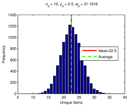
Fig. 4: Distribution of the number of unique edges on 10,000 random trials.

From equation (2), we can determine the number of extra edges needed in Phase 1. Specifically, we insert $w^{(1)}=\sum_{b}w_{b}$ edges to get a total of $m^{(1)}=\sum_{b}m_{b}$ unique Phase 1 edges. We let $w_{g}$ be the sum of the weights of all its constituent blocks. For generating a Phase 1 edge, the process for a single edge proceeds as follows:

1. Pick an affinity group randomly, where the probability of picking group $g$ is proportional to its weight $w_{g}$.

2. Pick a block within the affinity group uniformly at random (all blocks within the same group have the same weight).

3. Pick two nodes uniformly at random without replacement from the selected block — these two nodes form an edge.

The first step is a weighted sampling step and requires $O(\log g_{{\rm max}})$ work, where $g_{{\rm max}}\leq d_{{\rm max}}$ is the total number of affinity groups. The other 2 steps are constant time operations.

3.6 Phase 2

Phase 2 is simply applying the Chung-Lu model on the expected excess degrees. In creating an edge, we choose two nodes independently. Those nodes are chosen proportional to their excess degree. For node $i$ in group $b$, let $w_{i}=\frac{1}{2}[d_{i}-(\rho_{b}\cdot d_{b})]$ denote half its excess degree. The total number of edges that should be inserted in Phase 2 is $w^{(2)}=\sum_{i}w_{i}$. Ignoring duplicate edges (which are fairly rare in our experiments), we have $m^{(2)}=w^{(2)}$ Phase 2 edges.

Let $n^{\rm fill}_{d}$ and $n_{d}^{\rm bulk}$ be the number of filler and bulk nodes of degree $d$, let $w_{d}=\sum_{i\in V_{d}}w_{i}$ be the weight of all degree-$d$ nodes, and let $r_{d}$ be the proportion that are filler nodes. Inserting a Phase 2 edge proceeds as follows:

1. Pick degree $d$, where the probability of picking degree $d$ is proportional to $w_{d}$.

2. Pick between filler and bulk nodes by selecting a uniform random number $x\in[0,1]$ and choosing filler if $x<r_{d}$ and bulk otherwise.

3. Pick a filler or bulk node (as determined in Step 2) of degree $d$, uniformly at random.

The first step is a weighted sampling step and required $O(\log(d_{{\rm max}}))$ work, while the other two steps are constant time operations.

One complication in Phase 2 is that getting the correct number of degree-1 nodes poses a problem — approximately 36% of the pool of potential degree-1 nodes will not be selected and another 28% will have degree 2 or larger. A fix for this problem has been proposed in [15], which involves increasing the pool of degree-1 nodes, without changing the the expected number of edges that will be connected to these vertices. This increase in the pool size is controlled by the “blowup factor,” $\beta\geq 1$. This is included in the setup described in Algorithm 1 (Line 16).

3.7 Independent Edge Generation

Lastly, we pull everything together to explain the independent edge generation. We insert a total of $w=w^{(1)}+w^{(2)}$ edges, flipping a weighted coin for each edge to determine if it is Phase 1 or Phase 2. We expect to generate a total of $m=m^{(1)}+m^{(2)}$ edges.

Generating the edges is extremely inexpensive: $O(\log(d_{{\rm max}}))$ per edge. The expensive step is de-duplication where extra copies of repeated edges are removed. The same difficulty exists for the current Graph 500 (SKG) benchmark. Some may argue that duplicate edges are a useful feature since real data also has duplicates, but it is not clear that the duplication rates are similar to those observed in real data.

3.8 BTER Sampling Implementation

BTER edge generation is shown in Algorithm 2. The procedure Random_Sample does a weighted sampling according to a specified discrete distribution. For $p$ bins, the cost is $O(\log(p))$. For each edge, we randomly select between the phases using a weighted coin. A Phase 1 edge requires one sample from a discrete distribution of size $g_{{\rm max}}$ and three additional random values drawn uniformly from $[0,1]$. A Phase 2 edges requires two samples from a discrete distribution of size $d_{{\rm max}}$ and four additional random values drawn uniformly from $[0,1]$. Since $g_{{\rm max}}\leq d_{{\rm max}}$, an upper bound on the cost per edge is the cost of one discrete random sample on a distribution of size $d_{{\rm max}}$ plus four random values drawn uniformly from $[0,1]$.

In Algorithm 2, we generate each edge independently. It may also be possible to “bulk” the computations by first determining the total number of edges for each phase and perform the computation for each phase separately. Within each phase, the procedure itself can be easily vectorized to boost runtime performance, as in MATLAB.

Algorithm 2 BTER Sample

1:procedure bter_sample($\set{n_{d}},\set{i_{d}},\set{w_{d}},\set{r_{d}},\set{n^{\rm fill}_{d}},\set{w_{g}},\set{i_{g}},\set{b_{g}},\set{n_{g}}$)

2:    $w^{(1)}\leftarrow\sum_{g}w_{g}$, $w^{(2)}\leftarrow\sum w_{d}$, $w\leftarrow w^{(1)}+w^{(2)}$

3:    $E\leftarrow\emptyset$

4:    for $j=1,\dots,w$ do

5:         $r\sim U[0,1]$

6:         if $r<w^{(1)}/w$ then

7:             $E\leftarrow E\;\cup$ bter_sample_phase1($\set{w_{g}},\set{i_{g}},\set{b_{g}},\set{n_{g}}$)

8:         else

9:             $E\leftarrow E\;\cup$ bter_sample_phase2($\set{w_{d}},\set{r_{d}},\set{n_{d}},\set{n^{\rm fill}_{d}},\set{i_{d}}$)

10:         end if

11:    end for

12:    return $E$

13:

14:procedure bter_sample_phase1($\set{w_{g}},\set{i_{g}},\set{b_{g}},\set{n_{g}}$)

15:    $g\leftarrow$ random_sample($\set{w_{g}}$) $\triangleright$ Choose group

16:    $r_{1}\sim U[0,1]$, $\delta=i_{g}+\lfloor r_{1}\cdot b_{g}\rfloor\cdot n_{g}$ $\triangleright$ Choose block and compute its offset

17:    $r_{2}\sim U[0,1]$, $i\leftarrow\lfloor r_{2}\cdot n_{g}\rfloor+\delta$ $\triangleright$ Choose 1st node

18:    $r_{3}\sim U[0,1]$, $j\leftarrow\lfloor r_{3}\cdot(n_{g}-1)\rfloor+\delta$ $\triangleright$ Choose 2nd node

19:    if $j\geq i$ then

20:         $j\leftarrow j+1$

21:    end if

22:    return $(i,j)$

23:

24:procedure bter_sample_phase2($\set{w_{d}},\set{r_{d}},\set{n_{d}},\set{n^{\rm fill}_{d}},\set{i_{d}}$)

25:    $i\leftarrow$ bter_sample_phase2_node($\set{w_{d}},\set{r_{d}},\set{n_{d}},\set{n^{\rm fill}_{d}},\set{i_{d}}$)

26:    $j\leftarrow$ bter_sample_phase2_node($\set{w_{d}},\set{r_{d}},\set{n_{d}},\set{n^{\rm fill}_{d}},\set{i_{d}}$)

27:    return $(i,j)$

28:

29:procedure bter_sample_phase2_node($\set{w_{d}},\set{r_{d}},\set{n_{d}},\set{n^{\rm fill}_{d}},\set{i_{d}}$)

30:    $d\leftarrow$ random_sample($\set{w_{d}}$) $\triangleright$ Choose degree

31:    $r_{1}\sim U[0,1]$, $r_{2}\sim U[0,1]$

32:    if $r_{1}<r_{d}$ then

33:         $i\leftarrow\lfloor r_{2}\cdot n^{\rm fill}_{d}\rfloor+i_{d}$ $\triangleright$ Fill node

34:    else

35:         $i\leftarrow\lfloor r_{2}\cdot(n_{d}-n^{\rm fill}_{d})\rfloor+(i_{d}+n^{\rm fill}_{d}$) $\triangleright$ Bulk node

36:    end if

37:    return $i$

3.9 Edge Deduplication

Any method can be used for deduplication. In general, the simplest procedure is to hash the edges in such a way that $(i,j)$ and $(j,i)$ hash to the same key. Then it is easy enough to sort each bucket to remove duplicates. In a parallel environment, since we are hashing by edge and not vertex, there should not be load balancing problems. In fact, hashing by a single endpoint is not recommended because of the heavy-tailed nature of the graph.

3.10 Implementations

We have a reference implementation in MATLAB that is available at http://www.sandia.gov/~tgkolda/feastpack/. We have also implemented the method in Hadoop MapReduce and use this version in some of our experiments. Since the BTER algorithm generates edges independently, map tasks can perform all the work of creating edges and reduce tasks simply remove duplicate edges; hence, the implementation runs as a single MapReduce job. Each map task is given the desired degree and clustering coefficient, which is sufficient to compute affinity blocks and sampling probabilities. Each map task uses a different seed for random number generation used in creating edges. Map tasks are assigned a fixed number of edges to generate. The default is one million edges, so a graph of $w$ edges requires $w/10^{6}$ map tasks. There is no HDFS input file for the map tasks; instead, we wrote a subclass of org.apache.hadoop.mapreduce.InputFormat that causes a map task to generate a given number of records. For each edge, the map emits a key-value pair consisting of a hash value for the edge (based on the two endpoints) and the endpoints. Note that there is no assignment of specific nodes to specific map or reduce tasks. The reducer tasks collect edges with the same hash value and remove any duplicates before emitting the final list of all edges. We enable Hadoop compression between the map and reduce phases for faster performance.

4 Numerical Comparisons

We consider the performance of BTER on various real-world data sets, including presently the largest publicly-available graph modeled in the sense of matching degree distribution. We provide additional plots in the appendices; specifically, log-binned data as well as cumulative degree distributions.

4.1 Small data

In Figure 5, we present comparisons of BTER with the state-of-the-art in scalable generative models: SKG [8, 27] and Chung-Lu [1, 10, 11, 15] on two small data sets available from SNAP [50]. We use SKG because it is the current choice as the Graph 500 generator [48]. We omit details here but instead refer the reader to the references listed above for the details of the method and to [45, 43] for and in-depth analysis and discussion of problems with SKG. The Chung-Lu model has been described in §2.3. We treat all edges as undirected and remove any duplicate edges and loops. The graph ca-AstroPh is a collaboration network based on 124 months of data from the astrophysics section of the arXiv preprint server; it has 9,987 nodes and 25,973 edges. The graph soc-Epinions1 is a who-trusts-whom online social (review) network from the Epinions website with 75,879 nodes and 405,740 edges.

The parameters of SKG are from [27]. The input to Chung-Lu is the degree distribution of the real graph and a blowup factor of $\beta=10$ [15]. The inputs to BTER are the degree distribution and clustering coefficients per degree (computed exactly by counting all wedges and triangles) of the real graph and a blowup factor of $\beta=10$. Timings are not reported as they are negligible for all three methods.

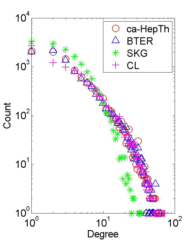
(a) Degree distribution for ca-HepTh

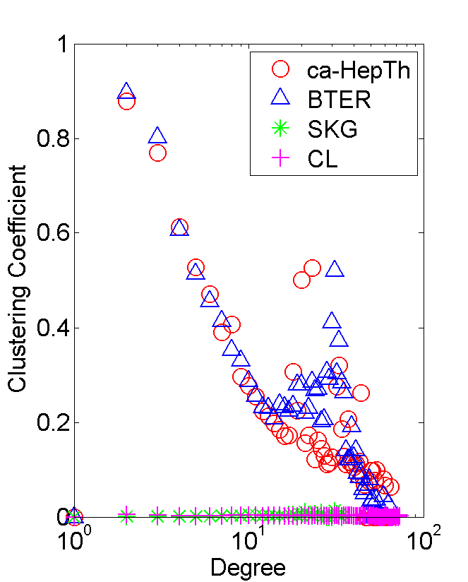
(b) Clustering coefficients for ca-HepTh

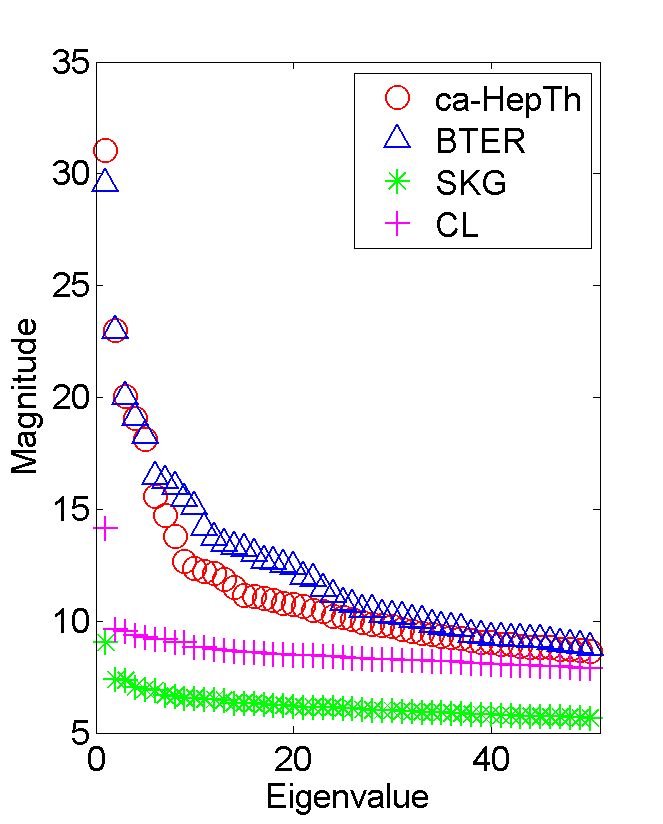
(c) Leading adjacency matrix eigenvalues for ca-HepTh

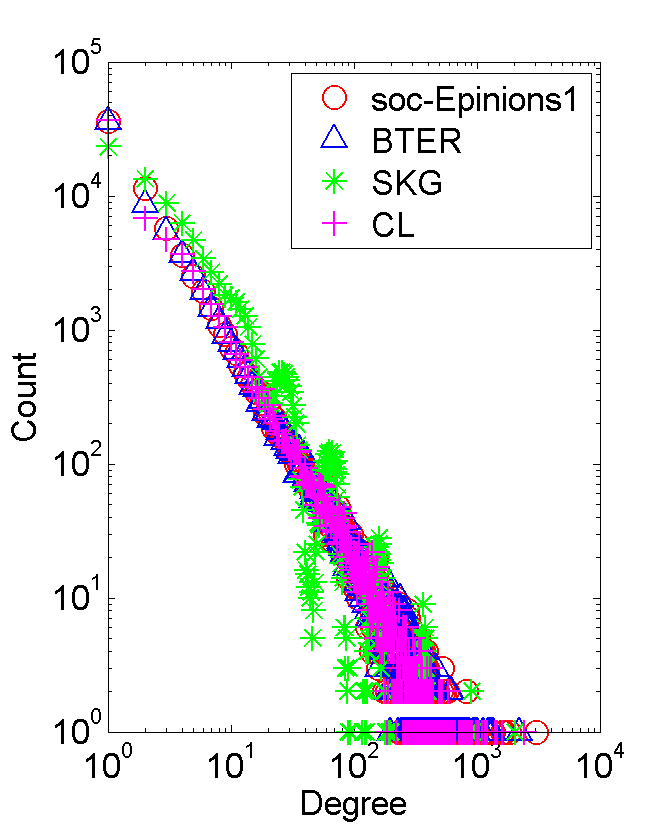
(d) Degree distribution for soc-Epinions1

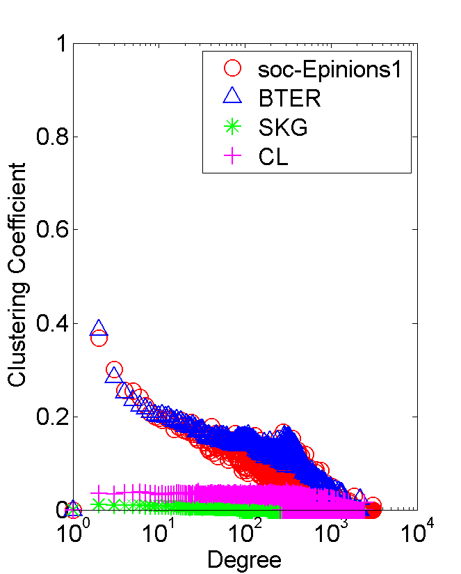
(e) Clustering coefficients for soc-Epinions1

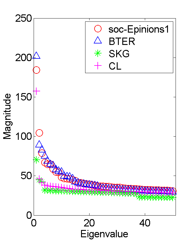
(f) Leading adjacency matrix eigenvalues for soc-Epinions1

Fig. 5: Comparison of Chung-Lu (CL), SKG, and BTER on small graphs.

Degree distribution

The degree distributions for the original graphs and the models are shown in Figures 5a and 5d. SKG is known to have oscillations in the degree distribution [45, 43], and these oscillations are easily visible in Figure 5d. The oscillations are correctable with appropriate addition of noise [45, 43] (not shown), but even then it tends to overestimate the low degree nodes and miss the highest degree nodes. In contrast, both Chung-Lu and BTER closely match the real data.

Clustering coefficients

The clustering coefficients per degree for the original graphs and the models are shown in Figures 5a and 5e. The SKG graph model has no inherent mechanism for closing triangles and creating a community structure. Though a few triangles may close at random, they are insufficient for the SKG-generated graph to match the clustering coefficients in the real data. The situation for Chung-Lu is similar to that for SKG — there is no reason for wedges to close. BTER, on the other hand, provides a much closer match to the real data.

Eigenvalues of adjacency matrix

We show the top 50 leading eigenvalues (in magnitude) of the adjacency matrix in Figures 5c and 5f. BTER provides a much closer match to the real data — especially the first few eigenvalues. Under certain circumstances, matching the degree distribution should produce a match in eigenvalues [29]. However, based on the observation that the eigenvalues of a graph with community structure are larger than those of the Chung-Lu graph with the same degree distribution, we conjecture that graphs with community structure require that triangle structure also be matched to obtain a good fit for the eigenvalues.

4.2 Large data

We demonstrate that BTER is able to fit large-scale real-world data. We do not compare to SKG because it is not possible to fit the parameters for such large graphs. We do not compare to the Chung-Lu model because we can easily explain the performance: its match in terms of the degree distribution is nearly identical to that of BTER, and its clustering coefficients are close to zero, for the small data. The data sets are described in Table 2a. We treat all edges as undirected and remove any duplicate edges and loops. We obtained real-world graphs from the Laboratory for Web Algorithms [49], which compressed the graphs using LLP and WebGraph [7, 5]. Briefly, the networks are described as follows.

• amazon-2008 [7, 5]: A graph describing similarity among books as reported by the Amazon store.

• ljournal-2008 [9, 7, 5]: Nodes represent users on LiveJournal. Node $x$ connects to node $y$ if $x$ registered $y$ as a friend.

• hollywood-2011 [7, 5]: This is a graph of actors. Two actors are joined by an edge whenever they appear in a movie together.

• twitter-2010 [26, 7, 5]: Nodes are Twitter users, and node $x$ links to node $y$ if $y$ follows $x$.

• uk-union-2006-06-2007-05 (shortened to uk-union) [6, 7, 5]: Links between web pages on the .uk domain. We ignore the time labeling on the links.

To the best of our knowledge, uk-union is the largest publicly available graph.

Table 2: Network characteristics of original and BTER-generated graphs.

Graph	$|V|$	$|E|$	$d_{{\rm max}}$	$d_{{\rm avg}}$	GCC
amazon-2008	1M	4M	1,077	10	0.260
ljournal-2008	5M	50M	19,432	18	0.124
hollywood-2011	2M	114M	13,107	115	0.175
twitter-2010	40M	1,202M	2,997,487	60	0.001
uk-union	122M	4,659M	6,366,528	76	0.007

(a) Large data set properties.

Graph	$|V|$	$|E|$	$d_{{\rm max}}$	$d_{{\rm avg}}$	GCC	Gen.	Dedup.
amazon-2008	1M	4M	1,052	10	0.253	2.27s	9.25s
ljournal-2008	5M	49M	18,510	19	0.127	33.81s	126.40s
hollywood-2011	2M	114M	11,676	115	0.180	88.54s	362.25s
twitter-2010	38M	1,135M	1,635,823	59	0.004	230s
uk-union	120M	4,405M	1,497,950	73	0.111	1350s

(b) Properties of BTER-generated graphs, including generation and edge deduplication time.

The smaller graphs (amazon-2008, ljournal-2008, hollywood-2011) are those with up to roughly 100M edges. These can be easily processed using MATLAB on an SGI Altix UV 10 with 32 cores (4 Xeon 8-core 2.0GHz processors) and 512 GB DDR3 memory. None of the parallel capabilities of MATLAB are enabled for these studies. To give a sense of the memory requirements, storing the hollywood-2011 graph as a sparse matrix in MATLAB requires 3.4GB of storage. The larger graphs (twitter-2010, uk-union) each have over 1B edges. These are processed on a Hadoop cluster with 32 compute nodes. Each compute node has an Intel i7 930 CPU at 2.8GHz (4 physical cores, HyperThreading enabled), 12 GB of memory, and 4 2TB SATA disks. All experiments were run using Apache Hadoop version 0.20.203.0. The results in Table 2b were obtained using 132 map and 32 reduce tasks.

The inputs to BTER are the degree distribution and clustering coefficients by degree. (We used a blowup of $\beta=1$ for the experiments reported here.) Computing the degree distribution is straightforward. However, for the clustering coefficients calculations, we used the sampling approach as implemented in [24] with 2000 samples per degree, so the expected error is $\epsilon=0.05$ at a confidence level of 99.9%. Sampling was not required for the smaller graphs, but we used it in all experiments for consistency.

BTER Timing

Table 2b shows the details and timings for the graphs produced by BTER. Observe the close match in the characteristics of the graphs in terms of number of nodes, number of edges, maximum degree, average degree, and global clustering coefficient. For the smaller graphs, we are able to separate the edge generation and deduplication time. The generation time is not strictly proportional to the number of desired edges because we have to generate extra edges for Phase 1 to account for possible duplicates (see §3.5). The parallelism of Hadoop yields a large advantage in terms of time. The twitter-2010 graph has 10 times more edges than hollywood-2011, but it takes less than half the time to do the computation on the 32-node Hadoop cluster.

Degree Distribution

Figure 6 illustrates the match between the real data and the BTER graph. BTER cannot easily match discontinuities in the degree distribution because of the randomness in creating edges. The issue is that nodes generally do not get exactly the desired degree; in the realization of the graph, observed degrees may deviate by one or two from the expected degree. For a smooth degree distribution, neighboring degrees cancel the effect of one on another. For discontinuous distributions, the BTER degree distribution is a “smoothed” version. This is evident, for instance, in the amazon-2008 data where we can see a smoothing effect on the sharp discontinuity near degree 10.

(a) amazon-2008

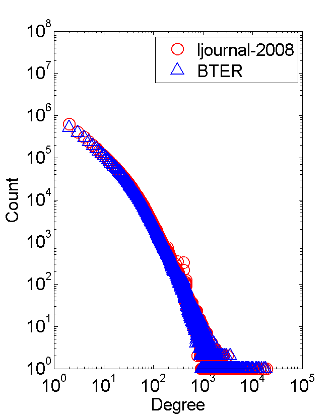
(b) ljournal-2008

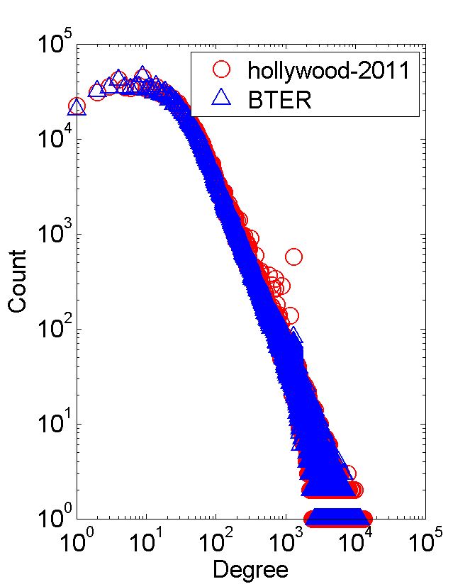
(c) hollywood-2011

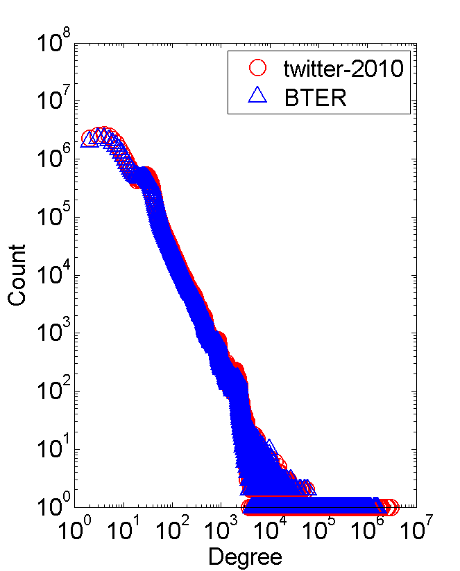
(d) twitter-2010

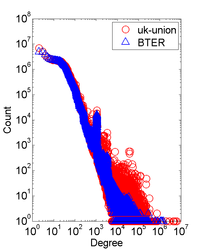
(e) uk-union

Fig. 6: Degree distributions of original and BTER-generated graphs.

Clustering Coefficients

BTER’s strength is its ability to match clustering coefficients and therefore create community structure. Most degree distributions are heavy-tailed and have a relatively consistent structure. The same is not true for clustering coefficients. Different profiles can potentially lead to graphs with fundamentally different structures. Figure 7 shows the clustering coefficients of the real data and the BTER-generated graphs. There is a very close match.

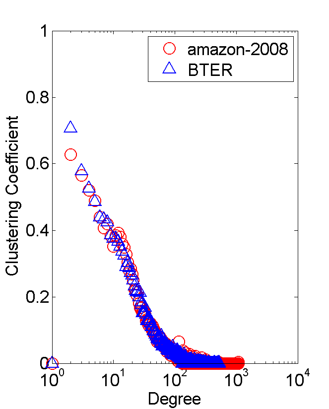
(a) amazon-2008

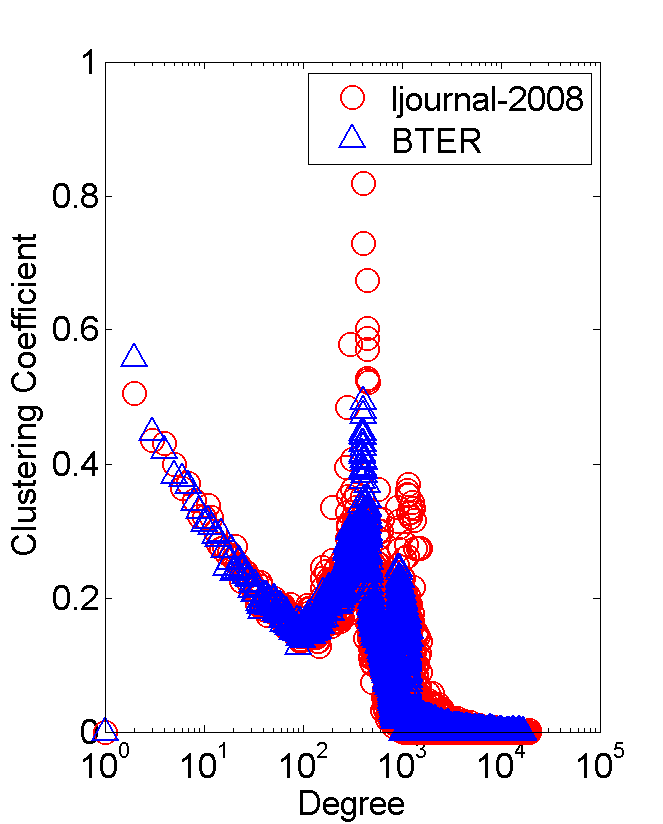
(b) ljournal-2008

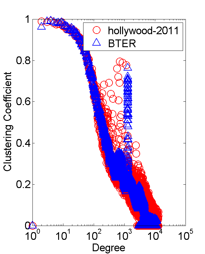
(c) hollywood-2011

(d) twitter-2010

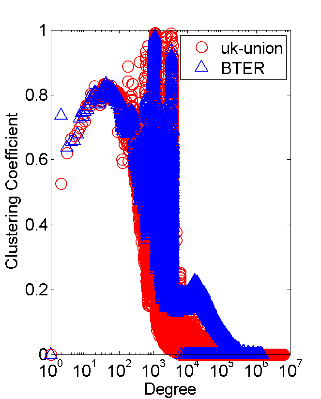
(e) uk-union

Fig. 7: Clustering coefficients of original and BTER-generated graphs.

5 Proposed Benchmark Parameters and Scalability

Thus far we have considered how BTER can be used to match real-world data. For benchmarking purposes, where there is no specific graph to be matched, “ideal” profiles for degree distribution and clustering coefficient by degree are required. In this section, we propose some possibilities, noting that these are tunable for various testing scenarios, i.e., specifying an average degree, a maximum clustering coefficient, etc. Generating an artificial degree distribution can be problematic. For instance, using a straight power law distribution can lead to impossible situations, like choosing a degree greater than the number of nodes. This necessitates a discrete distribution, which engenders its own problems. After proposing methods for working around these problems, we use the proposed benchmark in a scalability study for the MapReduce implementation of BTER.

5.1 Idealized Degree Distribution

It has been hypothesized that degree distribution of real-world networks follow a power law (PL) degree distribution, i.e.,

$$n_{d}\propto d^{-\gamma},$$

for some parameter $\gamma$ [2]. However, our observation is that power law distributions are difficult to use as a model — a point that is discussed in more detail below. It has been suggested that power laws are not necessarily the best descriptors for real-world networks [41, 4]. Finally, proving (in a statistical sense) that a single observed degree distribution is power law is difficult [13].

For benchmarking purposes, our goal is to specify an ideal average degree, $\bar{d}$, and an absolute bound on maximum degree, $d^{*}$. Let $f(d)$ define the desired proportionality of degree $d$, e.g., $f(d)=d^{-\gamma}$ for a power law distribution. We then create a discrete distribution on $d=1,\dots,d^{*}$ as

$$\text{Pr}\left(D=d\right)=\frac{f(d)}{\sum_{d^{\prime}=1}^{d^{*}}f(d^{\prime})}.$$

Ideally, the average degree is equal to $\bar{d}$ and the probability of having degree $d^{*}$ is sufficiently small, i.e.,

$$\bar{d}=\sum_{d=1}^{d^{*}}d\cdot f(d)\quad\text{and}\quad\text{Pr}\left(D=d^{*}\right)<\epsilon_{\rm tol},$$

where $\epsilon_{\rm tol}$ is small enough such that $n\cdot\epsilon_{\rm tol}\ll 1$ (where $n$ is the number of nodes). For the power law distribution, it can be difficult to find a value for $\gamma$ that yields a high enough average degree and a low enough probability of choosing $d^{*}$. Hence, we propose instead a generalized log-normal (GLN) distribution, i.e.,

$$n_{d}\propto\exp\left[-\left(\frac{\log d}{\alpha}\right)^{\delta}\right],$$

for some parameters $\alpha$ and $\delta$. The appendices includes example degree distributions that vary $\alpha$ and $\delta$. The shape of the distribution is typical of the real-world graphs shown in §4.

We consider two scenarios, both with $n=10^{7}$ nodes. We do a parameter search on $\alpha$ and $\delta$ (fminsearch in MATLAB) to locate the optimal parameters. A function degdist_param_search that finds the optimal parameters for either discrete GLN or discrete PL for user-specified values of $d_{{\rm avg}}$ and $d_{{\rm max}}$ is included in the reference code to be released at a future date.

Scenario 1 for Degree Distribution Fitting

In the first scenario, the targets are $\bar{d}=16$ and $d^{*}=10^{6}$. For discrete PL, the optimal parameter is $\gamma=1.911$ with $d_{{\rm avg}}=16$ and $\text{Pr}\left(D=d^{*}\right)=1.97\times 10^{-12}$. For discrete GLN, the optimal parameters are $\alpha=1.988$ and $\delta=2.079$ with $d_{{\rm avg}}=16$ and $\text{Pr}\left(D=d^{*}\right)=4.14\times 10^{-26}$. Realizations of the two distributions are pictured in Figure 8a. For this scenario, both degree distributions are reasonable in that there is no sharp dropoff as we get close to the maximum allowable degree, $d^{*}$.

Scenario 2 for Degree Distribution Fitting

In the second scenario, the targets are $\bar{d}=64$ and $d^{*}=10^{5}$. For PL, the optimal parameter is $\gamma=1.668$ with $d_{{\rm avg}}=64$ but $\text{Pr}\left(D=d^{*}\right)=2.16\times 10^{-9}$ (fairly large). For discrete GLN, the optimal parameters are $\alpha=2.171$ and $\delta=1.877$ with $d_{{\rm avg}}=64$ and $\text{Pr}\left(D=d^{*}\right)=8.35\times 10^{-12}$. Realizations of the two distributions are pictured in Figure 8b. In this scenario, the problem with power law becomes apparent — near $d^{*}$, there are still many degrees with multiple nodes so that the cutoff is extremely abrupt. In comparison, discrete GLN fades more naturally to the desired maximum degree.

(a) Scenario 1: $\bar{d}=16$ and $d^{*}=10^{6}$

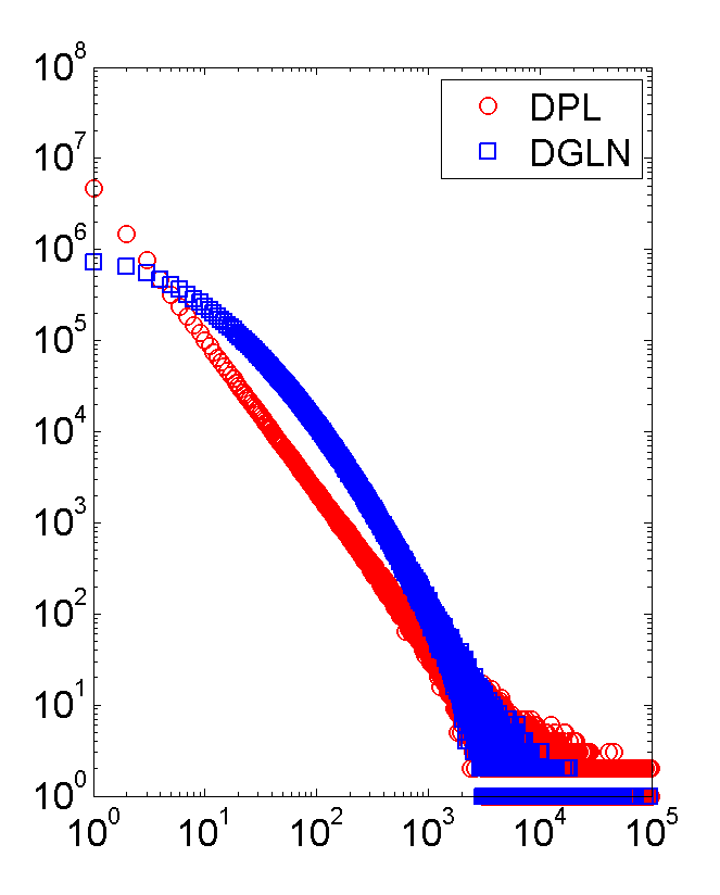
(b) Scenario 2: $\bar{d}=64$ and $d^{*}=10^{5}$

Fig. 8: Example degree distributions from discrete power law (DPL) and discrete generalized log normal (DGLN) for $n=10^{7}$ nodes.

5.2 Idealized Clustering Coefficients

As there is no definitive structure to clustering coefficients, we propose a simple parameterized curve that has some similarity to real data observations.

Let $\set{n_{d}}$ define the specified degree distribution and $d_{{\rm max}}$ be the maximum degree such that $n_{d}>0$. We define $\bar{c}_{d}$, the mean value for $c_{d}$, as

$$\bar{c}_{d}=c_{\rm max}\exp(-(d-1)\cdot{\xi})\quad\text{for}\quad d\geq 2,$$

where $c_{\rm max}$ and $\xi$ are parameters. If $c_{\rm max}$ is specified, then a simple parameter search can be used to fit $\xi$ to a target global clustering coefficient; code to fit the data is included in the reference code. The final values for $\set{c_{d}}$ are selected as

$$c_{d}\sim\mathcal{N}(\bar{c}_{d},\min\{10^{-2},\bar{c}_{d}/2\}).$$

The randomness could, of course, be omitted.

5.3 Example Graphs

We generate two example graphs per the scenarios below. Table 3 lists the network characteristics and Figure 9 shows the target and BTER-generated degree distributions and clustering coefficients.

Table 3: Network characteristics of BTER-generated graphs for benchmarking.

Graph	$|V|$	$|E|$	$d_{{\rm max}}$	$d_{{\rm avg}}$	GCC	Gen.	Dedup.
Scenario 1	1M	35M	28,643	72	0.406	35.11s	117.18s
Scenario 2	1M	8M	2,594	17	0.104	5.07s	20.66s

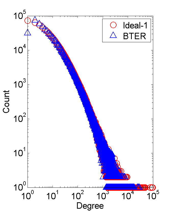
(a) Degree distribution for Scenario 1

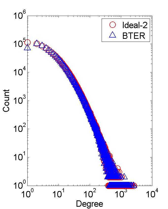
(b) Degree distribution for Scenario 2

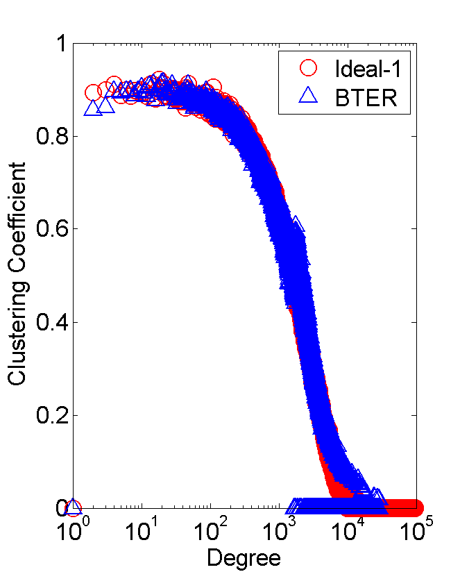
(c) Clustering coefficients for Scenario 1

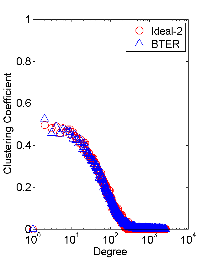
(d) Clustering coefficients for Scenario 2

Fig. 9: Target distributions and results of BTER-generated graphs.

Scenario 1

For the first set-up, we selected $\bar{d}=75$ and $d^{*}=100,000$ to define the degree distribution. The parameter search selected $\alpha=2.14$ and $\delta=1.83$. For the clustering coefficients, we set $c_{\rm max}=0.9$ and a target GCC of 0.15. The parameter search selected $\xi=3.59\times 10^{-4}$ for defining the clustering coefficient profile.

Scenario 2

For the second set-up, we selected $\bar{d}=16$ and $d^{*}=10,000$ to define the degree distribution. The parameter search selected $\alpha=1.98$ and $\delta=2.08$. For the clustering coefficients, we set $c_{\rm max}=0.5$ and a target GCC of 0.10. The parameter search selected $\xi=0.01$ for defining the clustering coefficient profile.

5.4 Scalability Test

We use the DGLN distribution to create target distributions that define a series of graphs of different sizes but similar community structure. From these, we generate example graphs with our Hadoop MapReduce implementation of BTER and demonstrate scalability of our code.

Table 4 describes characteristics of the test graphs. We selected $\bar{d}=32$ for all graphs and maintained $d^{*}$ proportional to $\sqrt{|V|}$, a relation that we often observe in social network graphs. The last two columns of the table list the number of generated (phase 1 and 2) and unique edges measured from full graphs realized by BTER.

Target degree distributions were created using the formulas and functions presented in §5.1. Optimal parameters $\alpha$ and $\delta$ were computed using MATLAB function degdist_param_search (part of the reference code). The function takes $\bar{d}$ and $d^{*}$ as inputs, plus the $\text{Pr}\left(D=d^{*}\right)$ which we set to $0.001/|V|$. Then we computed a discrete GLN from $\alpha$, $\delta$, and the number of nodes $|V|$ listed in the second column of Table 4. We created clustering coefficient distributions as in §5.2, setting $c_{\rm max}=0.5$ and $\mbox{GCC}=0.15$ for all graphs.

Table 4: Graph characteristics for testing BTER scalability.

Graph	$|V|$	$d^{*}$	$\bar{d}$	gen $|E|$	unique $|E|$
1	1M	50k	32	25M	16M
2	2M	70k	32	50M	32M
3	4M	100k	32	101M	64M
4	8M	140k	32	201M	128M
5	16M	200k	32	403M	256M
6	32M	280k	32	808M	512M
7	64M	400k	32	1,614M	1,024M
8	128M	570k	32	3,233M	2,047M
9	256M	800k	32	6,467M	4,096M

The MapReduce implementation of BTER was executed on a 32-node cluster running Apache Hadoop version 0.20.203.0. Each compute node contains a quad-core processor and four hard drives configured to run independently (no RAID striping). Hadoop was configured for a maximum of 128 simultaneous map tasks, effectively pairing each core with a hard drive for maximum I/O throughput. A MapReduce job can therefore launch up to 128 mappers in parallel. Hadoop was also configured for a maximum of 128 simultaneous reduce tasks. BTER uses the reduce phase to remove duplicate edges, so we expect this to compete for machine resources with BTER map tasks that generate phase 1 and phase 2 edges.

Figure 10a renders the data in Table 4, showing how the computational work varies across test graphs. To assess scalability in the weak sense, we set the workload of each map task in BTER to be 1 million edges; hence, Graph #1 executes with 1 map task and Graph #9 executes with 256. The number of reduce tasks was set to the number of map tasks, up to the configured Hadoop limit of 128.

Figure 10b plots BTER execution time (wall clock time) as a function of the number of vertices requested. Perfect scalability would appear as a horizontal line. We observe excellent scalability up to 32 million vertices (32 map tasks), and then a significant dropoff in parallel performance. However, map task scalability is excellent through 128 tasks, the full capacity of the cluster. Hence, BTER edge generation in the map phase is fully scalable to the available hardware. Removal of duplicate edges in the reduce phase is less scalable. Here the edges must be sorted on the map task node, shuffled across the network to reduce task nodes, and merged at the reducers. Close examination of Hadoop log files and network traffic suggest that the reduce phase suffers from bandwidth limitations during the shuffle and from spillover to disk during the merge. We conjecture that deduplication scalability could be improved on a cluster with larger network bandwidth and more physical memory per compute node.

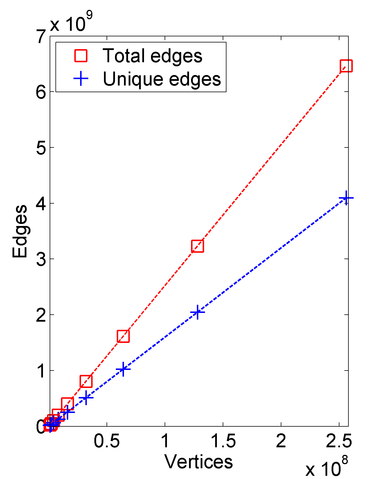
(a) Test graph sizes

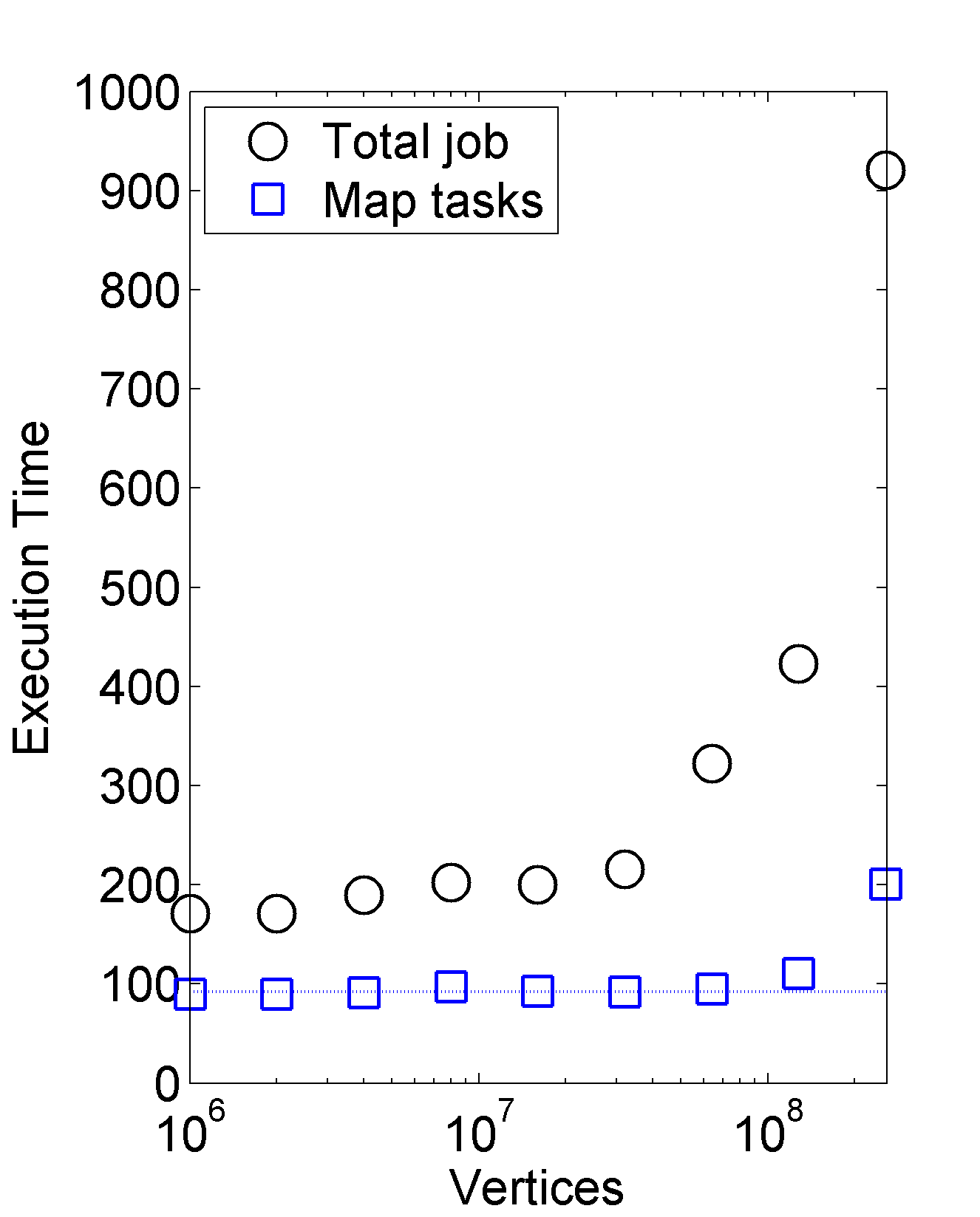
(b) BTER execution time in seconds

Fig. 10: Scalability of BTER MapReduce implementation.

We also show an example of the generated graph in Figure 11. This is for Graph #9 with 256M vertices and 4B edges. We give log-binned results. The BTER model is fairly close to the intended distributions for both the degree distribution and the clustering coefficient by degree.

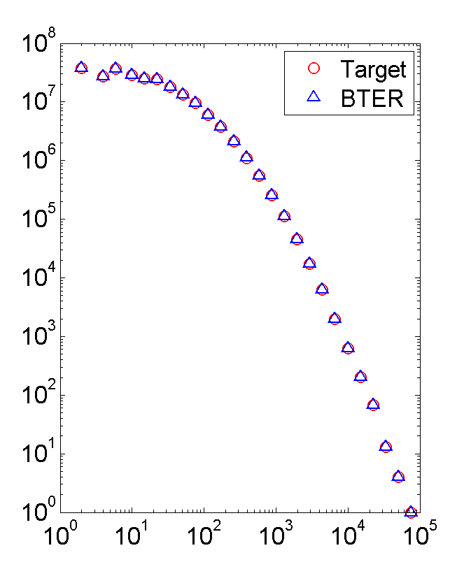
(a) Degree distribution (log-binned)

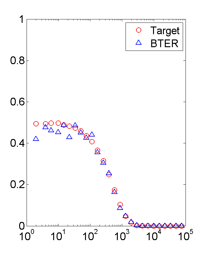
(b) Clustering coefficients (log-binned)

Fig. 11: Example target and actual degree distributions for 256M nodes using proposed idealized distributions.

6 Conclusions and Future Work

This paper demonstrates that the BTER generative model is useful for modeling massive networks, especially as compared with other scalable models. We provide a detailed algorithm along with analysis explaining the workings of the method. The original paper on BTER [42] provided none of the implementation details and, in fact, did not directly use the clustering coefficient data but rather estimated it via a function. Here we give precise details on the implementation, which is nontrivial due to issues such as repeat edges. We are able to build a model of a graph with 120M nodes and 4.4B edges in less than 25 minutes on a 32-node Hadoop cluster.

The development of a realistic graph model is an important step in developing effective “null” models that nonetheless share the properties of real-world networks. Such models will be useful in detecting anomalies, statistical sampling, and community detection. For example, the BTER model does not have larger communities beyond the affinity blocks, whereas we might expect that real-world graphs have a richer structure such as a hierarchy or other complex behavior.

The proposed BTER model, along with the proposed degree and clustering coefficient distributions, may also boost benchmarking efforts in graph processing. The proposed degree distributions capture the essence of degree distributions that we see in practice and generate realistic distributions even at large scales (whereas power law has a reputation of generating a few degrees that are much larger than observed in practice). Moreover, the proposed distribution allows us to modify both the average and the maximum degree, which is critical for benchmarking. The proposed clustering coefficient curves implicitly embed triangle structure into the graphs, which is a critical feature that distinguishes real graphs form arbitrary sparse graphs. And finally, the proposed generation algorithm scales to extremely large graphs because it generates edges in parallel.

Of course, we should list the limitations of the BTER model. First and foremost, we only consider simple graphs. More complex models would be needed for directed and/or weighted graphs. For instance, even capturing the degree distributions of a directed graph is a challenge [15]. We also ignore complex community structure, such as bipartite or near-bipartite community structure as well as hierarchical structure, which has been observed in real-world applications [38, 12]. Such structure could potentially be incorporated by adjusting the way that affinity blocks are linked. Currently, affinity blocks link only within themselves and then randomly to other nodes in the graphs. To simulate bipartite structure, the affinity blocks could be paired. To generate hierarchical structure, the affinity blocks could be arranged in that way with excess degree being biased towards blocks that are closer in the hierarchy. We do not incorporate node and edge types which would be relevant, for instance, in an e-commerce graph that represents users and items, connected via purchases and ratings of items by users. Finally, although we can generate edges in a streaming fashion, the BTER model has no real concept of evolving parameters in time. All of these issues are topics for future studies.

Appendix A Coupon Collector Derivation

Consider a universe $U$ of objects/coupons, and suppose we pick objects uniformly at random with replacement from $U$. The following theorem proves the bound used in equation (2), when $U$ is the set of possible pairs in an affinity block (so $|U|=\binom{n_{b}}{2}$). This is a simple take on the standard coupon collector problem, where we wish to pick up all distinct coupons. (We follow the analysis of Section 3.6.1 in [34]).

Theorem 1.

For a given $\rho\in(0,1)$, the expected number of independent draws required to select $\rho|U|$ distinct coupons from $U$ is $|U|\ln(1/(1-\rho))+O(1)$.

Proof.

For convenience, we assume that $\rho|U|$ is an integer. Consider a sequence of draws. Let $X_{i}$ (for integer $0\leq i<\rho|U|$) be the random variable denoting the number of draws required to get one more (distinct) coupon after $i$ distinct coupons have been collected. Observe that the quantity of interest is $\mathbb{E}[\sum_{i<\rho|U|}X_{i}]$, which by linearity of expectation is $\sum_{i<\rho|U|}\mathbb{E}[X_{i}]$. (The usual coupon collector analyses consider this sum for $\rho=1$.)

When $i$ distinct coupons have already been collected, the probability that a single draw gives a new coupon is exactly $1-i/|U|$. Think of this as probability of “failure.” The number of draws required for a success (new coupon) follows a geometric distribution (Chap VI.8 of [17]) and the mean of this is $1/(1-i/|U|)=|U|/(|U|-i)$. Using this bound, the expected total number of draws can be expressed as follows:

$$\sum_{i<\rho|U|}\mathbb{E}[X_{i}] =\sum_{i<\rho|U|}\frac{|U|}{|U|-i}$$

$$=|U|\Big{[}\sum_{i\leq|U|}\frac{1}{i}-\sum_{i\leq(1-\rho)|U|}\frac{1}{i}\Big{]}$$

$$=|U|\Big{[}\ln|U|-\ln((1-\rho)|U|)+O(1/|U|)\Big{]}=|U|\ln(1/(1-\rho))+O(1)$$

(We use the standard bound for the Harmonic sum: $\sum_{i\leq r}1/i=\ln r+\gamma+O(1/r)$, where $\gamma$ is Euler-Mascheroni constant.) ∎

Appendix B Plots with Log-Binned Data

Figures 12 – 15 reproduce degree distribution and clustering coefficient plots in the original paper using logarithmic binning of the degrees. The $k$th degree bin covers the range $\set{b_{k},\dots,b_{k+1}-1}$ where

$$b_{k}=\left\lceil\frac{\omega^{k-1}-1}{\omega-1}\right\rceil+1.$$

We use $\omega=1.5$, which mean that the bin grows in size by 50% at each step. For example, the first few $b_{k}$ values are

$$\set{1,2,4,6,10,15,22,34,51,76,115,172,259,389,583,875,1313,1970,2955,\dots}$$

For the degree distributions, the data within each bin is summed. For the clustering coefficients by degree, the data within each bin is averaged.

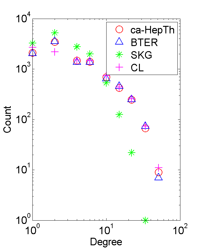
(a) Degree distribution for ca-HepTh

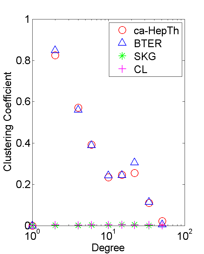
(b) Clustering coefficients for ca-HepTh

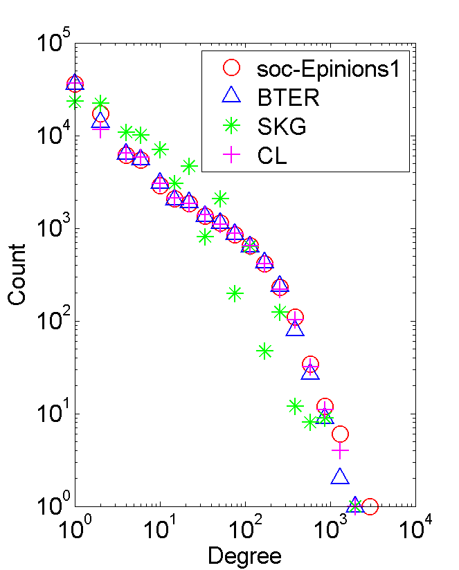
(c) Degree distribution for soc-Epinions1

(d) Clustering coefficients for soc-Epinions1

Fig. 12: Comparison of Chung-Lu (CL), SKG, and BTER on small graphs. (Reproduces Figure 5 in the original paper with log-binned plots.)

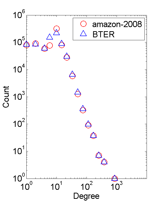
(a) amazon-2008

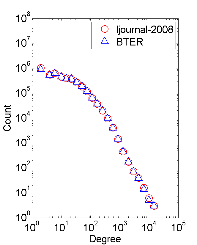
(b) ljournal-2008

(c) hollywood-2011

(d) twitter-2010

(e) uk-union

Fig. 13: Degree distributions of original and BTER-generated graphs. (Reproduces Figure 6 in the original paper with log-binned plots.)

(a) amazon-2008

(b) ljournal-2008

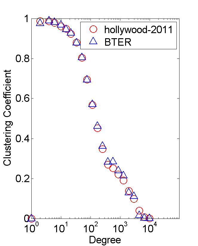
(c) hollywood-2011

(d) twitter-2010

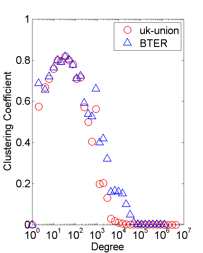
(e) uk-union

Fig. 14: Clustering coefficients of original and BTER-generated graphs. (Reproduces Figure 7 in the original paper with log-binned plots.)

(a) Degree distribution for Scenario 1

(b) Degree distribution for Scenario 2

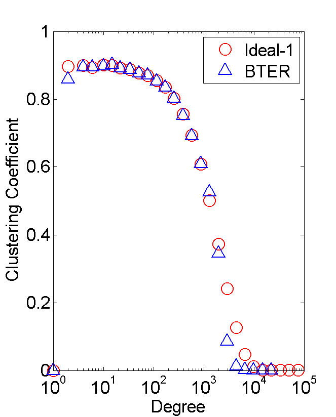
(c) Clustering coefficients for Scenario 1

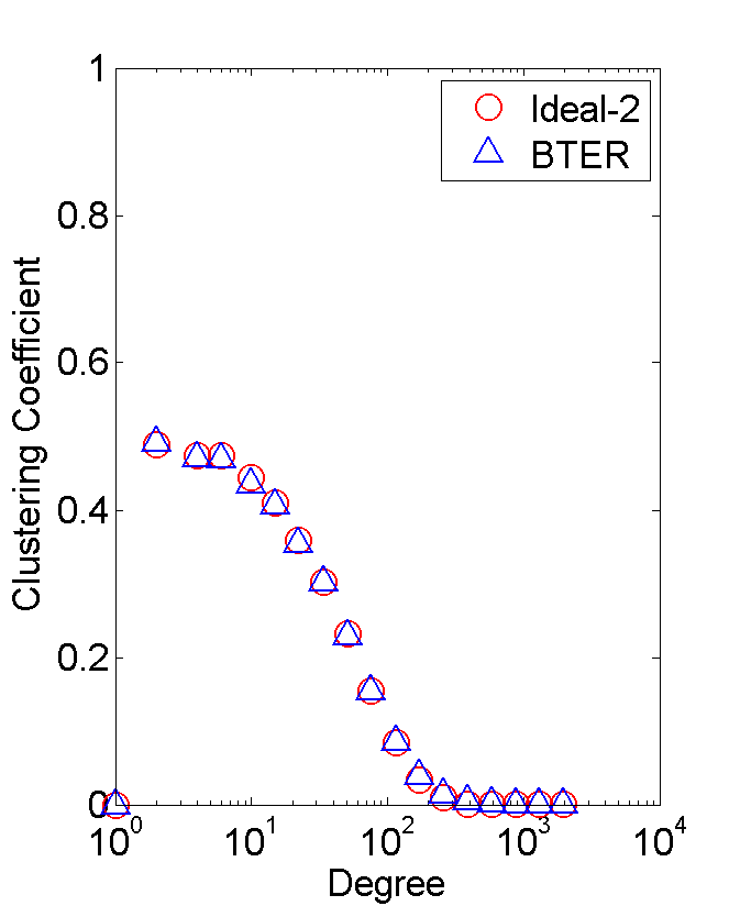
(d) Clustering coefficients for Scenario 2

Fig. 15: Target distributions and results of BTER-generated graphs. (Reproduces Figure 9 in the original paper with log-binned plots.)

Appendix C Cumulative Degree Distributions

Figures 16 – 18 reproduce degree distribution plots in the original paper using cumulative data.

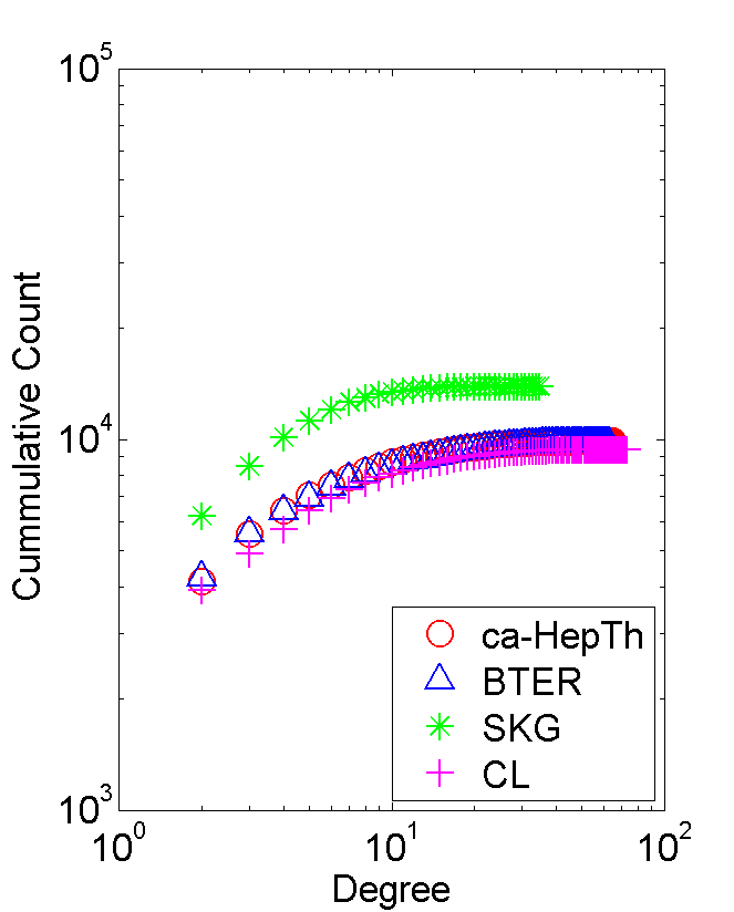
(a) Degree distribution for ca-HepTh

(b) Degree distribution for soc-Epinions1

Fig. 16: Comparison of Chung-Lu (CL), SKG, and BTER on small graphs. (Reproduces Figure 5 in the original paper with cumulative plots.)

(a) amazon-2008

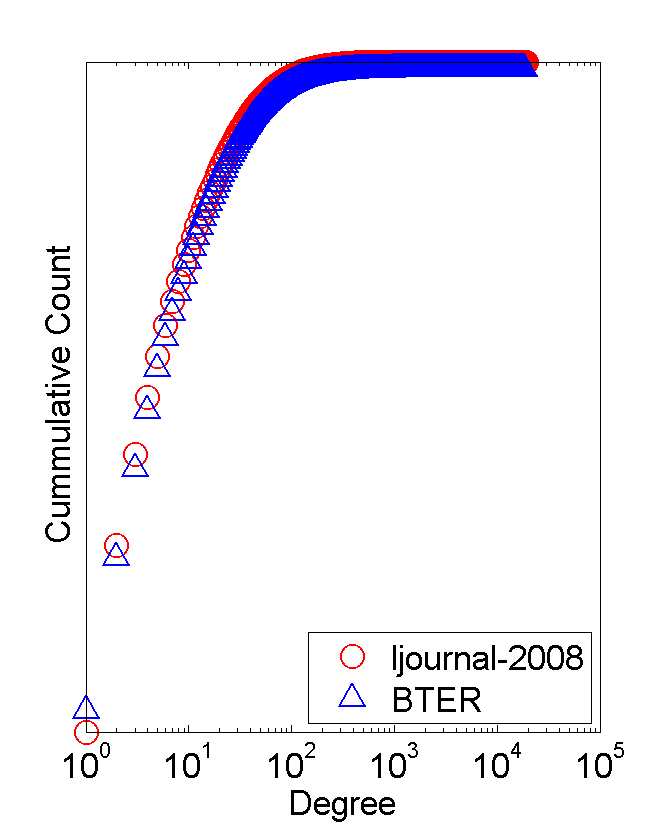
(b) ljournal-2008

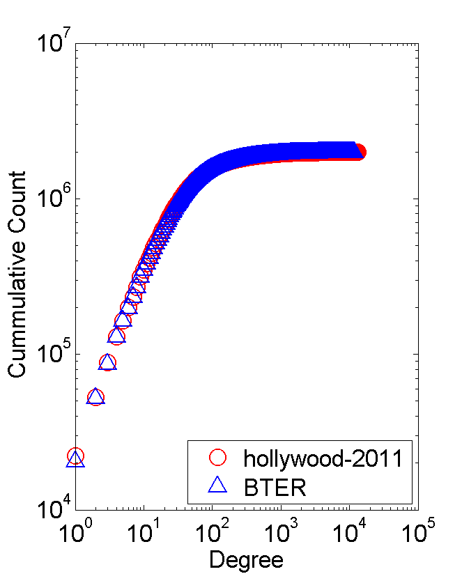
(c) hollywood-2011

(d) twitter-2010

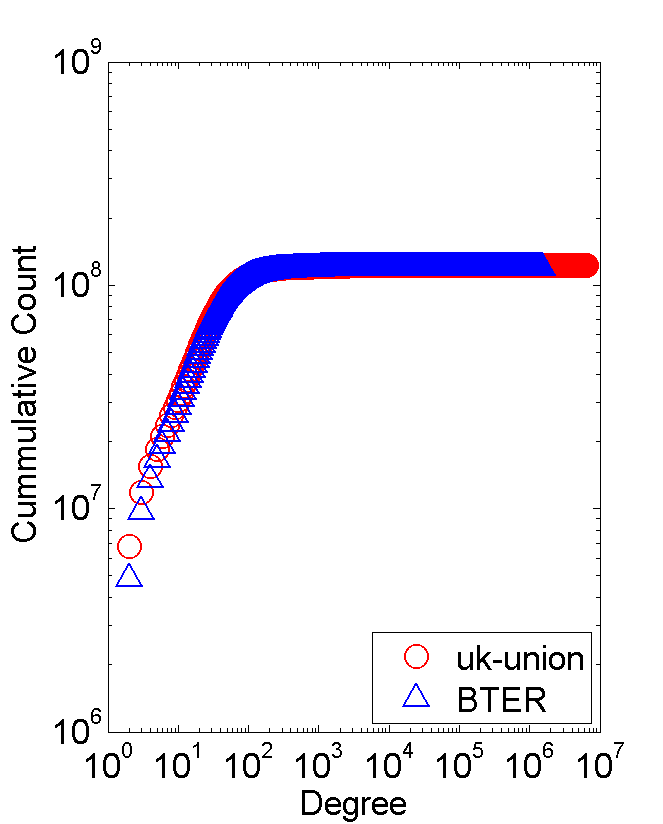
(e) uk-union

Fig. 17: Cumulative degree distributions of original and BTER-generated graphs. (Reproduces Figure 6 in the original paper with cumulative plots.)

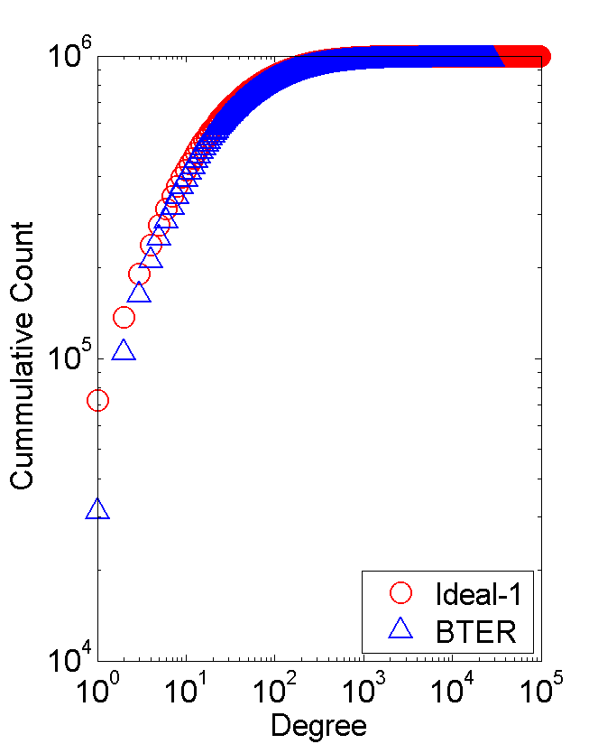
(a) Degree distribution for Scenario 1

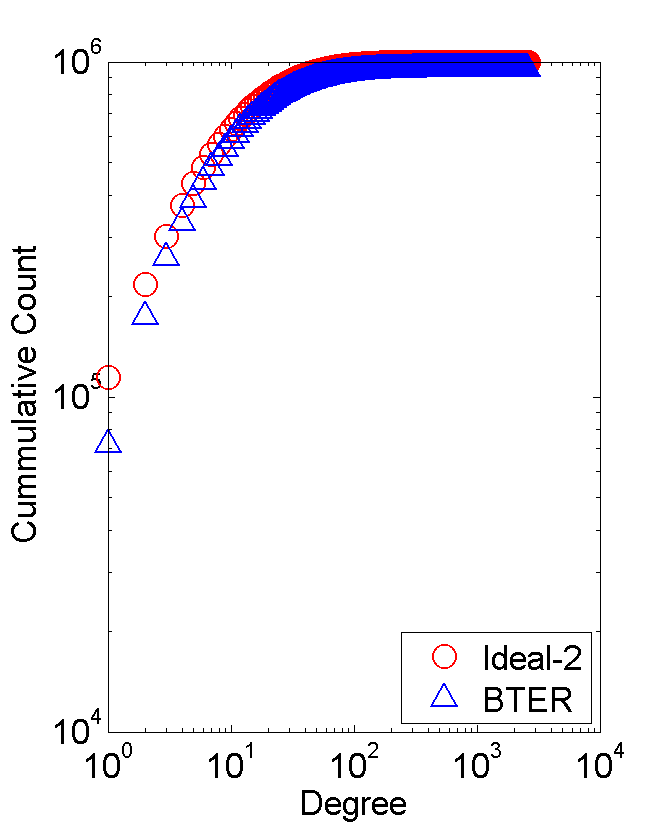
(b) Degree distribution for Scenario 2

Fig. 18: Cumulative target distributions and results of BTER-generated graphs. (Reproduces Figure 9 in the original paper with cumulative plots.)

Appendix D Parameter Study for Generalized Log-Normal Distribution

In Figure 19, we generate some example degree distributions using different parameters for the DGLN distribution, described in §5.1 or the paper. Here we use a maximum degree of $d^{*}=10^{6}$ and the number of nodes is $n=10^{7}$.

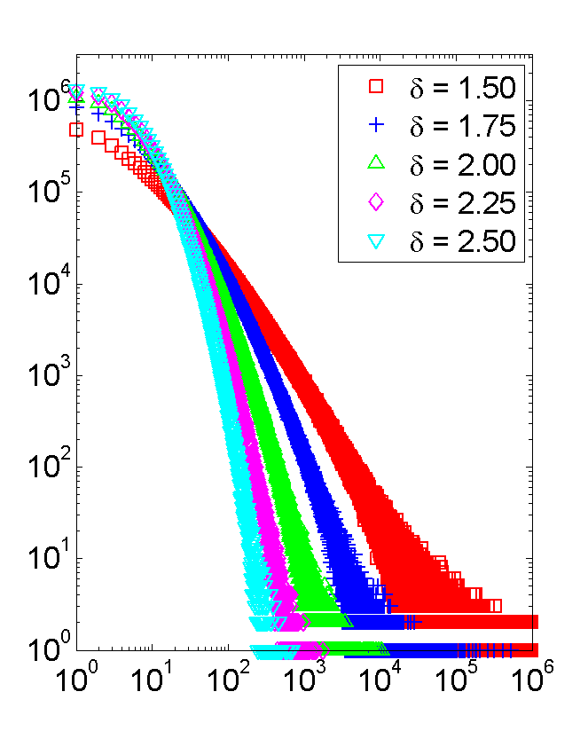
(a) $\alpha=2$ and $\delta$ varies

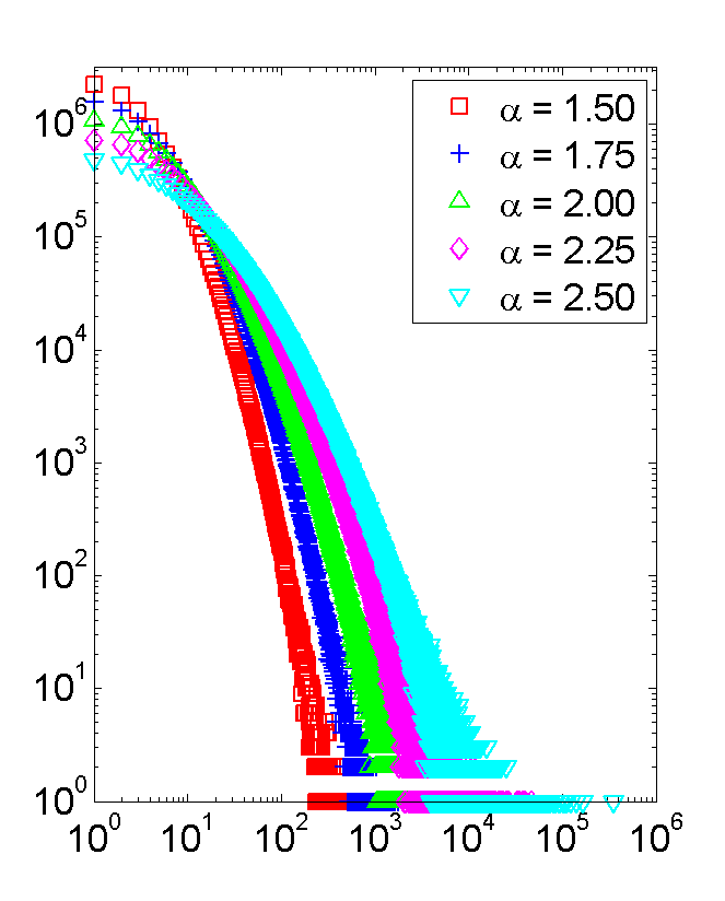
(b) $\alpha$ varies and $\delta=2$

Fig. 19: Sample degree distributions using different parameters for DGLN.

References

- [1] W. Aiello, F. Chung, and L. Lu, A random graph model for power law graphs, Experimental Mathematics, 10 (2001), pp. 53–66.
- [2] A.-L. Barabási and R. Albert, Emergence of scaling in random networks, Science, 286 (1999), pp. 509–512.
- [3] A. Barrat and M. Weigt, On the properties of small-world network models, The European Physical Journal B - Condensed Matter and Complex Systems, 13 (2000), pp. 547–560.
- [4] Z. Bi, C. Faloutsos, and F. Korn, The “DGX” distribution for mining massive, skewed data, in KDD ’01: Proceedings of the seventh ACM SIGKDD international conference on Knowledge discovery and data mining, ACM, 2001, pp. 17–26.
- [5] P. Boldi, M. Rosa, M. Santini, and S. Vigna, Layered label propagation: A multiresolution coordinate-free ordering for compressing social networks, in WWW’11: Proceedings of the 20th international conference on World Wide Web, ACM Press, 2011.
- [6] P. Boldi, M. Santini, and S. Vigna, A large time-aware graph, SIGIR Forum, 42 (2008), pp. 33–38.
- [7] P. Boldi and S. Vigna, The webgraph framework I: Compression techniques, in WWW’04: Proceedings of the 13th International Conference on World Wide Web, ACM Press, 2004, pp. 595–602.
- [8] D. Chakrabarti, Y. Zhan, and C. Faloutsos, R-MAT: A recursive model for graph mining, in SDM04: Proceedings of the Fourth SIAM International Conference on Data Mining, April 2004.
- [9] F. Chierichetti, R. Kumar, S. Lattanzi, M. Mitzenmacher, A. Panconesi, and P. Raghavan, On compressing social networks, in KDD ’09: Proceedings of the 15th ACM SIGKDD international conference on Knowledge discovery and data mining, ACM, 2009, pp. 219–228.
- [10] F. Chung and L. Lu, The average distances in random graphs with given expected degrees, Proceedings of the National Academy of Sciences, 99 (2002), pp. 15879–15882.
- [11] F. Chung and L. Lu, Connected components in random graphs with given degree sequences, Annals of Combinatorics, 6 (2002), pp. 125–145.
- [12] A. Clauset, C. Moore, and M. Newman, Hierarchical structure and the prediction of missing links in networks, Nature, 453 (2008).
- [13] A. Clauset, C. R. Shalizi, and M. E. J. Newman, Power-law distributions in empirical data, SIAM Review, 51 (2009), pp. 661–703.
- [14] D. Dominguez-Sal, P. Urbón-Bayes, A. Giménez-Vanó, S. Gómez-Villamor, N. Mart nez-Bazán, and J. Larriba-Pey, Survey of graph database performance on the HPC scalable graph analysis benchmark, in Web-Age Information Management, H. Shen, J. Pei, M. Özsu, L. Zou, J. Lu, T.-W. Ling, G. Yu, Y. Zhuang, and J. Shao, eds., vol. 6185 of Lecture Notes in Computer Science, Springer Berlin / Heidelberg, 2010, pp. 37–48.
- [15] N. Durak, T. G. Kolda, A. Pinar, and C. Seshadhri, A scalable directed graph model with reciprocal edges, in Proceedings of the IEEE 2nd Workshop on Network Science, 2013. to appear, also available as arXiv:1210.5288.
- [16] P. Erdös and A. Rényi, On the evolution of random graphs, Publication of the Mathematical Institute of the Hungarian Academy Of Sciences, (1960).
- [17] W. Feller, An Introduction to probability theory and applications: Vol I, John Wiley and Sons, 3rd ed., 1968.
- [18] M. Girvan and M. E. J. Newman, Community structure in social and biological networks, Proceedings of the National Academy of Sciences, 99 (2002), pp. 7821–7826.
- [19] D. F. Gleich and A. B. Owen, Moment-based estimation of stochastic Kronecker graph parameters, Internet Mathematics, 8 (2012), pp. 232–256.
- [20] W. Guo and S. Kraines, A random network generator with finely tunable clustering coefficient for small-world social networks, in CASON ’09: International Conference on Computational Aspects of Social Networks, June 2009, pp. 10–17.
- [21] R. Gupta, T. Roughgarden, and C. Seshadhri, Decompositions of triangle-dense graphs. arXiv:1309.7440, Sept. 2013.
- [22] A. Gutfraind, L. A. Meyers, and I. Safro, Multiscale network generation. arXiv:1207.4266, July 2012.
- [23] J. Kepner, The Kronecker theory of power law graphs, in Graph Algorithms in the Language of Linear Algebra, J. Kepner and J. Gilbert, eds., SIAM, 2011.
- [24] T. G. Kolda, A. Pinar, T. Plantenga, C. Seshadhri, and C. Task, Counting triangles in massive graphs with MapReduce. arXiv:1301.5887, Jan. 2013.
- [25] R. Kumar, P. Raghavan, S. Rajagopalan, D. Sivakumar, A. Tomkins, and E. Upfal, Stochastic models for the web graph, in Proceedings of 41st Annual Symposiumon Foundations of Computer Science, 2000, pp. 57–65.
- [26] H. Kwak, C. Lee, H. Park, and S. Moon, What is Twitter, a social network or a news media?, in WWW ’10: Proceedings of the 19th international conference on World wide web, New York, NY, USA, 2010, ACM, pp. 591–600.
- [27] J. Leskovec, D. Chakrabarti, J. Kleinberg, C. Faloutsos, and Z. Ghahramani, Kronecker graphs: An approach to modeling networks, Journal of Machine Learning Research, 11 (2010), pp. 985–1042.
- [28] J. Leskovec, J. Kleinberg, and C. Faloutsos, Graph evolution: Densification and shrinking diameters, ACM Transactions on Knowledge Discovery from Data, 1 (2007). Article No. 2.
- [29] M. Mihail and C. Papadimitriou, On the eigenvalue power law, in RANDOM 2002: Proceedings of Randomization and Approximation Techniques in Computer Science, vol. 2483 of Lecture Notes in Computer Science, Springer Berlin / Heidelberg, 2002, pp. 254–262.
- [30] B. Miller, N. Bliss, and P. Wolfe, Subgraph detection using eigenvector L1 norms, in NIPS 2010: Advances in Neural Information Processing Systems 23, 2010, pp. 1633–1641.
- [31] B. Miller, L. Stephens, and N. Bliss, Goodness-of-fit statistics for anomaly detection in Chung-Lu random graphs, in ICASSP 2012: IEEE International Conference on Acoustics, Speech and Signal Processing, march 2012, pp. 3265–3268.
- [32] D. Mir and R. N. Wright, A differentially private estimator for the stochastic Kronecker graph model, in EDBT-ICDT ’12: Proceedings of the 2012 Joint EDBT/ICDT Workshops, ACM, 2012, pp. 167–176.
- [33] S. Moreno, S. Kirshner, J. Neville, and S. V. N. Vishwanathan, Tied Kronecker product graph models to capture variance in network populations, in Proceedings of 2010 48th Annual Allerton Conference on Communication, Control, and Computing, Oct. 2010, pp. 1137–1144.
- [34] R. Motwani and P. Raghavan, Randomized Algorithms, Cambridge University Press, 1995.
- [35] M. Newman, Component sizes in networks with arbitrary degree distributions, Physical Review E, 76 (2007).
- [36] M. Newman, D. Watts, and S. Strogatz, Random graph models of social networks, Proceedings of the National Academy of Sciences, 99 (2002), pp. 2566–2572.
- [37] M. E. J. Newman, Properties of highly clustered networks, Phys. Rev. E, 68 (2003), p. 026121.
- [38] M. E. J. Newman, Finding community structure in networks using the eigenvectors of matrices, Physical Review E, 74 (2006), p. 036104.
- [39] A. Pinar, C. Seshadhri, and T. G. Kolda, The similarity between stochastic Kronecker and Chung-Lu graph models, in SDM12: Proceedings of the Twelfth SIAM International Conference on Data Mining, Apr. 2012, pp. 1071–1082.
- [40] A. Sala, L. Cao, C. Wilson, R. Zablit, H. Zheng, and B. Y. Zhao, Measurement-calibrated graph models for social network experiments, in WWW ’10: Proceedings of the 19th international conference on World wide web, 2010, pp. 861–870.
- [41] A. Sala, S. Gaito, G. P. Rossi, H. Zheng, and B. Y. Zhao, Revisiting degree distribution models for social graph analysis. arXiv:1108.0027, July 2011.
- [42] C. Seshadhri, T. G. Kolda, and A. Pinar, Community structure and scale-free collections of Erdös-Rényi graphs, Physical Review E, 85 (2012), p. 056109.
- [43] C. Seshadhri, A. Pinar, and T. G. Kolda, An in-depth study of stochastic Kronecker graphs, in ICDM 2011: Proceedings of the 2011 IEEE International Conference on Data Mining, 2011, pp. 587–596.
- [44] , Triadic measures on graphs: The power of wedge sampling. arXiv:1202.5230 [cs.SI], October 2012. to appear in SDM13.
- [45] , An in-depth analysis of stochastic Kronecker graphs, Journal of the Association for Computing Machinery, in press (2013). Preprint: http://arxiv.org/abs/1102.5046.
- [46] J. C. Vivar and D. Banks, Models for networks: a cross-disciplinary science, Wiley Interdisciplinary Reviews: Computational Statistics, 4 (2012), pp. 13–27.
- [47] D. Watts and S. Strogatz, Collective dynamics of ‘small-world’ networks, Nature, 393 (1998), pp. 440–442.
- [48] Graph 500 benchmark. Available at http://www.graph500.org/Specifications.html.
- [49] LWA: Laboratory for Web Algorithms. Available at http://law.di.unimi.it/datasets.php.
- [50] SNAP: Stanford Network Analysis Project. Available at http://snap.stanford.edu/.