Analytic form of the effective potential in the large $N$ limit of a real scalar theory in four dimensions

Abstract

We give the large $N$ limit of the effective potential for the $O(N)$ linear sigma model in four dimensions in terms of the Lambert $W$ function. The effective potential is fully consistent with the renormalization group, and it admits an asymptotic expansion in powers of a small positive coupling parameter. Careful consideration of the UV cutoff present in the model validates the physics of the large $N$ limit.

I Introduction

The physics of the $O(N)$ linear sigma model in four dimensions is well known. The model has two phases: the symmetric phase where the $N$ scalar fields obtain the same mass, and the broken phase where the spontaneous breaking of $O(N)$ to $O(N-1)$ gives rise to $N-1$ massless Nambu-Goldstone bosons. In the large $N$ limit, the model becomes weakly coupled and can be studied in details:Coleman:1974jh ; Coleman:1985 ; Moshe:2003xn ; Coleman:1985 the physical meaning of the triviality can be elucidated, and the physical equivalence between the linear and non-linear versions of the model, for a large enough UV cutoff, can be demonstrated explicitly. For three dimensions, an analytic form of the large $N$ limit of the effective potential has been known for a long time (see, for example, Coleman:1974jh ; David:1985zz ), and the existence of the non-trivial Wilson-Fisher fixed point has also been shown explicitly. In four dimensions, however, such an analytic form of the effective potential has not been given to the author’s knowledge.

It is the purpose of this short paper to give an exact analytic form of the effective potential in the large $N$ limit of the $O(N)$ linear sigma model in four dimensions. The obtained effective potential is not only fully consistent with the renormalization group (RG), but it also illuminates the nature of asymptotic expansions in powers of a small coupling. Since we assume the smallness of the physical mass compared with the UV cutoff, our effective potential is valid only for the VEV of a scalar field much smaller than the cutoff.

At the end of the paper, we have added a section to defend the physics of the large $N$ limit. We resolve the two problems raised in Coleman:1974jh by taking into account the presence of a UV cutoff.

II The large $N$ limit of the $O(N)$ linear sigma model

We consider the $O(N)$ linear sigma model in four dimensional Euclidean space. The effective potential for the large $N$ limit has been determined implicitly in Coleman:1974jh . We extend the result to give an explicit analytic form of the effective potential using the Lambert $W$ function.wiki:LambertW

The action is given by

$$S[\phi]=\int d^{4}x\,\left[\frac{1}{2}\left(\partial_{\mu}\phi^{I}\partial_{\mu}\phi^{I}\right)+\frac{m_{0}^{2}}{2}\left(\phi^{I}\phi^{I}\right)+\frac{\lambda_{0}}{8N}\left(\phi^{I}\phi^{I}\right)^{2}\right]$$ (1)

where the repeated $I$ is summed over $I=1,\cdots,N$. We introduce a constant source $j$ and define a generating function $w(j)$ by

$$\hbox{e}^{-Nw(j)\int d^{4}x}=\int\left[d\phi^{I}\right]\,\exp\left[-S[\phi]+\sqrt{N}j\int d^{4}x\,\phi^{N}(x)\right]$$ (2)

so that

$$-w^{\prime}(j)=v\equiv\frac{1}{\sqrt{N}}\left\langle\phi^{N}\right\rangle$$ (3)

We then define the effective potential by the Legendre transform

$$V_{\mathrm{eff}}(v)\equiv w(j)+vj$$ (4)

To compute $V_{\mathrm{eff}}$, we invert (3) to give $j$ in terms of $v$. We then integrate

$$V_{\mathrm{eff}}^{\prime}(v)=j$$ (5)

to obtain $V_{\mathrm{eff}}$.

The method of the large $N$ limit is well known.Coleman:1974jh ; Coleman:1985 ; Moshe:2003xn We first introduce an auxiliary field $\alpha(x)$ to rewrite the action with source as

$$S[\phi,\alpha] = \int d^{4}x\Bigg{[}\frac{1}{2}\left(\partial_{\mu}\phi^{I}\partial_{\mu}\phi^{I}\right)+\frac{m_{0}^{2}}{2}\left(\phi^{I}\phi^{I}\right)+\frac{\lambda_{0}}{8N}\left(\phi^{I}\phi^{I}\right)^{2}$$ (6)

$$\quad+\frac{N}{2\lambda_{0}}\left(\alpha+i\frac{\lambda_{0}}{2N}\left(\phi^{I}\phi^{I}\right)\right)^{2}-\sqrt{N}j\phi^{N}\Bigg{]}$$

$$= \int d^{4}x\left[\frac{1}{2}\left(\partial_{\mu}\phi^{I}\partial_{\mu}\phi^{I}\right)+\frac{1}{2}\left(m_{0}^{2}+i\alpha\right)\left(\phi^{I}\phi^{I}\right)+\frac{N}{2\lambda_{0}}\alpha^{2}-\sqrt{N}j\phi^{N}\right]$$

In the large $N$ limit, let $\Delta m_{0}^{2}$ be the saddle point value of $i\alpha$, which is determined by

$$\frac{1}{2}\left(v^{2}+\int\frac{d^{4}p}{(2\pi)^{4}}\frac{1}{p^{2}+m_{0}^{2}+\Delta m_{0}^{2}}\right)=\frac{\Delta m_{0}^{2}}{\lambda_{0}}$$ (7)

$\left\langle\phi^{N}\right\rangle=\sqrt{N}v$ gives

$$v\left(m_{0}^{2}+\Delta m_{0}^{2}\right)=j=V_{\mathrm{eff}}^{\prime}(v)$$ (8)

Eqs. (7) and (8) are Eqs. (2.7) and (2.8) of Ref. Coleman:1974jh . In the following we first solve (7) to determine $m_{0}^{2}+\Delta m_{0}^{2}$ in terms of $v$. It is then straightforward to obtain $V_{\mathrm{eff}}(v)$ by integrating (8).

To begin with, we introduce

$$m^{2}_{\mathrm{ph}}\equiv m_{0}^{2}+\Delta m_{0}^{2}$$ (9)

which is the physical squared mass of the field $\phi^{I}$. We assume that it is non-negative, and that it is extremely small compared with the square of the UV cutoff $\Lambda_{0}$:

$$0\leq m^{2}_{\mathrm{ph}}\ll\Lambda_{0}^{2}$$ (10)

We then obtain

$$\int\frac{d^{4}p}{(2\pi)^{4}}\frac{1}{p^{2}+m^{2}_{\mathrm{ph}}}=A_{4}\Lambda_{0}^{2}+\frac{m^{2}_{\mathrm{ph}}}{(4\pi)^{2}}\left\{\ln\frac{m^{2}_{\mathrm{ph}}}{\Lambda_{0}^{2}}+B_{4}\right\}+\mathrm{O}\left(\left(m^{2}_{\mathrm{ph}}\right)^{2}/\Lambda_{0}^{2}\right)$$ (11)

where $A_{4}$ and $B_{4}$ are regularization dependent constants. The assumption (10) allows us to ignore the corrections inversely proportional to $\Lambda_{0}^{2}$. Thus, (7) gives

$$m_{0}^{2} = m^{2}_{\mathrm{ph}}-\Delta m_{0}^{2}$$ (12)

$$= -\frac{\lambda_{0}}{2}A_{4}\Lambda_{0}^{2}+\frac{\lambda_{0}}{(4\pi)^{2}}\left[m^{2}_{\mathrm{ph}}\left(\frac{(4\pi)^{2}}{\lambda_{0}}-\frac{1}{2}\ln\frac{m^{2}_{\mathrm{ph}}}{\Lambda_{0}^{2}}-\frac{1}{2}B_{4}\right)-(4\pi)^{2}\frac{v^{2}}{2}\right]$$

Let us now introduce a renormalized coupling $\lambda$ by

$$\frac{\lambda}{(4\pi)^{2}}\equiv\frac{1}{\ln\frac{\Lambda_{0}}{\mu}+\frac{(4\pi)^{2}}{\lambda_{0}}-\frac{1}{2}B_{4}}$$ (13)

where $\mu$ is an arbitrary finite renormalization scale. It satisfies the RG equation

$$-\mu\frac{\partial}{\partial\mu}\frac{\lambda}{(4\pi)^{2}}=-\left(\frac{\lambda}{(4\pi)^{2}}\right)^{2}$$ (14)

We then introduce an RG invariant mass scale by

$$\Lambda\equiv\hbox{e}^{\frac{(4\pi)^{2}}{\lambda}}\mu$$ (15)

If $\frac{\lambda_{0}}{(4\pi)^{2}}$ is of order $1$, $\Lambda$ is of the same order as $\Lambda_{0}$.

Let us next introduce a squared mass parameter $m^{2}$ which is either positive or negative:

$$m_{0}^{2}=-\frac{\lambda_{0}}{2}A_{4}\Lambda_{0}^{2}+\frac{\lambda_{0}}{\lambda}m^{2}$$ (16)

The first term on the right is the critical squared mass; the $O(N)$ symmetry is exact for $m^{2}>0$, and spontaneously broken to $O(N-1)$ for $m^{2}<0$. The squared mass satisfies

$$-\mu\frac{\partial}{\partial\mu}m^{2}=-\frac{\lambda}{(4\pi)^{2}}m^{2}$$ (17)

Using (16), we can rewrite (12) as

$$m^{2}_{\mathrm{ph}}\left(1-\frac{\lambda}{(4\pi)^{2}}\frac{1}{2}\ln\frac{m^{2}_{\mathrm{ph}}}{\mu^{2}}\right)=m^{2}+\frac{1}{2}\lambda v^{2}$$ (18)

This is the same as (2.11) of Ref. Coleman:1974jh . With (15), this can be rewritten further as

$$\frac{m^{2}_{\mathrm{ph}}}{\Lambda^{2}}\ln\frac{m^{2}_{\mathrm{ph}}}{\Lambda^{2}}=\xi$$ (19)

where $\xi$ is short for the RG invariant

$$\xi\equiv-2\frac{\frac{(4\pi)^{2}}{\lambda}\left(m^{2}+\frac{1}{2}\lambda v^{2}\right)}{\Lambda^{2}}=\frac{m^{2}+\frac{1}{2}\lambda v^{2}}{\Lambda^{2}}\ln\frac{\mu^{2}}{\Lambda^{2}}$$ (20)

Since $m^{2}_{\mathrm{ph}}\ll\Lambda^{2}\simeq\Lambda_{0}^{2}$ by the assumption (10), we find

$$-\xi\ll 1$$ (21)

This corresponds to

$$v^{2}\ll\Lambda^{2}$$ (22)

Now, the solution of (19) is obtained by the lower branch of the Lambert $W$ function (or the product logarithm):

$$\ln\frac{m^{2}_{\mathrm{ph}}}{\Lambda^{2}}=W_{-1}(\xi)$$ (23)

where the negative valued $W_{-1}(\xi)$ is defined implicitly by

$$W_{-1}(\xi)\,\hbox{e}^{W_{-1}(\xi)}=\xi$$ (24)

for $\xi\in[-\frac{1}{\hbox{e}},0)$. (See Appendix for a little more details on $W_{-1}$.)

Using (8) and (9), we thus obtain

$$V_{\mathrm{eff}}^{\prime}(v) = vm^{2}_{\mathrm{ph}}=v\Lambda^{2}\exp\left[W_{-1}(\xi)\right]=v\Lambda^{2}\frac{\xi}{W_{-1}(\xi)}$$ (25)

$$= v\frac{-2\frac{(4\pi)^{2}}{\lambda}\left(m^{2}+\frac{1}{2}\lambda v^{2}\right)}{W_{-1}\left(\frac{-2\frac{(4\pi)^{2}}{\lambda}\left(m^{2}+\frac{1}{2}\lambda v^{2}\right)}{\Lambda^{2}}\right)}$$

We sketch the above for the two cases $m^{2}>0$ and $m^{2}<0$ in Fig. 1.

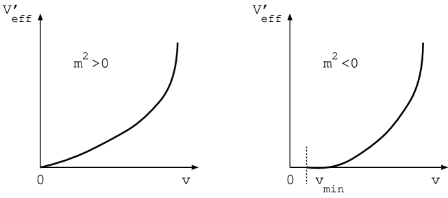
Figure 1: For $m^{2}>0$, $V_{\mathrm{eff}}$ is defined for $0\leq v\leq\sqrt{\frac{1}{(4\pi)^{2}}\Lambda^{2}\hbox{e}^{-1}-\frac{2m^{2}}{\lambda}}$. For $m^{2}<0$, it is defined for $v_{\mathrm{min}}\equiv\sqrt{\frac{-2m^{2}}{\lambda}}<v<\sqrt{\frac{1}{(4\pi)^{2}}\Lambda^{2}\hbox{e}^{-1}-\frac{2m^{2}}{\lambda}}$. At $v=v_{\mathrm{min}}$, $V_{\mathrm{eff}}^{\prime}=0$.

Obviously, the effective potential is minimized at $v=0$ for $m^{2}>0$, and at $v=v_{\mathrm{min}}\equiv\sqrt{\frac{-2m^{2}}{\lambda}}$ for $m^{2}<0$. The effective potential is valid only for $v^{2}\ll\Lambda^{2}$, and its behavior for $v\approx\Lambda$ should not be taken at a face value.

Integrating (25) with respect to $v$, we obtain the main result of this paper

$$V_{\mathrm{eff}}(v) = \frac{\Lambda^{4}}{(4\pi)^{2}}\frac{1}{8}\xi^{2}\left(\frac{1}{-\frac{1}{2}W_{-1}(\xi)}-\frac{1}{4}\frac{1}{\left(-\frac{1}{2}W_{-1}(\xi)\right)^{2}}\right)$$ (26)

$$= \frac{1}{(4\pi)^{2}}\frac{1}{2}\left\{\frac{(4\pi)^{2}}{\lambda}\left(m^{2}+\frac{1}{2}\lambda v^{2}\right)\right\}^{2}\left(\frac{1}{-\frac{1}{2}W_{-1}(\xi)}-\frac{1}{4}\frac{1}{\left(-\frac{1}{2}W_{-1}(\xi)\right)^{2}}\right)$$

where $\xi$ is given by (20). Here, we have arbitrarily chosen the integration constant so that $V_{\mathrm{eff}}$ vanishes at $\xi=0$. We note that our result is valid only for $-\xi\ll 1$.

To understand the structure of the effective potential, we introduce a physical coupling, defined for $m^{2}>0$, by

$$\frac{\lambda_{\mathrm{ph}}}{(4\pi)^{2}}\equiv\frac{1}{-\frac{1}{2}W_{-1}\left(\frac{m^{2}}{\Lambda^{2}}\ln\frac{\mu^{2}}{\Lambda^{2}}\right)}$$ (27)

which is an RG invariant. Especially for $m^{2}=\mu^{2}$, we find

$$\frac{\lambda_{\mathrm{ph}}}{(4\pi)^{2}}=\frac{\lambda}{(4\pi)^{2}}$$ (28)

Looking at the effective potential, we notice that $\frac{1}{-\frac{1}{2}W_{-1}(\xi)}$ is $\frac{\lambda_{\mathrm{ph}}}{(4\pi)^{2}}$, where the positive $m^{2}+\frac{\lambda}{2}v^{2}$ replaces $m^{2}$, not necessarily positive. Since the physical coupling admits an asymptotic expansion in powers of $\lambda>0$, the effective potential also admits such an asymptotic expansion.

At the minimum of $V_{\mathrm{eff}}$, we find

$$\frac{d^{2}V_{\mathrm{eff}}}{dv^{2}}\Big{|}_{\mathrm{minimum}}=\left\{\begin{array}[]{l@{\quad}l}m^{2}_{\mathrm{ph}}\Big{|}_{v=0}=m^{2}\frac{\lambda_{\mathrm{ph}}}{\lambda}&(m^{2}>0)\\ m^{2}_{\mathrm{ph}}\Big{|}_{\xi=0}=0&(m^{2}<0)\end{array}\right.$$ (29)

For $m^{2}>0$, this gives the physical squared mass of $\phi^{I}$ in the absence of a constant source. The vanishing for $m^{2}<0$ does not imply that $\phi^{N}$ is massless; only $\phi^{I}\,(I=1,\cdots,N-1)$ are massless, and $\phi^{N}$ which is coupled with the auxiliary field $\alpha$ has a squared mass of order $(-2m^{2})$. For $m^{2}>0$, the fourth order derivative of the effective potential at $v=0$ is not quite $\lambda_{\mathrm{ph}}$, but given by

$$\frac{1}{3}\frac{d^{4}}{dv^{4}}V_{\mathrm{eff}}(v=0)=\frac{\lambda_{\mathrm{ph}}}{1-\frac{1}{2}\frac{\lambda_{\mathrm{ph}}}{(4\pi)^{2}}}$$ (30)

For $m^{2}>0$, the two physical parameters $\frac{\lambda_{\mathrm{ph}}}{(4\pi)^{2}}$ and $m^{2}_{\mathrm{ph}}$ determine the effective potential uniquely.

III Defending the large $N$ limit

In Coleman:1974jh , two problems were found with the physics of the large $N$ limit. One is that the effective potential $V_{\mathrm{eff}}(v)$ is not well defined for $v$ of order $\Lambda$ and larger. The other is the presence of a tachyon pole in the propagator of $\phi^{N}$ in the broken phase. Both problems arise due to the neglect of the physical presence of an UV cutoff. We resolve them both in the following.

III.1 $V_{\mathrm{eff}}$ for large $v$

We have solved (19) to obtain the effective action. Its right-hand side is monotonically decreasing with $v^{2}$, but its left-hand side is monotonically decreasing with $m^{2}_{\mathrm{ph}}$ only for $m^{2}_{\mathrm{ph}}<\hbox{e}^{-1}\Lambda^{2}$. Thus, the one-to-one relationship between $v^{2}$ and $m^{2}_{\mathrm{ph}}$ is obtained only for $m^{2}_{\mathrm{ph}}<\hbox{e}^{-1}\Lambda^{2}$. Because of this, $V_{\mathrm{eff}}$ is defined only up to $v^{2}$ of order $\Lambda^{2}$. We find nothing wrong with this, since (19) is valid only for $v^{2}\ll\Lambda^{2}$.

In order to define $V_{\mathrm{eff}}$ for large $v$, we must introduce non-universality by keeping the neglected terms in the integral (11). Using a sharp momentum cutoff, we evaluate

$$\int\frac{d^{4}p}{(2\pi)^{4}}\frac{1}{p^{2}+m^{2}_{\mathrm{ph}}}\theta(\Lambda_{0}^{2}-p^{2})=\frac{1}{(4\pi)^{2}}\left[\Lambda_{0}^{2}+m^{2}_{\mathrm{ph}}\ln\frac{m^{2}_{\mathrm{ph}}}{\Lambda_{0}^{2}}-m^{2}_{\mathrm{ph}}\ln\left(1+\frac{m^{2}_{\mathrm{ph}}}{\Lambda_{0}^{2}}\right)\right]$$ (31)

corresponding to $A_{4}=\frac{1}{(4\pi)^{2}}$ and $B_{4}=0$. We keep the last term, which is non-universal.

The kept term changes (19) to

$$\frac{m^{2}_{\mathrm{ph}}}{\Lambda^{2}}\left[\ln\frac{m^{2}_{\mathrm{ph}}}{\Lambda^{2}}-\ln\left(1+\frac{m^{2}_{\mathrm{ph}}}{\Lambda^{2}}\hbox{e}^{2\frac{(4\pi)^{2}}{\lambda_{0}}}\right)\right]=\xi$$ (32)

where $\xi$ is defined by (20). As long as $\lambda_{0}>0$, the left-hand side is a monotonically decreasing function of $m^{2}_{\mathrm{ph}}\geq 0$. (See Fig. 2.)

Figure 2: We plot the left-hand side of (32) as a function of $x\equiv\frac{m^{2}_{\mathrm{ph}}}{\Lambda^{2}}$ for $\hbox{e}^{2\frac{(4\pi)^{2}}{\lambda_{0}}}=2$. It is monotonically decreasing as opposed to the approximation $x\ln x$ used for (19).

For $m^{2}_{\mathrm{ph}}\gg\Lambda^{2}$, we obtain

$$-2\frac{(4\pi)^{2}}{\lambda_{0}}m^{2}_{\mathrm{ph}}-\Lambda_{0}^{2}\simeq-2\frac{(4\pi)^{2}}{\lambda}\left(m^{2}+\frac{\lambda}{2}v^{2}\right)$$ (33)

where we have used

$$\Lambda_{0}^{2}=\Lambda^{2}\hbox{e}^{-2\frac{(4\pi)^{2}}{\lambda_{0}}}$$ (34)

This gives

$$V_{\mathrm{eff}}(v)\simeq m_{0}^{2}\frac{v^{2}}{2}+\frac{\lambda_{0}}{2}\left(\frac{v^{2}}{2}\right)^{2}$$ (35)

Thus, somewhat as expected, the effective potential for very large $v$ is given by the potential in the bare action.

III.2 Absence of tachyons in the broken phase

In the broken phase $m^{2}<0$ of the large $N$ limit, the propagator of $\phi^{N}$ is given by

$$\left\langle\phi^{N}(k)\phi^{N}(-k)\right\rangle=\frac{\frac{1}{\lambda_{0}}+\frac{1}{2}f\left(\frac{k^{2}}{\Lambda_{0}^{2}}\right)}{k^{2}\left(\frac{1}{\lambda_{0}}+\frac{1}{2}f\left(\frac{k^{2}}{\Lambda_{0}^{2}}\right)\right)+\frac{-2m^{2}}{\lambda}}$$ (36)

where we use a sharp cutoff to define

$$f\left(\frac{k^{2}}{\Lambda_{0}^{2}}\right)\equiv\int\frac{d^{4}p}{(2\pi)^{4}}\frac{1}{p^{2}(p+k)^{2}}\theta(\Lambda_{0}^{2}-p^{2})\theta(\Lambda_{0}^{2}-(p+k)^{2})$$ (37)

The above propagator is the same as (3.14) of Coleman:1974jh .

Note that

1. $f$ is non-negative, and is decreasing with $\frac{k^{2}}{\Lambda_{0}^{2}}$;

2. $f=0$ for $k^{2}\geq 4\Lambda_{0}^{2}$ due to the sharp UV cutoff.

Since the denominator of the propagator is strictly positive, there is no tachyonic pole.

We find a tachyonic pole, however, if we use an approximation of $f$. For $k^{2}\ll\Lambda_{0}^{2}$, we can approximate $f$ as follows:

$$f\left(\frac{k^{2}}{\Lambda_{0}^{2}}\right)\simeq\frac{1}{(4\pi)^{2}}\left(\ln\frac{\Lambda_{0}^{2}}{k^{2}}+1\right)$$ (38)

If we use this approximate expression, we find a tachyonic pole at

$$k^{2}\simeq\hbox{e}^{2\frac{(4\pi)^{2}}{\lambda_{0}}+1}\Lambda_{0}^{2}$$ (39)

But the approximation of $f$ is invalid for $k^{2}$ as large as this, and the pole is indeed absent as we have concluded above by a simple observation.

IV Conclusion

In conclusion, we have obtained the effective potential for the large $N$ limit of the $O(N)$ linear sigma model explicitly in terms of the Lambert $W$ function.

Our use of the Lambert $W$ function is by no means the first application in quantum field theory. It has been used to solve exactly the 2- and 3-loop RG equations in QCD.Gardi:1998qr ; Magradze:1998ng ; Magradze:1999um (See also Nesterenko:2003xb for a review of other applications in QCD.) It has also been applied for the study of general RG flows in Curtright:2010hq , and most recently by the author to solve generic 2-loop RG equations in theories with a Gaussian IR fixed point.Sonoda:2013b

*

Appendix A Lambert $W$ function

The Lambert $W$ function (a.k.a. product logarithm)wiki:LambertW is defined implicitly by

$$W(x)\hbox{e}^{W(x)}=x$$ (40)

Restricted to real values, the function has two branches: the upper $W_{0}(x)>-1$ defined for $x\in[-\hbox{e}^{-1},+\infty)$ and the lower $W_{-1}(x)<-1$ for $x\in[-\hbox{e}^{-1},0)$. (See Fig. 3.)

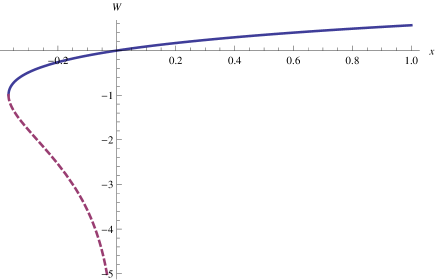
Figure 3: The real valued Lambert $W$ function has two branches: the upper $W_{0}$ (solid) and lower $W_{-1}$ (dashed).

For $-x\ll 1$, we obtain the asymptotic expansion

$$W_{-1}(x)=\ln(-x)-\ln\left(-\ln(-x)\right)+\mathrm{O}\left(\frac{\ln\left(-\ln(-x)\right)}{\ln(-x)}\right)$$ (41)

Perhaps the best known use of the Lambert $W$ function is for the distribution function

$$f(x)=\frac{x^{n}}{\hbox{e}^{x}-1}\quad(x>0)$$ (42)

with $n>0$. For $x>0$, it is maximized at $x=n+W_{0}(-n\hbox{e}^{-n})$.