Quadrature for second-order triangles in the Boundary Element Method

Abstract

A quadrature method for second-order, curved triangular elements in the Boundary Element Method (BEM) is presented, based on a polar coordinate transformation, combined with elementary geometric operations. The numerical performance of the method is presented using results from solution of the Laplace equation on a cat’s eye geometry which show an error of order $P^{-1.6}$, where $P$ is the number of elements.

1 INTRODUCTION

The Boundary Element Method (BEM), often called the ‘panel method’ in fluid dynamics, is a standard technique for the solution of boundary integral equations in a number of fields. Historically, relatively low-order discretizations have been used with geometries modelled using first order elements, and surface variables modelled to zero or first order on those elements. There are many methods available for the computation of potential integrals on linear panels [1, 2, 3, 4, 5, 6, for example], and their behaviour is reasonably well-understood, allowing them to be implemented with confidence in production codes.

More recently, however, there has been increasing interest in the use of higher order methods, in part to achieve better geometric fidelity, and in part to improve the modelling of solutions. For example, a recently developed panel method for whole aircraft aerodynamics [7, 8], employing accelerated integration and summation techniques, depends on the availability of a robust integration scheme for second order panels, developed by the authors [9], to avoid some of the deficiencies inherent in other curved panel integration techniques [10, for example].

To clarify the application, we consider the solution of a boundary integral formulation of the Laplace equation:

$$\phi(\mathbf{x}) =\int_{S}\frac{\partial\phi(\mathbf{y})}{\partial n}G(\mathbf{x},\mathbf{y})-\frac{\partial G(\mathbf{x},\mathbf{y})}{\partial n}\phi(\mathbf{y})\,\mathrm{d}S,$$ (1)

where $\phi$ denotes potential, $\mathbf{x}$ field point position, $\mathbf{y}$ position on the surface $S$, and $n$ the outward pointing normal to the surface. The Green’s function $G$ is:

$$G(\mathbf{x};\,\mathbf{y}) =\frac{1}{4\pi R},$$ (2)

$$R =|\mathbf{x}-\mathbf{y}|.$$

To solve this problem using a BEM, the surface $S$ is discretized into a number of elements, triangular in this case, over which $\phi$ is approximated by some interpolant. This results in a linear system:

$$c_{i}(\mathbf{x})\phi_{i} =\sum_{j=1}^{P}\int_{S_{j}}\frac{\partial\phi(\mathbf{y})}{\partial n}G(\mathbf{x},\mathbf{y})\,\mathrm{d}S_{j}-\sum_{j=1}^{P}\int_{S_{j}}\frac{\partial G(\mathbf{x},\mathbf{y})}{\partial n}\phi(\mathbf{y})\,\mathrm{d}S_{j},$$ (3)

where $P$ is the number of elements (panels), $i$ is the index of a surface point, $S_{j}$ is the surface of panel $j$, and the constant $c_{i}(\mathbf{x})$ is a geometric property given by:

$$c_{i} =1+\int_{S}\frac{\partial G(\mathbf{x}_{i},\mathbf{y)}}{\partial n}\,\mathrm{d}S,$$ (4)

equal to $1/2$ at a smooth point on the surface, taking some other value at sharp edges. Inserting the interpolant for each element into Equation 3 yields a system of equations relating $\phi$ to $\partial\phi/\partial n$, allowing the problem to be solved subject to the specification of some boundary condition. In aerodynamic problems, this will usually be the Neumann boundary condition, specifying the surface normal velocity $\partial\phi/\partial n$. Upon solving for surface potential $\phi$, the boundary integral can then be used to compute the potential or its derivatives, i.e. fluid velocity, external to the surface, using Equation 1.

The core of the implementation is then the evaluation of the panel integrals in Equation 3. For planar panels, there is no great difficulty, and for the Laplace equation, the integration can be performed analytically using a variety of approaches [1, 2, 3, 4, 5, 6], although a numerical method is still necessary for the Helmholtz equation for acoustic scattering and radiation. When the panel is curved, however, a fully numerical method is required, and extra difficulties arise in finding a transformation which maps the curved panel to a reference domain where standard quadrature rules can be applied.

A common approach in integrating over planar panels is to convert to polar coordinates with axis perpendicular to the element plane, which mitigates difficulties caused by the $1/R$ singularity in the Green’s function. Such an approach has been used in computing the self-term for curved panels [9], and a similar technique will be used here. Alternatives which have been used include the mapping of the element onto a plane triangle [10], which can, however, only be used for the single layer potential, and onto a sphere [9], with appropriate conversions between the appropriate Jacobians.

In this paper, we present a technique for the evaluation of a quadrature rule for second order curved panels which uses a polar transformation of the integral combined with basic geometric operations, to give a method more akin to the current techniques for planar panels, but with additional complexity due to the need to perform the geometric operations on curved element edges.

2 ANALYSIS

The quadrature method for the curved element is derived for a panel in a reference position. For a planar element, there is no difficulty in defining an element plane which can be used to fix a coordinate system for the triangle, but for the curved elements we consider here, there is clearly a choice to be made. A standard approach is to use a plane tangent to the element, through some appropriate point, for example, the field point $\mathbf{x}$ when a self-term is being computed, but here we use the plane defined by the three corners of the triangular element. The problem axes are rotated and shifted so that the corners lie in a plane $z=0$ and the field point $\mathbf{x}=(0,0,z)$, i.e. the origin of the coordinate system is taken as the projection of the field point onto the triangle reference plane. In this orientation, cylindrical polar coordinates can be readily defined and used to carry out the required integration. The rest of this section describes the geometric operations employed, and the technique used to define the quadrature rule.

2.1 Description of second order triangles

Figure 1: Description of second-order curved triangle. Left hand image: curved triangle; right hand image: reference right-angle triangle.

Figure 1 shows the notation used for description of the second order triangle. Nodes are numbered 1,2,3 for the corners, and 4,5,6 for the points internal to an edge. Quantities on the element, including position, are interpolated using the second order shape functions for the reference element:

$$\mathbf{y} =\sum_{i=1}^{6}L_{i}(\xi,\eta)\mathbf{y}_{i},$$ (5)

$$\phi =\sum_{i=1}^{6}L_{i}(\xi,\eta)\phi_{i},$$ (6)

where:

$$L_{1} =2(1-\xi-\eta)(1/2-\xi-\eta),$$ (7a)

$$L_{2} =2\xi(\xi-1/2),$$ (7b)

$$L_{3} =2\eta(\eta-1/2),$$ (7c)

$$L_{4} =4\xi(1-\xi-\eta),$$ (7d)

$$L_{5} =4\xi\eta,$$ (7e)

$$L_{6} =4\eta(1-\xi-\eta),$$ (7f)

$$0 \leq\xi\leq 1,\,0\leq\eta\leq 1-\xi.$$

As shown in Figure 1, the edges of the triangle are defined by second order interpolation on three points, and can be described using a single variable $\gamma$, $0\leq\gamma\leq 1$, with $\gamma$ increasing in the anti-clockwise direction on each edge. Inserting the conditions for each edge shown in Figure 1 gives three shape functions:

$$J_{1} =2\gamma^{2}-3\gamma+1,$$ (8a)

$$J_{2} =2\gamma^{2}-\gamma,$$ (8b)

$$J_{3} =-4\gamma^{2}+4\gamma,$$ (8c)

with the edge described by:

$$\mathbf{y}(\gamma) =\mathbf{y}_{i}J_{1}(\gamma)+\mathbf{y}_{j}J_{2}(\gamma)+\mathbf{y}_{i+3}J_{3}(\gamma),$$ (9)

where $(i,j)$=$(1,2)$, $(2,3)$, $(3,1)$ for each edge respectively. A point on an edge can be given in the general coordinates $(\xi,\eta)$ using the relations:

$$(\xi,\eta) =\left\{\begin{matrix}&(\gamma,0)\quad&&i=1;\\ &(1-\gamma,\gamma),\quad&&i=2;\\ &(0,1-\gamma),\quad&&i=3.\end{matrix}\right.$$ (10)

These shape functions will prove useful in determining intersections between edges and lines in the plane, necessary in finding the domain of integration for quadrature over the triangular element.

2.2 Integration over the triangle

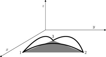
Figure 2: Coordinate system for calculation of integrals. The triangle is rotated so that the vertices 1,2,3 lie in the plane $z=0$ (shown shaded), and translated so that the field point lies at a position $(0,0,z)$.

Figure 2 shows the curved triangle in its reference position, rotated so that the corners lie in the plane $z=0$, and shifted so that the field point lies at $\mathbf{x}=(0,0,z)$. The integral to be evaluated is

$$I =\int_{0}^{1}\int_{0}^{1-\xi}f(\xi,\eta)J(\xi,\eta)\,\mathrm{d}\eta\,\mathrm{d}\xi,$$ (11)

where $J(\xi,\eta)$ is the Jacobian for the transformation from $(\xi,\eta)$ to coordinates on the element surface. Converting to Cartesian coordinates in the problem system of axes:

$$I =\int_{\triangle}f(\xi,\eta)r\,\mathrm{d}r\,\mathrm{d}\theta,$$ (12)

where integration takes place over the projection of the curved triangle into the plane $z=0$ and the function $f(\xi,\eta)$ is computed by transformation from $(r,\theta)$ to $(\xi,\eta)$.

Figure 3: Intersection of rays with curved triangle: bold lines show the part of each ray which lies inside the domain of integration.

The integration of Equation 12 is conceptually simple, and is readily applied to first order elements [6], but gives rise to some extra complexities in the second order case, shown in Figure 3. As written, the integration is composed of a sequence of integrals over $r$, along rays at fixed values of $\theta$. In Figure 3, two such rays are shown, at angles $\theta_{1}$ and $\theta_{2}$. The ray at $\theta_{1}$ presents no particular difficulties: it has one entry and one exit point on the element boundary, both easily found using analytical methods (see Section 2.3). The ray at $\theta_{2}$, however, is broken as it crosses the triangle boundary, having two entry and two exit points. In evaluating Equation 12, this case must be handled, as must the case of a ray which lies tangent to an edge. The algorithm of Section 2.4 handles these special cases, using the geometrical operations of the next section.

2.3 Geometrical operations

The quadrature algorithm, presented in Section 2.4, depends on the availability of a number of elementary geometrical operations, described in this section. These operations can be implemented analytically using standard methods and are used to determine the limits of integration in $\theta$, to break the integral at possible points of discontinuity, and in $r$, to find the entry and exit points on the triangle boundary.

The first operation is finding the intersection, $\gamma$ or $(r,\theta)$, between a ray through the origin of angle $\theta$ and an edge of the triangle. The coordinates of a point on the edge are given by Equation 9:

$$x=x_{i}J_{1}(\gamma)+x_{j}J_{2}(\gamma)+x_{i+3}J_{3}(\gamma),\,y=y_{i}J_{1}(\gamma)+y_{j}J_{2}(\gamma)+y_{i+3}J_{3}(\gamma),$$ (13)

while the ray is given by $x=r\cos\theta$, $y=r\sin\theta$, so that, upon substitution:

$$(x_{i}\sin\theta-y_{i}\cos\theta)J_{1}(\gamma)+(x_{j}\sin\theta-y_{j}\cos\theta)J_{2}(\gamma)+(x_{i+3}\sin\theta-y_{i+3}\cos\theta)J_{3}(\gamma)=0,$$ (14)

which is a quadratic in $\gamma$. To find the intersection:

1. solve Equation 14 for $\gamma$;

2. for each value of $\gamma$, with $0\leq\gamma\leq 1$

   1. compute $(x,y)$ and $r=x/\cos\theta$ or $r=y/\sin\theta$;

   2. if $r>0$, $\gamma$ is a valid intersection.

In this operation, $r$ is computed as shown in order to accept only $r>0$, to avoid double counting of intersections. The condition $0\leq\gamma\leq 1$ is imposed to exclude corners of the triangle, as these are handled separately in the algorithm.

Tangents which pass through the origin must also be determined, in order to break the integration at these points. They are found using the equation of a tangent to a point $(x_{0},y_{0})$ on the edge:

$$y =y_{0}+\left.\frac{\mathrm{d}y}{\mathrm{d}x}\right|_{x=x_{0}}(x-x_{0}),$$ (15)

$$\left.\frac{\mathrm{d}y}{\mathrm{d}x}\right|_{x=x_{0}} =\frac{y_{i}J^{\prime}_{1}(\gamma)+y_{j}J^{\prime}_{2}(\gamma)+y_{i+3}J^{\prime}_{3}(\gamma)}{x_{i}J^{\prime}_{1}(\gamma)+x_{j}J^{\prime}_{2}(\gamma)+x_{i+3}J^{\prime}_{3}(\gamma)},$$ (16)

where the prime denotes differentiation with respect to $\gamma$. Setting $x=y=0$ to find a tangent through the origin yields:

$$x_{i}y_{j}\left[J_{1}^{\prime}(\gamma)J_{2}(\gamma)-J_{2}^{\prime}(\gamma)J_{1}(\gamma)\right]+x_{j}y_{i+3}\left[J_{2}^{\prime}(\gamma)J_{3}(\gamma)-J_{3}^{\prime}(\gamma)J_{2}(\gamma)\right]$$

$$+x_{i+3}y_{i}\left[J_{3}^{\prime}(\gamma)J_{1}(\gamma)-J_{1}^{\prime}(\gamma)J_{3}(\gamma)\right]=0,$$ (17)

which is a cubic which can be solved for $\gamma$ subject to the constraint $0<\gamma<1$ and that $\gamma$ be real.

The final part of determining the limits of integration in $\theta$ is the angle $\psi$ of a tangent to an edge, given by:

$$\psi =\tan^{-1}\frac{y_{i}J^{\prime}_{1}(\gamma)+y_{j}J^{\prime}_{2}(\gamma)+y_{i+3}J^{\prime}_{3}(\gamma)}{x_{i}J^{\prime}_{1}(\gamma)+x_{j}J^{\prime}_{2}(\gamma)+x_{i+3}J^{\prime}_{3}(\gamma)},$$ (18)

from the slope of the curve at a point $\gamma$ on an edge. A second angle $\psi+\pi$ is also included in order to ensure that rays in both tangent directions are included.

2.4 Quadrature algorithm

The algorithm for the quadrature rule consists of a first stage in which the range of integration in $\theta$ is broken into a set of intervals, and a second in which the integration is performed over these intervals. Initially it must be determined whether the origin lies inside, outside or on the boundary of the triangle projected into the plane $z=0$. This is done by first checking if the origin lies outside a box containing the points $(x_{1},y_{1})$, $(x_{2},y_{2})$, and $(x_{3},y_{3})$. If not, its coordinates $(\xi,\eta)$ in the triangle are found using Newton’s method, and it is checked whether they lie within the triangle.

In the first stage of processing:

1. find possible limits of integration $\theta_{i}$, $i=1,\ldots,N$, as the angles of rays joining the origin to the triangle’s corners, the angles of tangents through the origin, and, if the origin lies on an edge, the angles of tangents to the edge;

2. adjust all angles to lie in the range $0,2\pi$;

3. sort the list of limits $\theta_{i}$ in ascending order;

4. if the origin lies inside the triangle, append the angle $\theta_{1}+2\pi$.

Given the list of $N$ angles from the first stage, the nodes and weights of the quadrature rule are found for each pair of limits, $\theta_{i}$, $\theta_{i+1}$ by this procedure:

1. select a quadrature rule with abscissae $\theta_{k}$ and weights $w_{k}^{\theta}$, $k=1,\ldots,K$;

2. for each $k$:

   1. find the radii $r_{j}$ of the intersections of a ray of angle $\theta_{k}$ with the triangle edges (prepend $r=0$ if the origin lies inside the triangle);

   2. for each pair of limits $r_{2j}$ and $r_{2j+1}$, select a quadrature rule $(r_{m},w_{m}^{r})$, $m=1,\ldots,M$;

   3. for each point $(r_{m}\cos\theta_{k},r_{m}\sin\theta_{k})$:

      1. find the corresponding coordinates $(\xi,\eta)$ using Newton’s method;

      2. append to the quadrature rule the abscissa $(\xi,\eta)$ and the weight $r_{m}w_{m}^{r}w_{k}^{\theta}/J_{2}(\xi,\eta)$, where $J_{2}$ is the Jacobian for conversion from $(\xi,\eta)$ to $(r,\theta)$.

The resulting quadrature rule can be used to evaluate an integral on the panel by summation:

$$\int_{0}^{1}\int_{0}^{1-\xi}f(\xi,\eta)J(\xi,\eta)\,\mathrm{d}\eta\,\mathrm{d}\xi \approx\sum_{n}f(\xi_{n},\eta_{n})J(\xi_{n},\eta_{n})w_{n},$$ (19)

where $J(\xi,\eta)$ is the Jacobian for conversion from $(\xi,\eta)$ to the surface coordinates $(x,y,z)$, allowing the rule to be used in the same manner as standard quadratures for triangles. We note that since the quadrature rule is mapped to the reference triangle, the sum of the weights $w_{n}$ should be equal to $1/2$, which gives a convenient error measure for checking the accuracy of the quadrature.

Finally, a good starting guess for Newton’s method in finding coordinates on the reference triangle is provided by the intersection point $(r,\theta)$ since its value of $\gamma$ on the edge is known, and can be converted to $(\xi,\eta)$ using Equation 10. Each set of coordinates $(\xi,\eta)$ on a ray can then be used as an initial guess for the evaluation at the next quadrature point.

2.5 Quadrature selection

The quadrature rule is implemented using a sequence of Gaussian quadratures for integration in $\theta$ and $r$. This has the first advantage that the endpoints of the integral are not included. Since tangents are used to fix limits of integration, there is then no ambiguity in determining the number of entry and exit points in radius.

The quadrature rules are selected using a criterion which gives some adaptivity to the intervals of integration. A point separation parameter $\Delta\theta$ is specified and used to estimate the number of points required in the quadrature rule:

$$K =\left[(\theta_{i+1}-\theta_{i})/\Delta\theta\right],$$ (20)

where $[\cdot]$ denotes rounding of the value to the nearest natural number. The resulting value $K$ is then adjusted to lie in a range $K_{\min}\leq K\leq K_{\max}$. A similar method is used to select quadrature rules in $r$. In the calculations presented here, the values of $\Delta\theta$ and $\Delta r$ are computed with user-defined constants $N_{\theta}$ and $N_{r}$, and set as follows:

$$\Delta\theta =\frac{\max_{i}\phi_{i}}{N_{\theta}},$$ (21a)

$$\Delta r =\frac{\max_{i}\ell_{i}}{N_{r}},$$ (21b)

where $\phi_{i}$ is the angle subtended by the corner of the triangle at vertex $i$, $i=1,2,3$ and $\ell_{i}$ is the length of the straight edge starting at corner $i$. This gives a quickly computed abscissa density under user control.

Finally, in using the algorithm in a code, a criterion is required in deciding when to use it, and when not. In this case, a parameter $\sigma$ is computed based on easily evaluated geometric properties of the element. These are the mean values of the nodes and the radius of a sphere containing the element:

$$\overline{\mathbf{y}} =\frac{1}{6}\sum_{i=1}^{6}\mathbf{y}_{i},$$ (22a)

$$\rho =s\max_{i}|\mathbf{y}_{i}-\overline{\mathbf{y}}|,$$ (22b)

where $s$ is a scaling factor, with, in this case, $s=2^{1/2}$. Given these values for the element, $\sigma$ is determined as follows:

1. if $\mathbf{x}$ lies on the element, $\sigma=0$;

2. compute $\rho_{x}=|\mathbf{x}-\overline{\mathbf{y}}|$: if $\rho_{x}>\rho$, $\sigma=\rho_{x}/\rho$;

3. otherwise, $\sigma=z/\rho$,

where $z$ is the distance of $\mathbf{x}$ from the element reference plane, as noted above. This gives a quickly-computed parameter which varies from $0$ on the element to large values away from the element, but remains small in some reasonable neighbourhood, so that it can be used to select quadrature methods.

3 NUMERICAL TESTS

The algorithm of the previous section is demonstrated using two sets of results. The first is an illustration of the distribution of quadrature nodes, using a sample element, while the second is an assessment of the accuracy and convergence of the method when implemented in a BEM program.

3.1 Quadrature points

Figure 4: Quadrature points for different field points: origin is shown as a cross, quadrature points as dots. Top row: origin inside element, on vertex, and outside element. Bottom row: origin on straight, convex and concave edge.

To demonstrate the nature of the quadrature point distributions generated by the algorithm, an element with one straight, one convex and one concave edge has been used, with the origin placed inside and outside the element, on a corner, and on each of the edges in turn. In order to show the point distribution more clearly, fixed length quadrature rules have been used, with sixteen points in both angle and radius. This gives a higher than normal density in small intervals of integration, and a lower density in larger regions, but is helpful for visualization.

Figure 4 shows the resulting quadratures, with the origin indicated by a cross. Each of the cases considered gives rise to a qualitatively different point distribution. With the origin located inside the element, the region of integration is divided by rays to each of the corners (compare Figure 8 of reference [9]). When the origin is placed on a corner of the element, there are two clearly demarcated domains of integration, separated by the tangent to the curved edge at that corner. Similarly, when the origin is moved outside the element, there are two domains, separated in this case by a ray joining the origin to the most distant corner.

When the origin lies on an edge, the situation is slightly more complicated. When it is on the straight edge, the element is divided into two regions, separated by the ray to the furthest corner. When it lies on the convex edge, there is a thin region of integration bounded by the edge and the rays to the vertices on that edge. Conversely, on the concave edge, the narrow region of integration is bounded by the edge and the tangent to the edge at the origin.

3.2 Numerical accuracy and convergence

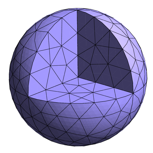
Figure 5: The cat’s eye geometry

The accuracy and convergence of the integration method are tested by implementing it in a BEM code [11] and solving the Laplace equation on a cat’s eye geometry, shown in Figure 5. This is a unit sphere with one octant removed, recommended as a more stringent test of BEM codes than a simple sphere [12], since it contains discontinuities in the geometry, as would be found, for example, in aerodynamic calculations. The surface was meshed using GMSH [13], changing the discretization length to produce panels of varying sizes. A second mesh was produced for comparison by splitting each second order element into six triangles, giving a mesh of planar elements based on the same nodes. The polar quadrature rule was selected for $\sigma<1$, with $N_{\theta}=N_{r}=8$, and a twenty-five point symmetric rule [14] for $\sigma\geq 1$.

Figure 6: Error $\epsilon$ in solution of Laplace equation on cat’s eye against panel number $P$ (upper) and node number $N$ (lower). Dots: linear elements; squares: quadratic elements. Upper plot: solid line $6.6P^{-1.1}$; dashed line: $3.9P^{-1.6}$. Lower plot: solid line $4.8N^{-1.2}$; dashed line: $19.3N^{-1.6}$.

A Neumann boundary condition was generated using a point potential source positioned inside the surface at $(-0.2,-0.2,-0.2)$. Solving Equation 1 for the surface potential $\phi$ gave a result which could be compared to the result found analytically for the point source. The error estimate is the r.m.s. difference between the computed and the analytically specified data. The error is plotted in Figure 6 as a function of element number, and, for convenience, of node number. The error is fitted using a power law, to estimate the convergence rate, and the superior numerical performance of the second order method is clear. Plotting against panel number shows a similar convergence rate as in other work [9, Figure 12], $P^{-1}$ for linear panels, and $P^{-3/2}$ for quadratic. Plotting against node number, which can be taken as a proxy for the memory requirement for the matrix used to solve the problem, and which shows error for different element types on the same point distribution, shows similar trends.

4 CONCLUSIONS

A quadrature technique for second order triangular elements has been presented and tested on a realistic geometry. It has been found that the method is accurate and convergent, giving an error which scales as $P^{-1.6}$ in the example tested. It is concluded that the technique is readily implemented and can be used as a direct replacement for existing quadratures.

References

- [1] Ephraim E. Okon and Roger F. Harrington. The potential integral for a linear distribution over a triangular domain. International Journal for Numerical Methods in Engineering, 18:1821–1828, 1982.
- [2] Ephraim E. Okon and Roger F. Harrington. The potential due to a uniform source distribution over a triangular domain. International Journal for Numerical Methods in Engineering, 18:1401–1419, 1982.
- [3] J. N. Newman. Distributions of sources and normal dipoles over a quadrilateral panel. Journal of Engineering Mathematics, 20:113–126, 1986.
- [4] J.-C. Suh. The evaluation of the Biot–Savart integral. Journal of Engineering Mathematics, 37:375–395, 2000.
- [5] A. Salvadori. Analytical integrations in 3D BEM for elliptic problems: Evaluation and implementation. International Journal for Numerical Methods in Engineering, 84:505–542, 2010.
- [6] Michael Carley. Potential integrals on triangles. Accepted for publication in ASME Journal of Applied Mechanics, 2013.
- [7] David J. Willis, Jaime Peraire, and Jacob K. White. A combined pFFT-multipole tree code, unsteady panel method with vortex particle wakes. In 43rd AIAA Aerospace Sciences Meeting, number AIAA-2005-0854, 2005.
- [8] David J. Willis, Jaime Peraire, and Jacob K. White. A combined pFFT-multipole tree code, unsteady panel method with vortex particle wakes. International Journal for Numerical Methods in Fluids, 53:1399–1422, 2007.
- [9] David J. Willis, Jaime Peraire, and Jacob K. White. A quadratic basis function, quadratic geometry, high order panel method. In 44th AIAA Aerospace Sciences Meeting, number AIAA-2006-1253, 2006.
- [10] X. Wang, J. N. Newman, and J. White. Robust algorithms for boundary-element integrals on curved surfaces. In International Conference on Modeling and Simulation of Microsystems, 2000.
- [11] Michael Carley. BEM3D: A free three-dimensional boundary element library. http://www.paraffinalia.co.uk/Software/bem3d.shtml, 2009–2013. accessed .
- [12] Steffen Marburg and Sia Amini. Cat’s eye radiation with boundary elements: Comparative study on treatment of irregular frequencies. Journal of Computational Acoustics, 13(1):21–45, 2005.
- [13] Christophe Geuzaine and Jean-François Remacle. Gmsh: a three-dimensional finite element mesh generator with built-in pre- and post-processing facilities. International Journal for Numerical Methods in Engineering, 79(11):1309–1331, 2009.
- [14] S. Wandzura and H. Xiao. Symmetric quadrature rules on a triangle. Computers and Mathematics with Applications, 45:1829–1840, 2003.