On learning parametric-output HMMs

Abstract

We present a novel approach to learning an HMM whose outputs are distributed according to a parametric family. This is done by decoupling the learning task into two steps: first estimating the output parameters, and then estimating the hidden states transition probabilities. The first step is accomplished by fitting a mixture model to the output stationary distribution. Given the parameters of this mixture model, the second step is formulated as the solution of an easily solvable convex quadratic program. We provide an error analysis for the estimated transition probabilities and show they are robust to small perturbations in the estimates of the mixture parameters. Finally, we support our analysis with some encouraging empirical results.

1 Introduction

Hidden Markov Models (HMM) are a standard tool in the modeling and analysis of time series with a wide variety of applications. When the number of hidden states is known, the standard method for estimating the HMM parameters from given observed data is the Baum-Welch algorithm (Baum et al., 1970). The latter is known to suffer from two serious drawbacks: it tends to converge (i) very slowly and (ii) only to a local maximum. Indeed, the problem of recovering the parameters of a general HMM is provably hard, in several distinct senses (Abe and Warmuth, 1992; Lyngsø and Pedersen, 2001; Terwijn, 2002).

In this paper we consider learning parametric-output HMMs with a finite and known number of hidden states, where the output from each hidden state follows a parametric distribution from a given family. A notable example is a Gaussian HMM, where from each state $x$, the output is a (possibly multivariate) Gaussian, $\mathcal{N}(\mu_{x},\Sigma_{x})$, typically with unknown $\mu_{x},\Sigma_{x}$.

Main results.

We propose a novel approach to learning parametric output HMMs, based on the following two insights: (i) in an ergodic HMM, the stationary distribution is a mixture of distributions from the parametric family, and (ii) given the output parameters, or their approximate values, one can efficiently recover the corresponding transition probabilities up to small additive error.

Combining these two insights leads to our decoupling approach to learning parametric HMMs. Rather than attempting, as in the Baum-Welch algorithm, to jointly estimate both the transition probabilities and the output density parameters, we instead learn each of them separately. First, given one or several long observed sequences, the HMM output parameters are estimated by a general purpose parametric mixture learner, such as the Expectation-Maximization (EM) algorithm. Next, once these parameters are approximately known, we learn the hidden state transition probabilities by solving a computationally efficient convex quadratic program (QP).

The key idea behind our approach is to treat the underlying hidden process as if it were sampled independently from the Markov chain’s stationary distribution, and operate only on the empirical distribution of singletons and consecutive pairs. Thus we avoid computing the exact likelihood, which depends on the full sequence, and obtain considerable gains in computational efficiency. Under mild assumptions on the Markov chain and on its output probabilities, we prove in Theorem 1 that given the exact output probabilities, our estimator for the hidden state transition matrix is asymptotically consistent. Additionally, this estimator is robust to small perturbations in the output probabilities (Theorems 2-6).

Beyond its practical prospects, our proposed approach also sheds light on the theoretical difficulty of the full HMM learning problem: It shows that for parametric-output HMMs the key difficulty is fitting a mixture model, since once its parameters have been accurately estimated, learning the transition matrix can be cast as a convex program. While learning a general mixture is considered a hard problem, we note that recently much progress has been made under various separation conditions on the mixture components, see e.g. Moitra and Valiant (2010); Belkin and Sinha (2010) and references therein.

Related work.

The problem of estimating HMM parameters from observations has been actively studied since the 1970’s, see Cappé et al. (2005); Rabiner (1990); Roweis and Ghahramani (1999). While computing the maximum-likelihood estimator for an HMM is in general computationally intractable, under mild conditions, such an estimator is asymptotically consistent and normally distributed, see Bickel et al. (1998); Chang (1996); Douc and Matias (2001).

In recent years, there has been a renewed interest in learning HMMs, in particular under various assumptions that render the learning problem tractable (Faragó and Lugosi, 1989; Hsu et al., 2009; Mossel and Roch, 2006; Siddiqi et al., 2010; Anandkumar et al., 2012). Also, Cybenko and Crespi (2011); Lakshminarayanan and Raich (2010) recently suggested Non-negative Matrix Factorization (NNMF) approaches for learning HMMs. These methods are related to our approach, since with known output probabilities, NNMF reduces to a convex program similar to the one considered here. Hence, our stability and consistency analysis may be relevant to NNMF-based approaches as well.

Paper outline.

In Section 2 we present our problem setup. The algorithm for learning the HMM appears in Section 3, and its statistical analysis in Section 4. Section 5 contains some simulation results. The technical details are deferred to the Appendices.

2 Problem Setup

Notation.

When $X\in{\mathcal{X}}$ and $Y\in{\mathcal{Y}}$ take values in a discrete set we abbreviate $P(x)$ for $\Pr(X\!=\!x)$ and $P(y\,|\,x)$ for $\Pr(Y=y\,|\,X=x)$. When $Y\in{\mathcal{Y}}$ is continuous-valued, we denote by $P(y\,|\,x)$ the probability density function of $Y$ given $X$.

For $x,w\in\mathbb{R}^{n}$, $\operatorname{diag}(x)$ denotes the $n\times n$ diagonal matrix with entries $x_{i}$ on its diagonal, $x/w$ is the vector with entries $x_{i}/w_{i}$, and $\left\|x\right\|_{w}^{2}=\sum_{i}w_{i}x_{i}^{2}$ is a $w$-weighted $\ell_{2}$ norm (for $w_{i}>0$). The shorthand $x\lesssim y$ means $x\leq(1+o(1))y$. Similarly we write $x\lesssim_{P}y$ for $x\leq(1+o_{P}(1))y$. Finally, for a positive integer $n\in\mathbb{N}$, we write $[n]=\{1,2,\ldots,n\}$.

Hidden Markov Model.

We consider a discrete-time, discrete-space HMMs with $n$ hidden states. The HMM output alphabet, denoted ${\mathcal{Y}},$ may be either discrete or continuous. A parametric-output HMM is characterized by a tuple $(A,{\mathcal{F}}_{n}^{\theta},P_{0})$ where $A$ is an $n\times n$ column stochastic matrix, $P_{0}$ is the distribution of the initial state and ${\mathcal{F}}_{n}^{\theta}=(f_{\theta_{1}},\dots,f_{\theta_{n}})$ is an ordered tuple of parametrized probability density functions. In the sequel we sometimes write $f_{i}$ instead of $f_{\theta_{i}}$.

To generate the output sequence of the HMM, first an unobserved Markov sequence of hidden states $x=\{x_{t}\}_{t=0}^{T-1}$ is generated with the following distribution.

$$P(x) = P_{0}(x_{0})\prod_{t=1}^{T-1}A_{x_{t},x_{t-1}},$$

where $A_{ij}=P(X_{t}=i\,|\,X_{t-1}=j)$ are the transition probabilities. Then, each hidden state $X_{t}$ independently emits an observation $Y_{t}\in{\mathcal{Y}}$ according to the distribution $P(y_{t}\,|\,x_{t})\equiv f_{x_{t}}(y_{t})$. Hence the output sequence $y=(y_{t})_{t=0}^{T-1}$ has the conditional probability

$$P(y\,|\,x)=\prod_{t=0}^{T-1}P(y_{t}\,|\,x_{t})=\prod_{t=0}^{T-1}f_{x_{t}}(y_{t}).$$

The HMM Learning Problem.

Given one or several HMM output sequences $(Y_{t})_{t=0}^{T-1}$, the HMM learning problem is to estimate both the transition matrix $A$ and the parameters of the output distributions ${\mathcal{F}}_{n}^{\theta}$.

3 Learning Parametric-Output HMMs

The standard approach to learning the parameters of an HMM is to maximize the likelihood

$$\sum_{x\in[n]^{T}}\!P_{0}(x_{0})P(y_{0}\,|\,x_{0})\prod_{t=1}^{T-1}A_{x_{t},x_{t-1}}P(y_{t}\,|\,x_{t}).$$

As discussed in the Introduction, this problem is in general computationally hard. In practice, neglecting the small effect of the initial distribution $P_{0}(x_{0})$ on the likelihood, $A$ and ${\mathcal{F}}_{n}^{\theta}$ are usually estimated via the Baum-Welch algorithm, which is computationally slow and only guaranteed to converge to a local maximum.

3.1 A Decoupling Approach

In what follows we show that when the output distributions are parametric, we can decouple the HMM learning task into two steps: learning the output parameters $\theta_{1},\ldots,\theta_{n}$ followed by learning the transition probabilities of the HMM. Under some mild structural assumptions on the HMM, this decoupling implies that the difficulty of learning a parametric-output HMM can be reduced to that of learning a parametric mixture model. Indeed, given (an approximation to) ${\mathcal{F}}_{n}^{\theta}$’s parameters, we propose an efficient, single-pass, statistically-consistent algorithm for estimating the transition matrix $A$.

As an example, consider learning a Gaussian HMM with univariate outputs. While the Baum-Welch approach jointly estimates $n^{2}+2n$ parameters (the matrix $A$ and the parameters $\mu_{i},\sigma_{i}^{2}$), our decoupling approach first fits a mixture model with only $3n$ parameters $(\pi_{i},\mu_{i},\sigma_{i}^{2})$, and then solves a convex problem for the matrix $A$. While both problems are in general computationally hard, ours has a significantly lower dimensionality for large $n$.

Assumptions.

To recover the matrix $A$ and the output parameters $\theta_{j}$ we make the following assumptions:

(1a) The Markov chain has a unique stationary distribution $\boldsymbol{\pi}$ over the $n$ hidden states. Moreover, each hidden state is recurrent with a frequency bounded away from zero: $\min_{k}\pi_{k}\geq a_{0}$ for some constant $a_{0}>0$.

(1b) The $n\times n$ transition matrix $A$ is geometrically ergodic: there exists parameters $G<\infty$ and $\psi\in[0,1)$ such that from any initial distribution $P_{0}$

$$\left\|A^{t}P_{0}-\boldsymbol{\pi}\right\|_{1}\leq 2G\psi^{t},\qquad\forall t\in\mathbb{N}.$$ (1)

(1c) The output parameters of the $n$ states are all distinct: $\theta_{i}\neq\theta_{j}$ for $i\neq j$. In addition, the parametric family is identifiable.

Remarks:

Assumption (1a) rules out transient states, whose presence makes it generally impossible to estimate all entries in $A$ from one or a few long observed sequences. Assumption (1b) implies mixing and is used later on to bound the error and the number of samples needed to learn the matrix $A.$ Assumption (1c) is crucial to our approach, which uses the distribution of only single and pairs of consecutive observations. If two states $i,j$ had same output parameters, it would be impossible to distinguish between them based on single outputs.

3.2 Learning the output parameters.

Assumptions (1a,1b) imply that the Markov chain over the hidden states is mixing, and so after only a few time steps, the distribution of $X_{t}$ is very close to stationary. Assuming for simplicity that already $X_{0}$ is sampled from the stationary distribution, or alternatively neglecting the first few outputs, this implies that each observable $Y_{t}$ is a random realization from the following parametric mixture model,

$$Y\sim\sum_{i=1}^{n}\pi_{i}f_{\theta_{i}}(y).$$ (2)

Hence, given the output sequence $(Y_{t})_{t=0}^{T-1}$ one may estimate the output parameters $\theta_{i}$ and the stationary distribution $\pi_{i}$ by fitting a mixture model of the form (2) to the observations. This is commonly done via the EM algorithm.

Like its more sophisticated cousin Baum-Welch, the mixture-learning EM algorithm also suffers from local maxima. Indeed, from a theoretical viewpoint, learning such a mixture model (i.e. the parameters of ${\mathcal{F}}_{n}^{\theta}$) is a non-trivial task considered in general to be computationally hard. Nonetheless, under various separation assumptions, efficient algorithms with rigorous guarantees have been recently proposed (see e.g. Belkin and Sinha (2010)). Note that while these algorithms have polynomial complexity in sample size and output dimension, they are still exponential in the number of mixture components (i.e., in the number of hidden states of the HMM). Hence, these methods do not imply polynomial learnability of parametric-output HMMs.

In what follows we assume that using some mixture-learning procedure, the output parameters $\theta_{j}$ have been estimated with a relatively small error (say $|\hat{\theta}_{j}-\theta_{j}|=O(1/\sqrt{T})$). Furthermore, to allow for cases where $\theta_{j}$ were estimated from separate observed sequences of perhaps other HMMs with same output parameters but potentially different stationary distributions, we do not assume that $\pi_{i}$ have been estimated.

3.3 Learning the transition matrix $A$

Next, we describe how to recover the matrix $A$ given either exact or approximate knowledge of the HMM output probabilities. For clarity and completeness, we first give an estimation procedure for the stationary distribution $\pi$.

Discrete observations.

As a warm-up to the case of continuous outputs, we start with HMMs with a discrete observation space of size $|{\mathcal{Y}}|=m$. In this case we can replace ${\mathcal{F}}_{n}^{\theta}$ by an $m\times n$ column-stochastic matrix $B$ such that $B_{ki}\equiv P(k\,|\,i)$ is the probability of observing an output $k$ given that the Markov chain is in hidden state $i$. In what follows, we assume that the number of output states is larger or equal to the number of hidden states, $m\geq n$, and that the $m\times n$ matrix $B$ has full rank $n$. The latter is the discrete analogue of assumption (1c) mentioned above.

First note that since the matrix $A$ has a stationary distribution $\boldsymbol{\pi}$, the process $Y_{t}$ also has a stationary distribution $\boldsymbol{\rho}$, which by analogy to Eq. (2), is

$$\boldsymbol{\rho}=B\boldsymbol{\pi}.$$ (3)

Similarly, the pair $(Y_{t},Y_{t+1})$ has a unique stationary distribution ${\boldsymbol{\sigma}}$, given by

$$\sigma_{k,k^{\prime}} = \sum_{\ell,\ell^{\prime}\in[n]}\pi_{\ell}A_{\ell^{\prime},\ell}B_{k,\ell}B_{k^{\prime},\ell^{\prime}}.$$ (4)

As we shall see below, knowledge of $\boldsymbol{\rho}$ and $\boldsymbol{\sigma}$ suffices to estimate $\boldsymbol{\pi}$ and $A$. Although $\boldsymbol{\rho}$ and $\boldsymbol{\sigma}$ are themselves unknown, they are easily estimated from a single pass on the data $(Y_{t})_{t=0}^{T-1}$:

$$\hat{\rho}_{k} = \frac{1}{T}\sum_{t=0}^{T-1}\boldsymbol{\mathbbm{1}}_{\left\{y_{t}=k\right\}},$$

$$\hat{\sigma}_{k,k^{\prime}} = \frac{1}{T-1}\sum_{t=1}^{T-1}\boldsymbol{\mathbbm{1}}_{\left\{y_{t-1}=k\right\}}\boldsymbol{\mathbbm{1}}_{\left\{y_{t}=k^{\prime}\right\}}.$$ (5)

Estimating the stationary distribution $\boldsymbol{\pi}$.

The key idea in our approach is to replace the exact, but complicated and non-convex likelihood function by a “pseudo-likelihood”, which treats the hidden state sequence $(X_{t})$ as if they were iid draws from the unknown stationary distribution $\boldsymbol{\pi}$. The pseudo-likelihood has the advantage of having an easily computed global maximum, which, as we show in in Section 4, yields an asymptotically consistent estimator. Approximating the $(X_{t})$ as iid draws from $\boldsymbol{\pi}$ means that the $(Y_{t})$ are treated as iid draws from $\boldsymbol{\rho}=B\boldsymbol{\pi}$. Thus, given a sequence $(Y_{t})_{t=0}^{T-1}$ the pseudo-likelihood for a vector $\boldsymbol{\pi}$ is

$$\mathcal{L}(y_{0},\ldots,y_{T-1}\,|\,\boldsymbol{\pi})=\prod_{i=0}^{T-1}(B\boldsymbol{\pi})_{y_{i}}=\prod_{k=1}^{m}(B\boldsymbol{\pi})_{k}^{n_{k}}$$

where $n_{k}=\sum_{i=0}^{T-1}\boldsymbol{\mathbbm{1}}_{\left\{y_{t}=k\right\}}=T\hat{\rho}_{k}$. Its maximizer is

$$\hat{\boldsymbol{\pi}}^{\textrm{{\tiny{ML}}}}=\underset{x_{i}\geq 0,\,\|x\|_{1}=1}{\arg\min}-\sum_{k=1}^{m}\hat{\rho}_{k}\log(Bx)_{k}.$$ (6)

Since $-\log(x)$ is convex, $(Bx)_{k}$ is a linear combination of the unknown variables $x_{j}$, and the constraints are all linear, the above is nothing but a convex program, easily solved via standard optimization methods (Nesterov and Nemirovskii, 1994).

However, to facilitate the analysis and to increase the computational efficiency, we consider the asymptotic behavior of the pseudo-likelihood in (6), for $T$ sufficiently large so that $\hat{\boldsymbol{\rho}}$ is close to $\boldsymbol{\rho}$. First, we write

$$(Bx)_{k}=\hat{\rho}_{k}\left(1+\frac{(Bx)_{k}-\hat{\rho}_{k}}{\hat{\rho}_{k}}\right).$$

Next, assuming that $T\gg 1$ is sufficiently large to ensure $|(Bx)_{k}-\hat{\rho}_{k}|\ll\hat{\rho}_{k}$, we take a second order Taylor expansion of $\log(Bx)_{k}$ in (6). This gives

$$-\sum_{k=1}^{n}\hat{\rho}_{k}\log\hat{\rho}_{k}-\sum_{k=1}^{n}((Bx)_{k}-\hat{\rho}_{k})+$$

$$\quad+\sum_{k=1}^{n}\hat{\rho}_{k}\left(\frac{(Bx)_{k}-\hat{\rho}_{k}}{\hat{\rho}_{k}}\right)^{2}+O\left(\frac{\left\|Bx-\hat{\boldsymbol{\rho}}\right\|_{\infty}^{3}}{\min_{j}\rho_{j}^{2}}\right).$$

The first term is independent of $x$, whereas the second term vanishes. Thus, we may approximate (6) by the quadratic program

$$\underset{x_{i}\geq 0,\,\|x\|_{1}=1}{\mathop{\mathrm{argmin}}}{\|\hat{\boldsymbol{\rho}}-Bx\|^{2}_{(1/\hat{\boldsymbol{\rho}})}}$$ (7)

where $\|x\|_{w}^{2}=\sum_{k}w_{k}x_{k}^{2}$ is a weighted $\ell_{2}$ norm w.r.t. the weight vector $w$. Eq. (7) is also a convex problem, easily solved via standard optimization techniques. However, let us temporarily ignore the non-negativity constraints $x_{i}\geq 0$ and add a Lagrange multiplier for the equality constraint $\sum x_{i}=1$:

$$\min\frac{1}{2}\sum_{k=1}^{m}\frac{1}{\hat{\rho}_{k}}\Big{(}\hat{\rho}_{k}-\sum_{j=1}^{n}B_{kj}x_{j}\Big{)}^{2}-\lambda\Big{(}\sum_{j}x_{j}-1\Big{)}.$$ (8)

Differentiating with respect to $x_{i}$ yields

$$Wx=(1+\lambda)\boldsymbol{1},$$ (9)

where $W=B^{\intercal}\!\operatorname{diag}(1/\hat{\boldsymbol{\rho}})B$. Enforcing the normalization constraint is equivalent to solving for $x^{*}=W^{-1}\boldsymbol{1}$ and normalizing $\hat{\boldsymbol{\pi}}=x^{*}/\left\|x^{*}\right\|_{1}$. Note that if all entries of $x^{*}$ are positive, $\hat{\boldsymbol{\pi}}$ is the solution of the optimization problem in (7), and we need not invoke a QP solver. Assumptions (1a,1b) that $\pi_{k}$ is bounded away from zero and that the chain is mixing imply that for sufficiently large $T$, all entries of $\hat{\boldsymbol{\pi}}$ will be positive with high probability, see Section 4.

Estimating the transition matrix $A$.

To estimate $A$, we consider pairs $(Y_{t},Y_{t+1})$ of consecutive observations. By definition we have that for a single pair,

$$P(Y_{t}=k,Y_{t+1}=k^{\prime})=\sum_{i,j}B_{k^{\prime}i}B_{kj}A_{ij}P(X_{t}=j).$$

As above, we treat the $T-1$ consecutive pairs $(Y_{t},Y_{t+1})$ as independent of each other, with the hidden state $X_{t}$ sampled from the stationary distribution $\boldsymbol{\pi}$. When the output probability matrix $B$ and the stationary distribution $\boldsymbol{\pi}$ are both known, the pseudo-likelihood is given by

$$\mathcal{L}(y\,|\,A)=\prod_{(k,k^{\prime})}\Big{(}\sum_{ij}B_{k^{\prime}i}B_{kj}A_{ij}\pi_{j}\Big{)}^{n_{kk^{\prime}}},$$

where $n_{kk^{\prime}}\!=\!\sum_{t=1}^{T-1}\boldsymbol{\mathbbm{1}}_{\left\{y_{t-1}=k\right\}}\boldsymbol{\mathbbm{1}}_{\left\{y_{t}=k^{\prime}\right\}}\!=\!(T-1)\hat{\sigma}_{kk^{\prime}}$. The resulting estimator is

$$\underset{A_{ij}\geq 0,\sum_{i}A_{ij}=1,A\boldsymbol{\pi}=\boldsymbol{\pi}}{\mathop{\mathrm{argmin}}}{-\sum\hat{\sigma}_{kk^{\prime}}\log\Big{(}\sum_{ij}C_{ij}^{kk^{\prime}}A_{ij}\Big{)}}$$ (10)

where $C_{ij}^{kk^{\prime}}=\pi_{j}B_{kj}B_{k^{\prime}i}$. In practice, since $\boldsymbol{\pi}$ is not known, we use $\hat{C}_{ij}^{kk^{\prime}}=\hat{\pi}_{j}B_{kj}B_{k^{\prime}i}$, with $\hat{\boldsymbol{\pi}}$ instead of $\boldsymbol{\pi}$. Again, (10) is a convex program in $A$ and may be solved by standard constrained convex optimization methods. To obtain a more computationally efficient formulation, let us assume that $\min_{k,k^{\prime}}\sigma_{k,k^{\prime}}\geq a_{2}>0$, and that $\min_{k,k^{\prime}}T\hat{\sigma}_{kk^{\prime}}\gg 1$, so that $|(\hat{C}A)_{kk^{\prime}}-\hat{\sigma}_{kk^{\prime}}|\ll\hat{\sigma}_{kk^{\prime}}$, where $(\hat{C}A)_{kk^{\prime}}=\sum_{ij}\hat{C}_{ij}^{kk^{\prime}}A_{ij}$. Then, as above, the approximate minimization problem is

$$\underset{A_{ij}\geq 0,\sum_{i}A_{ij}=1,A\hat{\boldsymbol{\pi}}=\hat{\boldsymbol{\pi}}}{\mathop{\mathrm{argmin}}}{\left\|\hat{\boldsymbol{\sigma}}-\hat{C}A\right\|_{1/\hat{\boldsymbol{\sigma}}}^{2}}.$$ (11)

In contrast to the estimation of $\boldsymbol{\pi}$, where we could ignore the non-negativity constraints, here the constraints $A_{ij}\geq 0$ are essential, since for realistic HMMs, some entries in $A$ might be strictly zero. Finally, note that if $\hat{\boldsymbol{\pi}}=\boldsymbol{\pi}$ and $\hat{\boldsymbol{\sigma}}=\boldsymbol{\sigma}$, the true matrix $A$ satisfies $\boldsymbol{\sigma}=CA$ and is the minimizer of (10).

In summary, given one or more output sequences $(y_{t})_{t=0}^{T-1}$ and an estimate of $B,$ we first make a single pass over the data and construct the estimators $\hat{\boldsymbol{\rho}}$ and $\hat{\boldsymbol{\sigma}}$, with complexity $O(T)$. Then, the stationary distribution $\boldsymbol{\pi}$ is estimated via (9), and its transition matrix $A$ via (11). To estimate $A$, we first compute the matrix product $\hat{C}^{\intercal}\hat{C}$, with $O(n^{4}m^{2})$ operations. The resulting QP has size $n^{2}$, and is thus solvable (den Hertog, 1994) in time $O(n^{6})$ — which is dominated by $O(n^{4}m^{2})$ since $m\geq n$ by assumption. Hence, the overall time complexity of estimating $A$ is $O(T+n^{4}m^{2})$.

Extension to continuous observations.

We now extend the above results to the case of continuous outputs distributed according to a known parametric family. Recall that in this case, each hidden state $i\in[n]$ has an associated output probability density $f_{\theta_{i}}(y)$. As with discrete observations, we assume that an approximation $(\hat{\theta}_{1},\dots,\hat{\theta}_{n})$ to $f_{i}$’s parameters is given and use it to construct estimates of $\boldsymbol{\pi}$ and $A$.

To this end, we seek analogues of (3) and (4), which relate the observable quantities to the latent ones. This will enable us to construct the appropriate empirical estimates and the corresponding quadratic programs, whose solutions will be our estimators $\hat{\boldsymbol{\pi}}$ and $\hat{A}$. To handle infinite output alphabets, we map each observation $y$ to an $n$-dimensional vector $\varphi(y)=(f_{\theta_{1}}(y),\ldots,f_{\theta_{n}}(y))$, whose entries are the likelihood of $y$ from each of the underlying hidden states. As shown below, this allows us to reduce the problem to a discrete “observation” space which can be solved by the methods introduced in the previous subsection.

Estimating the stationary distribution $\boldsymbol{\pi}$.

To obtain an analogue of (3), we define the vector $\boldsymbol{\xi}\in\mathbb{R}^{n}$, and matrix $K\in\mathbb{R}^{n\times n}$, which will play the role of $\boldsymbol{\rho}$ and $B$ for discrete output alphabets. The vector $\boldsymbol{\xi}$ is defined as $\boldsymbol{\xi}=\text{{\bf{E}}}[\varphi(Y)]$, or more explicitly,

$$\xi_{k} \equiv \text{{\bf{E}}}[f_{k}(Y)]=\sum_{j=1}^{n}\pi_{j}\int_{\mathcal{Y}}f_{k}(y)P(y\,|\,j)dy.$$

Similarly, the $(i,j)$ entry of $K$ is given by

$$K_{ij}\equiv\text{{\bf{E}}}[f_{i}(Y)\,|\,X=j]=\int_{\mathcal{Y}}f_{i}(y)P(y\,|\,j)dy.$$ (12)

With these definitions we have, as in Eq. (3),

$$\boldsymbol{\xi}=K\boldsymbol{\pi}.$$ (13)

Thus, given an observed sequence $(y_{t})_{t=0}^{T-1}$ we construct the empirical estimate

$$\hat{\xi}_{k}=\frac{1}{T}\sum_{t=0}^{T-1}f_{k}(y_{t}),$$ (14)

and consequently solve the QP

$$\hat{\boldsymbol{\pi}}=\underset{\left\|x\right\|_{1}=1,x\geq 0}{\arg\!\min}\left\|\hat{\boldsymbol{\xi}}-Kx\right\|_{1/\hat{\boldsymbol{\xi}}}^{2}.$$ (15)

In analogy to the discrete case, we assume $\operatorname{rank}(K)=n$ so (15) has a unique solution. Its asymptotic consistency and accuracy are discussed in Section 4.

Estimating the transition matrix $A$.

Next, following the same paradigm we obtain an analogue of (4). Bayes rule implies that for stationary chains,

$$P(k\,|\,Y)=\frac{f_{k}(Y)\pi_{k}}{\sum_{l=1}^{n}{f_{l}(Y)\pi_{l}}}.$$ (16)

We define the matrices $\boldsymbol{\eta}\in\mathbb{R}^{n\times n}$ and $F\in\mathbb{R}^{n\times n}$ (analogues of $\boldsymbol{\sigma}$ and $B$) as follows. Let $Y$ and $Y^{\prime}$ be two consecutive observations of the HMM, then

$$\eta_{kk^{\prime}} \!\!\equiv\!\! \text{{\bf{E}}}\left[P(k\,|\,Y)P(k^{\prime}\,|\,Y^{\prime})\right]$$

$$F_{kj} \!\!\equiv\!\! \text{{\bf{E}}}[P(k\,|\,Y)\,|\,j]\!=\!\!\int_{\mathcal{Y}}P(k\,|\,y)P(y\,|\,j)dy.$$ (17)

A simple calculation shows that, as in (4),

$$\eta_{kk^{\prime}}=\sum_{i,j=1}^{n}F_{k^{\prime}i}F_{kj}A_{ij}\pi_{j}.$$ (18)

Since here $F$ plays the role of $B,$ we may call it an effective observation matrix. This suggests estimating $A$ with the same tools used in the discrete case. Thus, given an observed sequence $(y_{t})_{t=0}^{T-1}$ we construct an empirical estimate $\hat{\boldsymbol{\eta}}$ by

$$\hat{\eta}_{kk^{\prime}} = \frac{1}{T-1}\sum_{t=1}^{T-1}\hat{P}(k\,|\,y_{t-1})\hat{P}(k^{\prime}\,|\,y_{t}),$$ (19)

where $\hat{P}$ is given by (16) but with $\pi$ replaced by $\hat{\pi}$. Consequently we solve the following QP

$$\hat{A}=\underset{A_{ij}\geq 0,\sum_{i}A_{ij}=1,A\hat{\boldsymbol{\pi}}=\hat{\boldsymbol{\pi}}}{\arg\!\min}\left\|\hat{\boldsymbol{\eta}}-(\hat{C}A)\right\|_{1/\hat{\boldsymbol{\eta}}}^{2},$$ (20)

where $\hat{C}_{ij}^{kk^{\prime}}=\hat{\pi}_{j}F_{kj}F_{k^{\prime}i}$ and $(\hat{C}A)_{kk^{\prime}}=\sum_{ij}\hat{C}_{ij}^{kk^{\prime}}A_{ij}$. As for the matrix $B$ in the discrete case, to ensure a unique solution to Eq. (20) we assume $\operatorname{rank}(F)=n.$

Remark 1.

Instead of (18), we could estimate $\eta^{\prime}_{k,k^{\prime}}\equiv\text{{\bf{E}}}[f_{k}(Y)f_{k^{\prime}}(Y^{\prime})]$, from which $A$ can also be recovered, since

$$\eta^{\prime}_{k,k^{\prime}}=\sum_{i,j=1}^{n}K_{k^{\prime}i}K_{kj}A_{ij}\pi_{j}.$$

This has the advantage that for many distributions the matrix $K$ can be cast in a closed analytic form. For example in the Gaussian case, while $F$ needs to be calculated numerically, we have

$$K_{ij}=\frac{1}{\sqrt{2\pi}}\frac{1}{\sqrt{\sigma_{i}^{2}+\sigma_{j}^{2}}}\exp\left(-\frac{1}{2}\frac{(\mu_{i}-\mu_{j})^{2}}{\sigma_{i}^{2}+\sigma_{j}^{2}}\right).$$

Additionally, $K$ does not depend on the stationary distribution. The drawback is that in principle, and as simulations suggest, accurately estimating $\boldsymbol{\eta}^{\prime}$ may require many more samples, see Appendix for details.

In summary, given approximate output parameters $(\hat{\theta}_{1},\dots,\hat{\theta}_{n})$, we first calculate the $n\times n$ matrix $K$. Next, we construct the vector $\hat{\boldsymbol{\xi}}$ by a single pass over the data $(Y_{t})_{t=0}^{T-1}$. Then the stationary distribution $\boldsymbol{\pi}$ is estimated via (15). Given $\hat{\boldsymbol{\pi}}$, we calculate the $n\times n$ matrix $F$, construct the empirical estimate $\hat{\boldsymbol{\eta}}$, and estimate $A$ via (20). As in the discrete observation case, the time complexity of this scheme is $O(T+n^{6})$ with additional terms for calculating $K$ and $F$.

4 Error analysis

First, we study the statistical properties of our estimators under the assumption that the output parameters, $({\theta}_{1},\dots,{\theta}_{n})$ in the continuous case, or the matrix $B$ in the discrete case, are known exactly. Later on we show that our estimators are stable to perturbations in these parameters. For simplicity, throughout this section we assume that the initial hidden state $X_{0}$ is sampled from the stationary distribution $\boldsymbol{\pi}$. This assumption is not essential and omitting it would not qualitatively change our results. All proofs are deferred to the Appendices.

To provide bounds on the error and required sample size we make the following additional assumptions:

(2a) In the discrete case, there exists an $a_{1}>0$ such that $\min_{j}\rho_{j}\geq a_{1}$.

(2b) In the continuous case, all $f_{\theta_{i}}$ are bounded:

$$\max_{i\in[n]}\sup_{y\in\mathbb{R}}f_{\theta_{i}}(y)\leq L<\infty.$$

Finally, for ease of notation we define

$$g_{\psi}\equiv\frac{2G}{1-\psi}.$$

Asymptotic Strong Consistency.

Our first result shows that with perfectly known output probabilities, as $T\to\infty$, our estimates $\hat{\boldsymbol{\pi}},\hat{A}$ are strongly consistent.

Theorem 1.

Let $(Y_{t})_{t=0}^{T-1}$ be an observed sequence of an HMM, whose Markov chain satisfies Assumptions (1a,1b). Assume $\operatorname{rank}(B)=n$ in the discrete case, or $\operatorname{rank}(F)=\operatorname{rank}(K)=n$ in the continuous case. Then, both estimators, $\hat{\boldsymbol{\pi}}$ of (9) and $\hat{A}$ of (11) in the discrete case, or (15) and (20) in the continuous case, are asymptotically strongly consistent. Namely, as $T\to\infty$, with probability one,

$$\hat{\boldsymbol{\pi}}\to\boldsymbol{\pi}\quad\mbox{and}\quad\hat{A}\to A.$$

Error analysis for the stationary distribution $\boldsymbol{\pi}$.

Recall that to estimate $\boldsymbol{\pi}$ in the discrete case, we argued that for sufficiently large sample size $T$, the positivity constraints can be ignored, which amounts to solving an $n\times n$ system of linear equations, Eq. (9). The following theorem provides both a lower bound on the required sample size $T$ for this condition to hold with high probability, as well as error bounds on the difference $\hat{\boldsymbol{\pi}}-\boldsymbol{\pi}$.

Theorem 2.

Discrete case: Let $\hat{\boldsymbol{\rho}}$ be given by (5), and $\hat{\boldsymbol{\pi}}$ be the solution of (9). Let $\tilde{B}=\operatorname{diag}(1/\sqrt{\boldsymbol{\rho}})B$, and $\sigma_{1}(\tilde{B})$ be its smallest singular value. Under Assumption (2a), a sequence of length

$$T\gtrsim\frac{g_{\psi}\sqrt{\log n}}{a_{0}a_{1}\sigma_{1}(\tilde{B})},$$ (21)

is sufficient to ensure that with high probability, all entries in $\hat{\boldsymbol{\pi}}$ are strictly positive. Furthermore, as $T\to\infty$,

$$\left\|\hat{\boldsymbol{\pi}}-\boldsymbol{\pi}\right\|_{2}\lesssim_{P}\sqrt{\frac{g_{\psi}^{2}}{Ta_{1}^{2}\sigma_{1}^{2}(\tilde{B})}}.$$ (22)

Next we consider the errors in the estimate $\hat{\boldsymbol{\pi}}$ for the continuous observations case. For simplicity, instead of analyzing the quadratic program (15) with a weighted $\ell_{2}$ norm, we consider the following quadratic program, whose solution is also asymptotically consistent:

$$\min_{x\geq 0,\sum_{i}x_{i}=1}\|\hat{\boldsymbol{\xi}}-Kx\|^{2}_{2}.$$ (23)

This allows for a cleaner analysis, without changing the qualitative flavor of the results.

Theorem 3.

Continuous case: Let $\hat{\boldsymbol{\xi}}$ be given by (14), $\hat{\boldsymbol{\pi}}$ be the solution of (15), and $\tilde{K}=\operatorname{diag}(1/\sqrt{\boldsymbol{\xi}})K.$ Under Assumption (2b), as $T\to\infty$,

$$\left\|\hat{\boldsymbol{\pi}}-\boldsymbol{\pi}\right\|_{2}\lesssim_{P}\sqrt{\frac{(n^{3}\ln n)g_{\psi}^{2}L^{4}}{T\sigma_{1}^{4}(\tilde{K})}},$$ (24)

Error Analysis for the Matrix $A$.

Again, for simplicity, instead of analyzing the quadratic programs (11) and (20) with a weighted $\ell_{2}$ norm, we consider the following quadratic programs, whose solutions are also asymptotically consistent for $\hat{\boldsymbol{\nu}}\in\{\hat{\boldsymbol{\sigma}},\hat{\boldsymbol{\eta}}\}$:

$$\min_{A_{ij}\geq 0,\sum_{i}A_{ij}=1}\|\hat{\boldsymbol{\nu}}-\hat{C}A\|^{2}_{2}.$$ (25)

Note that this QP is applicable even if $\nu_{kk^{\prime}}=0$ for some $k,k^{\prime}$, which implies that $\hat{\nu}_{kk^{\prime}}=0$ as well.

Theorem 4.

Discrete case. Let $\hat{A}$ be the solution of (25) with $\hat{\boldsymbol{\nu}}=\hat{\boldsymbol{\sigma}}$ given in (5). Then, as $T\to\infty$,

$$\left\|\hat{A}-A\right\|_{F}\lesssim_{P}\sqrt{\frac{n^{3}g_{\psi}^{2}}{Ta_{0}^{4}a_{1}^{2}\sigma_{1}^{10}(B)}}$$ (26)

and thus an observed sequence length

$$T\gtrsim\frac{n^{3}g_{\psi}^{2}}{a_{0}^{4}a_{1}^{2}\sigma_{1}^{10}(B)}$$ (27)

suffices for accurate estimation.

Theorem 5.

Continuous case. Let $\hat{A}$ be the solution of (25) with $\hat{\boldsymbol{\nu}}=\hat{\boldsymbol{\eta}}$ given in (19). Then, as $T\to\infty$,

$$\left\|\hat{A}-A\right\|_{F}\lesssim_{P}\sqrt{\frac{(n^{7}\ln n)g_{\psi}^{2}L^{4}}{Ta_{0}^{6}\sigma_{1}^{8}(F)\sigma_{1}^{4}(K)}}$$ (28)

and thus an observed sequence length

$$T\gtrsim\frac{(n^{7}\ln n)g_{\psi}^{2}L^{4}}{a_{0}^{4}\sigma_{1}^{8}(F)\sigma_{1}^{4}(K)}$$ (29)

suffices for accurate estimation.

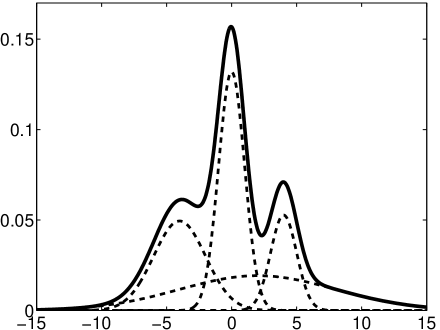
Figure 1: The mixture and its components.

Remarks. Note the key role of the smallest singular value $\sigma_{1}$, in the error bounds in the theorems above: Two hidden states with very similar output probabilities drive $\sigma_{1}$ to zero, thus requiring many more observations to resolve the properties of the underlying hidden sequence.

Inaccuracies in the output parameters.

In practice we only have approximate output parameters, found for example, via an EM algorithm. For simplicity, we study the effect of such inaccuracies only in the continuous case. Similar results hold in the discrete case. To this end, assume the errors in the matrices $K$ and $F$ of Eqs. (12) and (17) are of the form

$$\tilde{K}=K+\epsilon LQ,\quad\quad\tilde{F}=F+\epsilon P,$$ (30)

with $\left\|Q\right\|_{F},\left\|P\right\|_{F}\leq 1$. The following theorem shows our estimators are stable w.r.t. errors in the estimated output parameters. Note that if $K,F$ are estimated by a sequence of length $T$, then typically $\epsilon=O(T^{-1/2})$.

Theorem 6.

Given an error of $\epsilon$ in the output parameters as in Eq. (30), the estimators given in Theorems 3 and 5, incur an additional error of at most

$$O\left(\frac{n^{r}\epsilon}{a_{0}^{2}\sigma_{1}^{4}}\right),$$ (31)

with $r=1$ for estimating $\boldsymbol{\pi}$, and $r=\frac{3}{2}$ for estimating $A$, and where $\sigma_{1}$ is the smallest singular value of $K/L^{2}$ when estimating $\boldsymbol{\pi}$, and of $F$ when estimating $A$.

5 Simulation Results

We illustrate our algorithm by some simulation results, executed in MATLAB with the help of the HMM and EM toolboxes. We consider a toy example with $n=4$ hidden states, whose outputs are univariate Gaussians, $\mathcal{N}(\mu_{i},\sigma_{i}^{2})$, with $A$, ${\mathcal{F}}_{n}^{\theta}$ and $\boldsymbol{\pi}$ given by

$$A\! \!=\!\left(\begin{array}[]{cccc}0.7&0.0&0.2&0.5\\ 0.2&0.6&0.2&0.0\\ 0.1&0.2&0.6&0.0\\ 0.0&0.2&0.0&0.5\end{array}\right),\quad\begin{array}[]{rcl}f_{1}&=&\mathcal{N}(-4,4)\\ f_{2}&=&\mathcal{N}(0,1)\\ f_{3}&=&\mathcal{N}(2,36)\\ f_{4}&=&\mathcal{N}(4,1)\end{array}$$

$$\boldsymbol{\pi}^{\intercal}=(0.3529,0.2941,0.2353,0.1176).$$

Fig. 1 shows the mixture and its four components.

To estimate $A$ we considered the following methods:

	method	initial $\theta$	initial $A$
1	BW	random	random
2	none	exactly known	QP
3	none	EM	QP
4	BW	exactly known	QP
5	BW	EM	QP
6	BW	exactly known	random
7	BW	EM	random

Fig. 2 (left) shows on a logarithmic scale ${\text{{\bf{E}}}\|\hat{A}-A\|_{F}^{2}}$ vs. sample size $T$, averaged over 100 independent realizations. Fig. 2 (right) shows the running time as a function of $T$. In these two figures, the number of iterations of the BW step was set to 20.

Fig. 3 (left) shows the convergence of ${\text{{\bf{E}}}\|\hat{A}-A\|_{F}^{2}}$ as a function of the number of BW iterations, with known output parameters, but either with or without the QP results. Fig. 3 (right) gives ${\text{{\bf{E}}}\|\hat{A}-A\|_{F}^{2}}$ as a function of the number of BW iterations for both known and EM-estimated output parameters with $10^{5}$ samples.

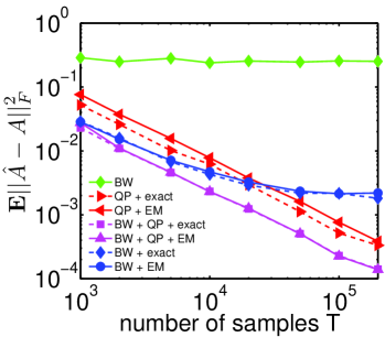
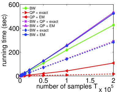
Figure 2: Average Error $\text{{\bf{E}}}\|\hat{A}-A\|_{F}^{2}$ and runtime comparison of different algorithms vs. sample size $T$.

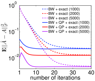
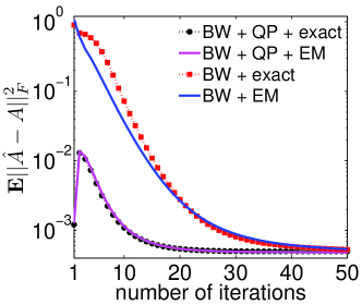
Figure 3: Convergence of the BW iterations.

The simulation results highlight the following points: (i) BW with a random guess of both $A$ and the parameters $\theta_{j}=(\mu_{j},\sigma_{j}^{2})$ is useless if run for only 20 iterations. It often requires hundreds of iterations to converge, in some cases to a poor inaccurate solution (results not shows due to lack of space); (ii) For a small number of samples the accuracy of QP+EM (method 3) is comparable to BW+EM (method 5) but requires only a fraction of the computation time. (iii) When the number of samples becomes large, the QP+EM is not only faster, but (surprisingly) also more accurate than BW+EM. As Fig. 3 suggests, this is due to the slow convergence of the BW algorithm, which requires more than 20 iterations for convergence. (iv) Starting the BW iterations with $(\mu_{i},\sigma_{i}^{2})$ estimated by EM and $A$ estimated by QP as its initial values significantly accelerated the convergence giving a superior accuracy after only 20 iterations. These results show the (well known) importance of initializing the BW algorithm with sufficiently accurate starting values. Our QP approach provides such an initial value for $A$ by a computationally fast algorithm.

6 Appendix

We now give a detailed account for the theorems stated in section 4.

6.1 Preliminaries I

In what follows we use the following notation: For an $n\times n$ matrix $A$, $\operatorname{vec}(A)\in\mathbb{R}^{n^{2}}$ is the result of stacking its columns vertically into a single long vector. Thus, its Frobenius matrix norm is $\left\|A\right\|_{F}=\left\|\operatorname{vec}(A)\right\|_{2}$.

Recall the definition of $g_{\psi}$:

$$g_{\psi}\equiv\frac{2G}{1-\psi}.$$

One can easily verify that for $2G\geq 1,$ we have $1+\psi g_{\psi}\leq g_{\psi}^{2}$. Also recall that assumption (2b) states that the distributions in ${\mathcal{F}}_{n}^{\theta}$ are bounded by $L$, which is defined by:

$$\max_{i\in[n]}\sup_{y\in\mathbb{R}}f_{\theta_{i}}(y)\leq L<\infty.$$

The following concentration result from Kontorovich and Weiss [2012, Theorem 1] is our main tool in proving the error bounds given here.

Lemma 1.

Let $Y=Y_{0},\ldots,Y_{T-1}\in{\mathcal{Y}}^{T}$ be the output of a Hidden Markov chain with transition matrix $A$ and output distributions ${\mathcal{F}}_{n}^{\theta}$. Assume that $A$ is geometrically ergodic with constants $G,\psi$ as in (1). Let $F:(Y_{0},\ldots,Y_{T-1})\mapsto\mathbb{R}$ be any function that is $l$-Lipschitz with respect to the Hamming metric on ${\mathcal{Y}}^{T}$. Then, for all $\epsilon>0$,

$$P(|F(Y)-\text{{\bf{E}}}F|>\epsilon T)\leq 2\exp\left(-\frac{T(1-\psi)^{2}\epsilon^{2}}{2l^{2}G^{2}}\right).$$ (33)

We will also need the following Lemma (proved in [Kontorovich and Weiss, 2012] for the discrete output case but easily generalize to continuous outputs) for bounding the variance of our estimators.

Lemma 2.

Let $f(y):\mathbb{R}\to\mathbb{R}^{+}$ be a function of the observables of an $n$ states geometrically ergodic HMM with constants $(G,\psi)$ and

$$\int_{\mathcal{Y}}f(y)dy\leq 1.$$

Assume the HMM is started with the stationary distribution $\boldsymbol{\pi}$. Then

$$\mathrm{Var}\left[\frac{1}{T}\sum_{t=0}^{T-1}f(Y_{t})\right] \leq \frac{\mathrm{Var}[f(Y)]}{T}+\frac{\psi g_{\psi}\text{{\bf{E}}}[f(Y)]}{T}.$$

Similarly, let $g(y,y^{\prime}):\mathbb{R}\times\mathbb{R}\to\mathbb{R}^{+}$ be a function of consecutive observations $(y,y^{\prime})$ such that

$$\iint_{{\mathcal{Y}}}g(y,y^{\prime})dydy^{\prime}\leq 1.$$

Then

$$\mathrm{Var}\left[\frac{1}{T}\sum_{t=1}^{T-1}g(Y_{t},Y_{t+1})\right] \leq \frac{\mathrm{Var}[g(Y,Y^{\prime})]}{T-1}+$$

$$\frac{(1+\psi g_{\psi})\text{{\bf{E}}}[g(Y,Y^{\prime})]}{T-1}.$$

6.2 Accuracy of $\hat{\boldsymbol{\rho}},\hat{\boldsymbol{\sigma}},\hat{\boldsymbol{\xi}}$ and $\hat{\boldsymbol{\eta}}$

Since our estimators $\hat{\boldsymbol{\pi}}$ and $\hat{A}$ are constructed in terms of $\hat{\boldsymbol{\rho}}$ and $\hat{\boldsymbol{\sigma}}$ in the discrete case, and $\hat{\boldsymbol{\xi}}$ and $\hat{\boldsymbol{\eta}}$ in the continuous case, let us first examine the accuracy of the later. The following results shows that geometric ergodicity is sufficient to ensure their rapid convergence to the true values.

Lemma 3.

Discrete case. Let $(y_{t})_{t=1}^{T}$ be an observed sequence from a discrete output HMM whose initial state $X_{0}$ follows the stationary distribution $\boldsymbol{\pi}$. Let $\boldsymbol{\rho}$ be given by (3) and $\boldsymbol{\sigma}$ by (4) with their empirical estimates given in (5). Then

$$\text{{\bf{E}}}[\left\|\hat{\boldsymbol{\rho}}-\boldsymbol{\rho}\right\|_{2}] \leq \sqrt{\frac{1+\psi g_{\psi}}{T}}$$ (34)

$$\text{{\bf{E}}}[\left\|\hat{\boldsymbol{\sigma}}-\boldsymbol{\sigma}\right\|_{2}] \leq \sqrt{\frac{2+\psi g_{\psi}}{T-1}}$$ (35)

Furthermore, for any $\epsilon>0$ ,

$$P(\left\|\hat{\boldsymbol{\rho}}-\boldsymbol{\rho}\right\|_{2}>\sqrt{\frac{1+\psi g_{\psi}}{T}}+\epsilon)\leq 2\exp\left({-\frac{2T\epsilon^{2}}{g_{\psi}^{2}}}\right)\quad$$ (36)

and

$$P\left(\left\|\hat{\boldsymbol{\sigma}}-\boldsymbol{\sigma}\right\|_{2}>\sqrt{\frac{2+\psi g_{\psi}}{T-1}}+\epsilon\right) \leq$$ (37)

$$2\exp \left(\frac{-2(T-1)\epsilon^{2}}{g_{\psi}^{2}}\right).$$

Finally, we have for any fixed ${\bf v}\in\mathbb{R}^{m}$ with $\left\|{\bf v}\right\|_{2}=1$,

$$P(\left|\left\langle\hat{\boldsymbol{\rho}},{\bf v}\right\rangle-\left\langle\boldsymbol{\rho},{\bf v}\right\rangle\right|>\epsilon)\leq 2\exp\left(-\frac{2T\epsilon^{2}}{g_{\psi}^{2}}\right).$$ (38)

Proof.

First note that w.r.t the Hamming metric, $T||\hat{\boldsymbol{\rho}}-\boldsymbol{\rho}||_{2}$ and $\left|\left\langle\hat{\boldsymbol{\rho}},{\bf v}\right\rangle-\left\langle\boldsymbol{\rho},{\bf v}\right\rangle\right|$ are 1-Lipschitz and $T||\hat{\boldsymbol{\sigma}}-\boldsymbol{\sigma}||_{2}$ is 2-Lipschitz. Thus the claims in (36, 37, 38) all follows directly from Lemma 1 where for (36, 37) we also take into account (34) and (35) respectively. In order to prove (34) note that

$$\text{{\bf{E}}}[\left\|\hat{\boldsymbol{\rho}}-\boldsymbol{\rho}\right\|_{2}^{2}]=\sum_{k\in[n]}\text{{\bf{E}}}(\hat{\rho}_{k}-\rho_{k})^{2}=\sum_{k\in[n]}Var(\hat{\rho_{k}}).$$

So by taking in Lemma 2, $f(y)=\boldsymbol{\mathbbm{1}}_{y=k}$, we have $\text{{\bf{E}}}[\boldsymbol{\mathbbm{1}}_{y=k}]=\rho_{k}$ and $Var(\boldsymbol{\mathbbm{1}}_{y=k})={\rho_{k}(1-\rho_{k})}\leq\rho_{k}$. Since $\sum_{k=1}^{m}\rho_{k}=1$ we get the desired bound.

The bound in (35) is obtained similarly by taking $g(y,y^{\prime})=\boldsymbol{\mathbbm{1}}_{y=k}\boldsymbol{\mathbbm{1}}_{y^{\prime}=k^{\prime}}$ in Lemma 2 with the fact that $\sum_{kk^{\prime}}\sigma_{kk^{\prime}}=1$. ∎

Lemma 4.

Continuous case. Let $(Y_{t})_{t=1}^{T}$ be an observed sequence from a continuous observations HMM whose initial state $X_{0}$ follows the stationary distribution $\boldsymbol{\pi}$. Let $\boldsymbol{\xi}$ be given by (13) , $\boldsymbol{\eta}$ by (18) and $\hat{\boldsymbol{\xi}}$ and $\hat{\boldsymbol{\eta}}$ be their empirical estimates, given by (14) and (19) respectively. Then for any $\epsilon>0$ ,

$$P\left(\left\|\hat{\boldsymbol{\xi}}-\boldsymbol{\xi}\right\|_{2}>\epsilon\right)\leq 2n\exp\left({-\frac{2T\epsilon^{2}}{g_{\psi}^{2}nL^{2}}}\right),$$ (39)

and

$$P\left(\left\|\hat{\boldsymbol{\eta}}-\boldsymbol{\eta}\right\|_{2}>\epsilon\right) \leq$$ (40)

$$2n^{2}\exp \left(-\frac{2(T-1)\epsilon^{2}}{g_{\psi}^{2}n^{2}}\right).$$

Proof.

Note that $\text{{\bf{E}}}\hat{\xi}_{k}=\xi_{k}$ and $T\hat{\xi}_{k}$ is $L$-Lipschitz for all $k\in[n]$. Thus by Lemma 1 and the union bound we have

$$P\left(\left\|\hat{\boldsymbol{\xi}}-\boldsymbol{\xi}\right\|_{\infty}>\epsilon^{\prime}\right)\leq 2n\exp\left({-\frac{2T\epsilon^{\prime 2}}{g_{\psi}^{2}L^{2}}}\right).$$ (41)

Since

$$\left\|\hat{\boldsymbol{\xi}}-\boldsymbol{\xi}\right\|_{2}^{2}={\sum_{k\in[n]}(\hat{\xi}_{k}-\xi_{k})^{2}}\leq n\left\|\hat{\boldsymbol{\xi}}-\boldsymbol{\xi}\right\|_{\infty}^{2},$$

we have

$$P\left(\left\|\hat{\boldsymbol{\xi}}-\boldsymbol{\xi}\right\|_{2}>\epsilon\right)\leq P\left(\sqrt{n}\left\|\hat{\boldsymbol{\xi}}-\boldsymbol{\xi}\right\|_{\infty}>\epsilon\right).$$

putting $\epsilon^{\prime}=\epsilon/\sqrt{n}$ in (41), the claim in (39) follows.

The proof of (40) follows the same paradigm as the proof for (41). Indeed $\text{{\bf{E}}}[\hat{\eta}_{kk^{\prime}}]=\eta_{kk^{\prime}}$ and $T\hat{\eta_{kk^{\prime}}}$ is $1$-Lipschitz so by Lemma 1 and the union bound we have

$$P\left(\left\|\hat{\boldsymbol{\eta}}-\boldsymbol{\eta}\right\|_{\infty}>\epsilon^{\prime}\right)\leq 2n^{2}\exp\left({-\frac{2T\epsilon^{\prime 2}}{g_{\psi}^{2}L^{2}}}\right).$$ (42)

Since

$$\left\|\hat{\boldsymbol{\eta}}-\boldsymbol{\eta}\right\|_{2}^{2}={\sum_{k,k^{\prime}\in[n]\times[n]}(\hat{\eta}_{kk^{\prime}}-\eta_{kk^{\prime}})^{2}}\leq n^{2}\left\|\hat{\boldsymbol{\eta}}-\boldsymbol{\eta}\right\|_{\infty}^{2},$$

we have

$$P\left(\left\|\hat{\boldsymbol{\eta}}-\boldsymbol{\eta}\right\|_{2}>\epsilon\right)\leq P\left(n\left\|\hat{\boldsymbol{\eta}}-\boldsymbol{\eta}\right\|_{\infty}>\epsilon\right).$$

putting $\epsilon^{\prime}=\epsilon/n$ in (42), the claim in (40) follows. ∎

6.3 Proof of theorem 1 - Strong consistency

We now prove the strong consistency of our estimators stated in Theorem 1.

Proof.

For the discrete case, by Lemma 3, the expectation $\text{{\bf{E}}}[\left\|\hat{\boldsymbol{\rho}}-\boldsymbol{\rho}\right\|_{2}]$ goes to zero as $T\rightarrow\infty$. Furthermore, using the Borel-Cantelli lemma, $\left\|\hat{\boldsymbol{\rho}}-\boldsymbol{\rho}\right\|_{2}$ converge to its expectation a.s. concluding that $\hat{\boldsymbol{\rho}}$ converges a.s. to $\boldsymbol{\rho}$. The same argument goes for $\hat{\boldsymbol{\sigma}}$, $\hat{\boldsymbol{\xi}}$, $\hat{\boldsymbol{\eta}}$ and $\boldsymbol{\sigma}$, $\boldsymbol{\xi}$, $\boldsymbol{\eta}$ respectively.

Now, the function $f:\mathbb{R}^{m}\to\mathbb{R}^{n}$ given by $f(x)=(B^{\intercal}\operatorname{diag}(1/x)B)^{-1}\boldsymbol{1}$ is continuous on $\mathbb{R}_{+}^{m}$. Moreover, $f(\boldsymbol{\rho})=\boldsymbol{\pi}$ since the optimization problem (7) has a unique minimizer $x^{*}$ for all $\hat{\boldsymbol{\rho}}$, which in particular is given by $x^{*}=\boldsymbol{\pi}$ when $\hat{\boldsymbol{\rho}}=\boldsymbol{\rho}$. Since $\boldsymbol{\rho}\in\mathbb{R}_{+}^{m}$ by assumption, the argument above shows that almost surely, $\hat{\boldsymbol{\rho}}\in\mathbb{R}_{+}^{m}$ for all sufficiently large $T$. Therefore, $\lim_{T\to\infty}f(\hat{\boldsymbol{\rho}})=f(\boldsymbol{\rho})=\boldsymbol{\pi}$ almost surely, and the asymptotic strong consistency of $\hat{\boldsymbol{\pi}}$ is established.

To prove the asymptotic strong consistency of $\hat{A}$ in the discrete case, recall that the minimizer of the quadratic program $x^{\intercal}Kx-h^{\intercal}x$ subject to $Gx\leq g$, $Dx=d$, is continuous under small perturbations of $K,h,G,D,d$ [Dantzig et al., 1967]. In particular, if $\hat{\boldsymbol{\pi}}$ is sufficiently close to $\boldsymbol{\pi}$ then $\hat{A}$ is close to $A$. Since $\hat{\boldsymbol{\pi}}\to\boldsymbol{\pi}$ and $\hat{\boldsymbol{\sigma}}\to\boldsymbol{\sigma}$ almost surely, we also have $\hat{A}{\overset{\textrm{\tiny{a.s.}}}{\longrightarrow}}A$.

For the continuous observations case, note that $\hat{\pi}$ and $\hat{A}$ are also solutions of quadratic programs. Also note that $\hat{\boldsymbol{\xi}}\to\boldsymbol{\xi}$ and $\hat{\boldsymbol{\eta}}\to\boldsymbol{\eta}$ almost surely. Thus we have that $\hat{A}{\overset{\textrm{\tiny{a.s.}}}{\longrightarrow}}A$ and $\hat{\boldsymbol{\pi}}{\overset{\textrm{\tiny{a.s.}}}{\longrightarrow}}\boldsymbol{\pi}$ as above. ∎

6.4 Proof of Theorem 2: Bounding the error for $\hat{\pi}$ in the discrete observations case

Proof.

Lemma 3 and the fact that $\|\hat{\boldsymbol{\rho}}-\boldsymbol{\rho}\|_{\infty}\leq\|\hat{\boldsymbol{\rho}}-\boldsymbol{\rho}\|_{2}$ implies that $\|\hat{\boldsymbol{\rho}}-\boldsymbol{\rho}\|_{\infty}=O_{P}(1/\sqrt{T}).$ Hence we make a change of variables,

$$\hat{\boldsymbol{\rho}}=\boldsymbol{\rho}+\frac{1}{\sqrt{T}}\zeta.$$ (43)

To establish the (eventual) positivity of the entries of $\hat{\boldsymbol{\pi}}$, we consider the solution $x^{*}$ of (8) with $\lambda=0$, e.g. without the normalization $\sum x_{i}=1$, and write it as $x^{*}=\boldsymbol{\pi}+\delta$. Our goal is to understand the relation between $\delta$ and $\zeta$.

Observe that $\delta$ satisfies the system of linear equations

$$\sum_{j}\Big{(}\sum_{k}\frac{B_{kj}B_{ki}}{\rho_{k}\left(1+\frac{1}{\sqrt{T}}\frac{\zeta_{k}}{\rho_{k}}\right)}\Big{)}(\pi_{j}+\delta_{j})=1.$$

We need $T$ sufficiently large so that, with high probability, $\max_{k}\frac{1}{\sqrt{T}}\frac{\zeta_{k}}{\rho_{k}}\ll 1$, or equivalently, $\left|\hat{\rho}_{k}-\rho_{k}\right|\ll\rho_{k}$.

By taking $T\gtrsim 4g_{\psi}/a_{1}^{2}$ we have

$$\text{{\bf{E}}}[\left\|\hat{\boldsymbol{\rho}}-\boldsymbol{\rho}\right\|_{\infty}]\leq a_{1}/2.$$

So choosing $\epsilon=\min\rho_{k}/2\geq a_{1}/2$ in (36), this condition is satisfied for $T\gtrsim g_{\psi}^{2}/a_{1}^{2}$. Then, approximating $1/(1+\epsilon)=1-\epsilon+O(\epsilon^{2})$ gives

$$\sum_{j}\left[\sum_{k}\frac{B_{kj}B_{ki}}{\rho_{k}}\left(1-\frac{1}{\sqrt{T}}\frac{\zeta_{k}}{\rho_{k}}\right)\right](\pi_{j}+\delta_{j})$$

$$=1+O_{P}\left(\frac{1}{T}\right).$$

Note that since $B\boldsymbol{\pi}=\boldsymbol{\rho}$, the leading order correction for $\delta$ is simply

$$\delta=\frac{1}{\sqrt{T}}(\tilde{B}^{\intercal}\tilde{B})^{-1}\tilde{B}^{\intercal}\left(\frac{\zeta}{\boldsymbol{\rho}}\right)+O_{P}\left(\frac{1}{T}\right),$$

where the matrix $\tilde{B}=\operatorname{diag}(1/\sqrt{\boldsymbol{\rho}})B$.

Let $\left\{{\bf u}_{i}\right\}$ and $\left\{{\bf v}_{i}\right\}$ be the right and left singular vectors of $\tilde{B}$ with non-zero singular values $\sigma_{i}(\tilde{B})$, where $\sigma_{1}\leq\sigma_{2}\ldots\leq\sigma_{n}$; thus, $\tilde{B}{\bf u}_{i}=\sigma_{i}{\bf v}_{i}$. The fact that $\tilde{B}$ also has $n$ non-zero singular values follows from its definition combined with our Assumption 2d that $B$ has rank $n$. Then

$$\tilde{B}^{{}^{\intercal}}\tilde{B}=\sum_{i}\sigma_{i}^{2}{\bf u}_{i}{\bf u}_{i}^{{}^{\intercal}}$$ (44)

and hence,

$$\delta=\frac{1}{\sqrt{T}}\sum_{i}\frac{1}{\sigma_{i}}\langle{\frac{\zeta}{\boldsymbol{\rho}}},{{\bf v}_{i}}\rangle{\bf u}_{i}+O_{P}\left(\frac{1}{T}\right)$$ (45)

For the solution $x$ to have strictly positive coordinates we need that $\left|\delta_{j}\right|<\pi_{j}$ for each of $j=1,\ldots,n$. Without loss of generality, assume that $\pi_{1}=\min_{j}\pi_{j}$ and analyze the worst-case setting. This occurs when the singular vector ${\bf u}_{1}$ with smallest singular value coincides with the standard basis vector ${\bf e}_{1}$. Then,

$$|\delta_{1}|\leq\frac{1}{\sqrt{T}}\frac{1}{\sigma_{1}(\tilde{B})\min_{j}\rho_{j}}|\langle\zeta,{\bf v}_{1}\rangle|+O_{P}\left(\frac{1}{T}\right).$$ (46)

It follows from (38) that $|\delta_{1}|$ will be dominated by $\min\pi_{j}\geq a_{0}$ provided that

$$T\gtrsim\frac{g_{\psi}}{a_{0}a_{1}\sigma_{1}(\tilde{B})}.$$ (47)

In the unlikely event that (i) the vector $\boldsymbol{\pi}$ is uniform ($\pi_{j}=1/n$ for all $j$), (ii) the matrix $\tilde{B}$ has $n$ identical singular values, we need the equation analogous to (46) to hold for all $n$ coordinates. By a union bound argument, an additional factor of $\log n$ in the number of samples suffices to ensure, with high probability, the non-negativity of the solution $x$.

Next we proceed to bound $\left\|\hat{\boldsymbol{\pi}}-\boldsymbol{\pi}\right\|_{2}^{2}$. To this end, we write

$$x^{*}-\boldsymbol{\pi}=\delta=\sum_{i}\frac{1}{\sigma_{i}(\tilde{B})}\langle\frac{\hat{\boldsymbol{\rho}}-\boldsymbol{\rho}}{\boldsymbol{\rho}},{\bf v}_{i}\rangle{\bf u}_{i}+O_{P}\left(\frac{1}{T}\right).$$

Since both the $\left\{{\bf u}_{i}\right\}$ and the $\left\{{\bf v}_{i}\right\}$ are orthonormal,

$$\left\|\delta\right\|_{2}^{2} = \sum_{i}\frac{1}{\sigma_{i}^{2}(\tilde{B})}\langle\frac{\hat{\boldsymbol{\rho}}-\boldsymbol{\rho}}{\boldsymbol{\rho}},{\bf v}_{i}\rangle^{2}$$

$$\leq \frac{1}{\sigma_{1}^{2}(\tilde{B})(\min\rho_{k})^{2}}\sum_{i}\langle\hat{\boldsymbol{\rho}}-\boldsymbol{\rho},{\bf v}_{i}\rangle^{2}$$

$$\leq \frac{\left\|\hat{\boldsymbol{\rho}}-\boldsymbol{\rho}\right\|_{2}^{2}}{\sigma_{1}^{2}(\tilde{B})a_{1}^{2}}.$$

Bounding $\left\|\hat{\boldsymbol{\rho}}-\boldsymbol{\rho}\right\|_{2}^{2}$ via Lemma 3 and noting that

$$\left\|\hat{\boldsymbol{\pi}}-\boldsymbol{\pi}\right\|_{2}=\left\|\tfrac{x^{*}}{\left\|x^{*}\right\|_{1}}-\boldsymbol{\pi}\right\|_{2}\leq 2\left\|x^{*}-\boldsymbol{\pi}\right\|_{2}=2\left\|\delta\right\|_{2},$$

the result in (22) follows. ∎

6.5 Preliminaries II

The remaining estimators ($\hat{\pi}$ for the continuous observations case, and $\hat{A}$ for both the discrete and continuous observations cases) are obtained as solutions for quadratic programs. Let us take for example the QP for calculating $\hat{\boldsymbol{\pi}}$ with continuous observations HMM, given in (23). For this case, the QP is equivalent to

$$\hat{\boldsymbol{\pi}}=\arg\!\min_{x}\frac{1}{2}x^{{}^{\intercal}}{K}^{{}^{\intercal}}{K}x-x^{{}^{\intercal}}{K}^{{}^{\intercal}}\hat{\boldsymbol{\xi}}$$

subject to $x\geq 0$ and $\sum_{i}x_{i}=1$.

Note that if $\hat{\boldsymbol{\xi}}$ was equal to its true values $\boldsymbol{\xi}$, the solution of the above QP would simply be the true $\boldsymbol{\pi}$. In reality, we only have the estimate $\hat{\boldsymbol{\xi}}$. In order to analyze the error $\left\|\hat{\boldsymbol{\pi}}-\boldsymbol{\pi}\right\|_{2}$, we will need to consider how the solutions of such a quadratic program are affected by errors in $\boldsymbol{\xi}$.

More generally, we are concerned with two QPs

$$\min{Q}(x) = \min\frac{1}{2}x^{{}^{\intercal}}{M}x-x^{{}^{\intercal}}{h},$$ (48)

$$\min\hat{Q}(x) = \min\frac{1}{2}x^{{}^{\intercal}}\hat{M}x-x^{{}^{\intercal}}\hat{h},$$ (49)

both subject to $Gx\leq g$, $Dx=d$. We assume that the solution to the first QP is the “true” value while the solution to the second is our estimate. So bounding the estimate error is equivalent to bounding the error between the solutions obtained by the above two QPs, where $\hat{M}$ and $\hat{h}$ are perturbed versions of $M$ and $h$.

Given that, note that only the objective function has been perturbed, while the linear constraints remained unaffected. We may thus apply the following classical result on the solution stability of definite quadratic programs.

Theorem 7.

[Daniel, 1973] Let $\lambda=\lambda_{\min}(M)$ be the smallest eigenvalue of $M$, and let $\epsilon=\max\{\|\hat{M}-M\|_{2},\|\hat{h}-h\|_{2}\}$. Let $x$ and $\hat{x}$ be the minimizers of Eqs.(48) and (49), respectively. Then, for $\epsilon<\lambda$,

$$\|x-\hat{x}\|_{2}\leq\frac{\epsilon}{\lambda-\epsilon}(1+\|x\|_{2}).$$

In the following we will obtain bounds on $\epsilon$ and $\lambda$ for the different estimators and invoke the above theorem.

6.6 Proof of Theorem 3: Bounding the error for $\hat{\pi}$ in the continuous observations case

Proof.

Note that in the notation given in Theorem 7, we have $h=\boldsymbol{\xi}^{{}^{\intercal}}K$ and $\hat{h}=\hat{\boldsymbol{\xi}}^{{}^{\intercal}}{K}$. Since we assumed that the output density parameters are known exactly we have no error in $M=K^{{}^{\intercal}}K$.

It is immediate that

$$\lambda_{min}(K^{{}^{\intercal}}K)=\sigma_{1}^{2}(K),$$

and

$$\epsilon\leq\left\|\hat{\boldsymbol{\xi}}-\boldsymbol{\xi}\right\|_{2}\left\|K\right\|_{2}\leq nL\left\|\hat{\boldsymbol{\xi}}-\boldsymbol{\xi}\right\|_{2}.$$

From Lemma 4 we have

$$\left\|\hat{\boldsymbol{\xi}}-\boldsymbol{\xi}\right\|_{2}\lesssim_{P}\sqrt{\frac{(n\ln n)g_{\psi}^{2}L^{2}}{T}},$$

while by Theorem 7 we have

$$\left\|\hat{\boldsymbol{\pi}}-\boldsymbol{\pi}\right\|_{2}\lesssim\frac{\epsilon}{\lambda_{min}(K^{{}^{\intercal}}K)}(1+\left\|\boldsymbol{\pi}\right\|_{2}).$$

Since $\left\|\boldsymbol{\pi}\right\|_{2}\leq 1$, the claim follows. ∎

As a side remark we note that the form of (24) is somewhat counter-intuitive, as it suggests a worse behavior for larger $L$. Intuitively, however, larger $L$ corresponds to a more peaked — and hence lower-variance — density, which ought to imply sharper estimates. Note however that as numerical simulations suggest we typically have

$$\frac{\sigma_{1}^{2}(\tilde{F})L^{2}}{\sigma_{1}^{2}(\tilde{K})}=O(1).$$

Thus, whenever $\sigma_{1}^{2}(\tilde{F})$ is well behaved so is the estimate in (24) and the bound is reasonable after all. Finally note that $F$ is stochastic so it behaves very much like the matrix $B$ in the discrete outputs case.

6.7 Proof of Theorem 4: Bounding the error of $\hat{A}$ in the discrete observations case

Let $\hat{A}$ be the solution of

$$\min_{A_{ij}\geq 0,\sum_{i}A_{ij}=1}\|\hat{\boldsymbol{\sigma}}-\hat{C}A\|^{2}_{2},$$ (25)

where $\hat{\boldsymbol{\sigma}}$ is given in (5). Recall that ${C}_{ij}^{kk^{\prime}}={\pi}_{j}B_{kj}B_{k^{\prime}i}$ and $\hat{C}_{ij}^{kk^{\prime}}=\hat{\pi}_{j}B_{kj}B_{k^{\prime}i}$. First note that if $\boldsymbol{\pi}$ and $\boldsymbol{\sigma}$ were known exactly, the above QP could be written as

$$\min Q(A)=\min\frac{1}{2}\operatorname{vec}(A)^{{}^{\intercal}}M\operatorname{vec}(A)-\operatorname{vec}(A)^{{}^{\intercal}}h$$ (50)

where $M=C^{{}^{\intercal}}C$ and $h=C^{{}^{\intercal}}\operatorname{vec}(\boldsymbol{\sigma})$. Its solution is precisely the transition probability matrix $A$. In reality, as we only have estimates $\hat{\boldsymbol{\pi}}$ and $\hat{\boldsymbol{\sigma}}$, the optimization problem is perturbed to

$$\min\hat{Q}(A)=\min\frac{1}{2}\operatorname{vec}(A)^{\intercal}\hat{M}\operatorname{vec}(A)-\operatorname{vec}(A)^{{}^{\intercal}}\hat{h}$$ (51)

where $\hat{M}=\hat{C}^{{}^{\intercal}}\hat{C}$, and $\hat{h}=\hat{C}^{{}^{\intercal}}\operatorname{vec}(\hat{\boldsymbol{\sigma}})$.

To analyze how errors in $\hat{\boldsymbol{\sigma}}$ and $\hat{C}$ affect the optimization problem we follow the same route as above. Thus we need to bound $\|\hat{h}-h\|_{2}$, $\|\hat{M}-M\|_{2}$, and the smallest eigenvalue of $M$. Regarding the latter, by definition, $\lambda_{\min}(M)=\sigma_{1}^{2}(C)$, where $\sigma_{1}(C)$ is the smallest singular value of ${C}$. A simple exercise in linear algebra yields

$$\sigma_{1}({C})\geq a_{0}\sigma_{1}^{2}({B}).$$ (52)

The following lemma provides bounds on $\|\hat{M}-M\|_{2}$ and on $\|\hat{h}-h\|_{2}$.

Lemma 5.

Asymptotically, as $T\to\infty$,

$$\|\hat{h}-h\|_{2}\lesssim_{P}\sqrt{n}\left(\|\hat{\boldsymbol{\pi}}-\boldsymbol{\pi}\|_{2}+\left\|\hat{\boldsymbol{\sigma}}-\boldsymbol{\sigma}\right\|_{2}\right)$$ (53)

and

$$\|\hat{M}-M\|_{2}\lesssim_{P}2n\|\hat{\boldsymbol{\pi}}-\boldsymbol{\pi}\|_{2}.$$ (54)

Proof.

By definition, $h_{ij}=\sum_{k,k^{\prime}}C^{kk^{\prime}}_{ij}\sigma_{kk^{\prime}}$, and $\hat{h}_{ij}=\sum_{k,k^{\prime}}\hat{C}^{kk^{\prime}}_{ij}\hat{\sigma}_{kk^{\prime}}$. Using the definitions of $C$ and $\hat{C}$, up to mixed terms $O(\|\hat{\boldsymbol{\pi}}-\boldsymbol{\pi}\|_{\infty}\|\hat{\boldsymbol{\sigma}}-\boldsymbol{\sigma}\|_{\infty})$, we obtain

$$\hat{h}_{ij}-h_{ij} = (\hat{\pi}_{j}-\pi_{j})\sum_{kk^{\prime}}B_{kj}B_{k^{\prime}i}\sigma_{kk^{\prime}}$$

$$+\pi_{j}\sum_{kk^{\prime}}B_{kj}B_{k^{\prime}i}(\hat{\sigma}_{kk^{\prime}}-\sigma_{kk^{\prime}})$$

Since each of $\left\|\hat{\boldsymbol{\pi}}-\boldsymbol{\pi}\right\|_{\infty}$ and $\left\|\hat{\boldsymbol{\sigma}}-\boldsymbol{\sigma}\right\|_{\infty}$ are $O_{P}(1/\sqrt{T})$, the neglected mixed terms are asymptotically negligible as compared to each of the first two ones. Next, we use the fact that $\sigma_{kk^{\prime}}\leq 1,\pi_{j}\leq 1$ and $\sum_{kk^{\prime}}B_{kj}B_{k^{\prime}i}\leq 1$ to obtain that

$$\left\|\hat{h}-h\right\|_{2}\lesssim_{P}\sqrt{n}\left\|\hat{\boldsymbol{\pi}}-\boldsymbol{\pi}\right\|_{2}+\sqrt{n}\left\|\operatorname{vec}(\hat{\boldsymbol{\sigma}})-\operatorname{vec}(\boldsymbol{\sigma})\right\|_{2}$$

Similarly, we have that for the $n^{2}\times n^{2}$ matrix $M$, and not including higher order mixed terms $(\hat{\pi}_{j}-\pi_{j})(\hat{\pi}_{\beta}-\pi_{\beta})$, which are asymptotically negligible,

$$(\hat{M}-M)_{ij,\alpha\beta}=(\hat{\pi}_{j}-\pi_{j})\pi_{\beta}\sum_{kk^{\prime}}B_{kj}B_{k\beta}B_{k^{\prime}i}B_{k^{\prime}\alpha}$$

$$+(\hat{\pi}_{\beta}-\pi_{\beta})\pi_{j}\sum_{kk^{\prime}}B_{kj}B_{k\beta}B_{k^{\prime}i}B_{k^{\prime}\alpha}$$

Note that $\sum_{kk^{\prime}}B_{kj}B_{k\beta}B_{k^{\prime}i}B_{k^{\prime}\alpha}=(\sum_{k}B_{kj}B_{k\beta})(\sum_{k^{\prime}}B_{k^{\prime}i}B_{k^{\prime}\alpha})\leq 1$. Hence, by similar arguments as for $h$, (54) follows. ∎

We can now prove Theorem 4:

Proof.

(of Theorem 4) Lemma 3, together with (22), implies that with high probability,

$$\left\|\hat{\boldsymbol{\sigma}}-\boldsymbol{\sigma}\right\|_{F}\lesssim_{P}\sqrt{\frac{g_{\psi}^{2}}{T-1}},$$

and

$$\left\|\hat{\boldsymbol{\pi}}-\boldsymbol{\pi}\right\|_{2}\lesssim_{P}\sqrt{\frac{g_{\psi}^{2}}{Ta_{1}^{2}\sigma_{1}^{2}(\tilde{B})}}.$$

Inserting these into (53) and (54) yields, w.h.p.,

$$\epsilon = \max\left\{\left\|\hat{h}-h\right\|_{2},\left\|\hat{M}-M\right\|_{2}\right\}$$ (55)

$$\lesssim \sqrt{\frac{n^{2}g_{\psi}^{2}}{Ta_{1}^{2}\sigma_{1}^{2}(\tilde{B})}}.$$

By Theorem 7, we have that

$$\left\|\hat{A}-A\right\|_{F}\lesssim\frac{\epsilon}{\lambda_{1}(M)}(1+\|A\|_{F}),$$ (56)

where $\|A\|_{F}\leq\sqrt{n}$ since $A$ is column-stochastic. The claim follows by substituting the bounds on $\epsilon$ in (55) and on $\lambda_{1}(M)=\sigma_{1}^{2}(C)\geq a_{0}^{2}\sigma_{1}^{4}(B)$ in (52) into (56) and noting that $\sigma_{1}^{2}(\tilde{B})\geq\sigma_{1}^{2}(B)$. ∎

6.8 Proof of Theorem 5: Bounding the error of $\hat{A}$ in the continuous observations case

Let $\hat{A}$ be the solution of

$$\min_{A_{ij}\geq 0,\sum_{i}A_{ij}=1}\|\hat{\boldsymbol{\eta}}-\hat{C}A\|^{2}_{2},$$ (25)

where $\hat{\boldsymbol{\eta}}$ is given in (19) and ${C}_{ij}^{kk^{\prime}}={\pi}_{j}F_{kj}F_{k^{\prime}i}$ and $\hat{C}_{ij}^{kk^{\prime}}=\hat{\pi}_{j}F_{kj}F_{k^{\prime}i}$. The above QP can be written as

$$\min\hat{Q}(A)=\min\frac{1}{2}\operatorname{vec}(A)^{\intercal}\hat{M}\operatorname{vec}(A)-\operatorname{vec}(A)^{{}^{\intercal}}\hat{h}$$ (57)

where $\hat{M}=\hat{C}^{{}^{\intercal}}\hat{C}$, and $\hat{h}=\hat{C}^{{}^{\intercal}}\operatorname{vec}(\hat{\boldsymbol{\sigma}})$.

Exactly as in the previous subsection, we want to bound the difference between the solutions for the above QP and the unperturbed one.

First note that

$$\sigma_{1}({C})\geq a_{0}\sigma_{1}^{2}({F}).$$ (58)

Next we give the analogue of lemma 5.

Lemma 6.

Asymptotically, as $T\to\infty$,

$$\|\hat{h}-h\|_{2}\lesssim_{P}\sqrt{n}\left(\frac{1}{a_{0}}\|\hat{\boldsymbol{\pi}}-\boldsymbol{\pi}\|_{2}+\left\|\hat{\boldsymbol{\eta}}-\boldsymbol{\eta}\right\|_{2}\right)$$ (59)

and

$$\|\hat{M}-M\|_{2}\lesssim_{P}2n\frac{\|\hat{\boldsymbol{\pi}}-\boldsymbol{\pi}\|_{2}}{a_{0}}.$$ (60)

Proof.

In contrast to Lemma 5, here $F$ is also perturbed due to errors in $\hat{\boldsymbol{\pi}}$ with

$$\hat{F}_{ij}=\int_{\mathcal{Y}}\frac{\hat{\pi}_{i}f_{i}(y)f_{j}(y)}{\sum_{k}\hat{\pi}_{k}f_{k}(y)}dy.$$

Expending the difference $\Delta F_{ij}\equiv\left|\hat{F}_{ij}-F_{ij}\right|$ up to first order in $\hat{\boldsymbol{\pi}}-\boldsymbol{\pi}$ we find that

$$\left\|\Delta F\right\|_{F}\leq\frac{\left\|\hat{\boldsymbol{\pi}}-\boldsymbol{\pi}\right\|_{\infty}}{a_{0}}\left\|F\right\|_{F}\leq\frac{\sqrt{n}\left\|\hat{\boldsymbol{\pi}}-\boldsymbol{\pi}\right\|_{\infty}}{a_{0}},$$

where in the last inequality we used the fact that $F$ is stochastic. Repeating the arguments in the proof for Lemma 5 and noting that $a_{0}\ll 1$ we get (59) and (60). ∎

We now come to the proof of Theorem 5.

Proof.

(of Theorem 5) Lemma 4, together with (24), implies that with high probability,

$$\left\|\hat{\boldsymbol{\eta}}-\boldsymbol{\eta}\right\|_{F}\lesssim_{P}\sqrt{\frac{(n^{2}\ln n)g_{\psi}^{2}}{T-1}},$$

and

$$\left\|\hat{\boldsymbol{\pi}}-\boldsymbol{\pi}\right\|_{2}\lesssim_{P}\sqrt{\frac{(n^{3}\ln n)g_{\psi}^{2}L^{4}}{T\sigma_{1}^{4}(\tilde{K})}}$$

Inserting these into (59) and (60) yields, w.h.p.,

$$\epsilon = \max\left\{\left\|\hat{h}-h\right\|_{2},\left\|\hat{M}-M\right\|_{2}\right\}$$ (61)

$$\lesssim \sqrt{\frac{(n^{5}\ln n)g_{\psi}^{2}L^{4}}{T\sigma_{1}^{4}(\tilde{K})}}.$$

By Theorem 7, we have that

$$\left\|\hat{A}-A\right\|_{F}\lesssim\frac{\epsilon}{\lambda_{1}(M)}(1+\|A\|_{F}),$$ (62)

where $\|A\|_{F}\leq\sqrt{n}$ since $A$ is column-stochastic. The claim follows by substituting the bounds on $\epsilon$ in (61) and on $\lambda_{1}(M)=\sigma_{1}^{2}(C)\geq a_{0}^{2}\sigma_{1}^{4}(F)$ in (52) into (62) and noting that $\sigma_{1}^{2}(\tilde{F})\geq\sigma_{1}^{2}(F)$. ∎

As for remark 1, we point out that estimating $\boldsymbol{\eta}^{\prime}$ with the help of the matrix $K$ (instead of $\boldsymbol{\eta}$ with $F$) results in an estimator that is not $O(1/T)$-Lipschitz any more but $O(L^{2}/T)$-Lipschitz with $L=\max_{i\in[n]}\sup_{y\in\mathbb{R}}f_{\theta_{i}}(y)$. This means that in principle we will need many more samples to accurately estimate $\boldsymbol{\eta}^{\prime}$ compared to $\boldsymbol{\eta}$, see Lemma 4. Thus, since in high dimensions calculating $F$ via numerical integration may be computational intensive, choosing between the two estimators is in some sense choosing between working with limited number of samples and computational efficiency.

6.9 Proof of Theorem 6: Perturbations in the output parameters

We give here the proof for the perturbation in the matrix $F$. The proof for perturbations in the matrix $K$ is similar.

Proof.

By definition, $b_{ij}=\sum_{k,k^{\prime}}C_{ij}^{kk^{\prime}}\sigma_{kk^{\prime}}$ , and $\hat{b}_{ij}=\sum_{k,k^{\prime}}\hat{C}_{ij}^{kk^{\prime}}\hat{\sigma}_{kk^{\prime}}$. Using the definitions of $C$ and $\hat{C}$, up to first order in $\{\left\|\hat{\pi}-\pi\right\|_{\infty},\left\|\hat{\sigma}-\sigma\right\|_{\infty},\epsilon_{F}\}$ we obtain

$$\hat{b}_{ij}-b_{ij}=(\hat{\pi}_{j}-\pi_{j})\sum_{kk^{\prime}}B_{kj}B_{k^{\prime}i}\sigma_{kk^{\prime}}$$

$$+\pi_{j}\sum_{kk^{\prime}}B_{kj}B_{k^{\prime}i}(\hat{\sigma}_{kk^{\prime}}-\sigma_{kk^{\prime}})$$

$$+\epsilon_{F}\pi_{j}\sum_{kk^{\prime}}\left(P_{kj}B_{k^{\prime}i}+B_{kj}P_{k^{\prime}i}\right)\sigma_{kk^{\prime}}.$$

As the two first terms already considered we focus on the last term. It can be shown that:

$$\sum_{ij}\left(\pi_{j}\sum_{kk^{\prime}}P_{kj}B_{k^{\prime}i}\sigma_{kk^{\prime}}\right)^{2} \leq n\left\|P\right\|_{F}^{2}.$$

Thus

$$\left\|\hat{b}-b\right\|_{2}\leq\sqrt{n}\left(\left\|\hat{\pi}-\pi\right\|_{2}+\left\|vec(\hat{\sigma})-vec(\sigma)\right\|_{2}+\right.$$ (63)

$$\left.+2\epsilon_{F}\left\|P\right\|_{F}\right)(1+o(1)).$$

Similarly, for the matrix $K$ up to first order in $\{\left\|\hat{\pi}-\pi\right\|_{\infty},\epsilon_{F}\}$ we have

$$(\hat{K}-K)_{ij,\alpha\beta} = (\hat{\pi}_{j}-\pi_{j})\pi_{\beta}\sum_{kk^{\prime}}B_{kj}B_{k\beta}B_{k^{\prime}i}B_{k^{\prime}\alpha}$$

$$+ (\hat{\pi}_{\beta}-\pi_{\beta})\pi_{j}\sum_{kk^{\prime}}B_{kj}B_{k\beta}B_{k^{\prime}i}B_{k^{\prime}\alpha}$$

$$+ \epsilon_{F}\pi_{j}\pi_{\beta}\sum_{kk^{\prime}}P_{kj}B_{k\beta}B_{k^{\prime}i}B_{k^{\prime}\alpha}+\dots$$

$$+ \epsilon_{F}\pi_{\beta}\pi_{j}\sum_{kk^{\prime}}B_{kj}B_{k\beta}B_{k^{\prime}i}P_{k^{\prime}\alpha}.$$

Again considering only the terms including $P$ and using the facts that $\sum_{k}B_{kj}B_{k\beta}\leq 1$ and $\sum_{kk^{\prime}}(P_{kj}B_{k^{\prime}i})^{2}\leq\sum_{k}P_{kj}^{2}$ we similarly find that

$$\left\|\hat{K}-K\right\|_{2}\leq(1+o_{p}(1))2n\left(\left\|\hat{\pi}-\pi\right\|_{2}+4\epsilon_{F}\left\|P\right\|_{F}\right).$$

Repeating the analysis in the proofs for Theorems 3, 4 and 5 give the desired result. ∎

References

• Abe and Warmuth (1992) N. Abe and M.K. Warmuth. On the computational complexity of approximating distributions by probabilistic automata. Machine Learning, 9:205–260, 1992.
• Anandkumar et al. (2012) A. Anandkumar, D. Hsu, and S.M. Kakade. A method of moments for mixture models and hidden markov models. In COLT, 2012.
• Baum et al. (1970) L.E. Baum, T. Petrie, G. Soules, and N. Weiss. A maximization technique occurring in the statistical analysis of probabilistic functions of Markov chains. Ann. Math. Stat., 41(1):pp. 164–171, 1970.
• Belkin and Sinha (2010) M. Belkin and K. Sinha. Polynomial learning of distribution families. In Foundations of Computer Science (FOCS), pages 103–112, 2010.
• Bickel et al. (1998) P.J. Bickel, Y. Ritov, and T. Rydén. Asymptotic normality of the maximum-likelihood estimator for general hidden Markov models. Ann. Statist., 26(4):1614–1635, 1998.
• Cappé et al. (2005) O. Cappé, E. Moulines, and T. Rydén. Inference in hidden Markov models. Springer Series in Statistics. Springer, New York, 2005.
• Chang (1996) J.T. Chang. Full reconstruction of Markov models on evolutionary trees: identifiability and consistency. Math. Biosci., 137(1):51–73, 1996.
• Cybenko and Crespi (2011) G. Cybenko and V. Crespi. Learning hidden Markov models using nonnegative matrix factorization. IEEE Trans. Information Theory, 57(6):3963 –3970, 2011.
• Daniel (1973) J.W. Daniel. Stability of the solution of definite quadratic programs. Mathematical Programming, 5:41–53, 1973.
• Dantzig et al. (1967) G.B. Dantzig, J. Folkman, and N. Shapiro. On the continuity of the minimum sets of a continuous function. J. Math. Anal. Appl., 17:519–548, 1967.
• den Hertog (1994) D. den Hertog. Interior point approach to linear, quadratic and convex programming, volume 277 of Mathematics and its Applications. Kluwer, Dordrecht, 1994.
• Douc and Matias (2001) R. Douc and C. Matias. Asymptotics of the maximum likelihood estimator for general hidden Markov models. Bernoulli, 7(3):pp. 381–420, 2001.
• Faragó and Lugosi (1989) A. Faragó and G. Lugosi. An algorithm to find the global optimum of left-to-right hidden Markov model parameters. Problems Control Inform. Theory/Problemy Upravlen. Teor. Inform., 18(6):435–444, 1989.
• Hsu et al. (2009) D. Hsu, S.M. Kakade, and T. Zhang. A spectral algorithm for learning hidden markov models. In COLT, 2009.
• Kontorovich and Weiss (2012) A. Kontorovich and R. Weiss. Uniform Chernoff and Dvoretzky-Kiefer-Wolfowitz-type inequalities for Markov chains and related processes, arxiv:1207.4678. 2012.
• Lakshminarayanan and Raich (2010) B. Lakshminarayanan and R. Raich. Non-negative matrix factorization for parameter estimation in hidden markov models. In Machine Learning for Signal Processing (MLSP), pages 89 –94, 2010.
• Lyngsø and Pedersen (2001) R. B. Lyngsø and C. N. Pedersen. Complexity of comparing hidden markov models. In Proceedings of the 12th International Symposium on Algorithms and Computation, pages 416–428. Springer-Verlag, 2001.
• Mohri and Rostamizadeh (2010) M. Mohri and A. Rostamizadeh. Stability bounds for stationary $\varphi$-mixing and $\beta$-mixing processes. The Journal of Machine Learning Research, 11:789–814, 2010.
• Moitra and Valiant (2010) Ankur Moitra and Gregory Valiant. Settling the polynomial learnability of mixtures of gaussians. In 2010 IEEE 51st Annual Symposium on Foundations of Computer Science, pages 93–102. IEEE, 2010.
• Mossel and Roch (2006) E. Mossel and S. Roch. Learning nonsingular phylogenies and hidden Markov models. Ann. Appl. Probab., 16(2):583–614, 2006.
• Nesterov and Nemirovskii (1994) Y. Nesterov and A. Nemirovskii. Interior-point polynomial algorithms in convex programming. SIAM, Philadelphia, PA, 1994.
• Rabiner (1990) L. R. Rabiner. Readings in speech recognition. chapter A tutorial on hidden Markov models and selected applications in speech recognition, pages 267–296. Morgan Kaufmann, 1990.
• Roweis and Ghahramani (1999) S. Roweis and Z. Ghahramani. A unifying review of linear gaussian models. Neural Comput., 11:305–345, February 1999. ISSN 0899-7667.
• Siddiqi et al. (2010) S. M. Siddiqi, B. Boots, and G. J. Gordon. Reduced-rank Hidden Markov Models. In AISTAT, 2010.
• Terwijn (2002) S. Terwijn. On the learnability of Hidden Markov Models. In Proceedings of the 6th International Colloquium on Grammatical Inference: Algorithms and Applications, ICGI ’02, pages 261–268, London, UK, 2002. Springer-Verlag.