Further Evidence for the Accretion Disk Origination of the Double-Peaked Broad H$\alpha$ of 3C390.3

Abstract

In the letter, under the widely accepted theoretical accretion disk model for the double-peaked emitter 3C390.3, the extended disk-like BLR can be well split into ten rings, and then the time lags between the lines from the rings and the continuum emission are estimated, based on the observed spectra around 1995. We can find one much strong correlation between the determined time lags (in unit of light-day) and the flux weighted radii (in unit of ${\rm R_{G}}$) of the rings, which is well consistent with the expected results through the theoretical accretion disk model. Moreover, through the strong correlation, the black hole masses of 3C390.3 are independently estimated as $\sim 10^{9}{\rm M_{\odot}}$, the same as the reported black hole masses in the literature. The consistencies provide further evidence to strongly support the accretion disk origination of the double-peaked broad balmer lines of 3C390.3.

1 Introduction

As one well-known double-peaked emitter and one well-studied mapped AGN, 3C390.3 has been studied for more than four decades (Burbidge & Burbidge 1971, Chen & Halpern 1989, Dietrich et al. 1998, 2012, Eracleous et al. 1995, Eracleous & Halpern 1994, 2003, Flohic & Eracleous 2008, Gezari et al. 2007, Gliozzi et al. 2006, 2011, Kollatschny & Zetzl 2011, Leighly et al. 1997, Lewis & Eracleous 2006, Netzer 1982, O’Brien et al. 1998, Perez et al. 1988, Popovic et al. 2011, Sambruna et al. 2009, Sergeev et al. 2002, 2011, Shapovalova et al. 2001, 2010, Zhang 2011a, 2013, Zu et al. 2011). Based on the long-term variabilities of the double-peaked balmer lines and the continuum emission, the proposed double-stream model (Vellieux & Zheng 1991, Zheng 1996) has been ruled out for 3C390.3 due to the un-obscured emitting region on the receding jet (Livio & Xu 1997), and the binary black hole model (Begelman et al. 1980, Boroson & Lauer 2009, Gaskell 1996, Zhang et al. 2007) has been ruled out for 3C390.3 due to the unreasonably large central BH masses (Eracleous et al. 1997), the proposed accretion disk model (see references listed above) has been widely accepted for 3C390.3.

Furthermore, besides the analysis for the double-peaked line profiles, based on the reverberation mapping technique (Blandford & Mckee 1982, Horne et al. 2004, Peterson 1993), some simple information of the dominant gas motions in the BLR of 3C390.3 has been estimated through the response of different parts of the double-peaked broad emission lines, e.g., the line core, peaks and wings (Dietrich et al. 1998, 2012, Popovic et al. 2011, Sergeev et al. 2002, Shapovalova et al. 2001, 2010): the blue and red peaks of the double-peaked broad balmer lines vary with the same time delay relative to the continuum variations, which is well consistent with the expected results under the accretion disk model for the double-peaked broad lines. Furthermore, the results in the literature have shown that there are no time delays between line wings, peaks and line core of double-peaked broad balmer lines of 3C390.3.

However, besides the simple results above based on the reverberation mapping technique applied to the line wings, peaks and core, there is one another interesting way to check the proposed accretion disk model for 3C390.3. Through the widely accepted accretion disk model, the proposed extended disk-like BLR of 3C390.3 can be well split into multiple rings with different radii. Apparently, time lag between one line from one of the rings and the continuum emission should sensitively depends on the radius of the ring. Moreover, the time lags are much different from the ones in the literature for the line wings, peaks and core, because the line core includes great contributions from the line photons coming from all the rings of the disk-like BLR of 3C390.3 (such as the following results shown in Figure 1). Certainly, our results are much different from the results in Flohic & Eracleous (2008): each observed line profile of 3C390.3 are split into 36 parts, each part has one narrower wavelength range $\sim 20\AA$. However, in our letter, each observed line is split into ten parts, each part from the corresponding ring of the BLR has the full wavelength range of the observed H$\alpha$. To check the dependence of the time lags on the radii of the rings is our main objective of the letter, which could provide further evidence to support or against the accretion disk model for the double-peaked emitter 3C390.3.

2 Main Results

As shown in our previous papers (Zhang 2011a, 2013, Paper I and Paper II), we have shown that the standard elliptical accretion disk model with few effects from probable bright spots and/or warped structures (Eracleous et al. 1995) can be well applied to describe the properties of the observed double-peaked broad H$\alpha$ of 3C390.3 observed around 1995. So that, in the letter, the standard elliptical accretion disk model is mainly considered, and there are no further considerations for the other models which can be well applied to 3C390.3 observed in different periods. And moreover, because the broad H$\alpha$ having stronger intensity and less contamination from other narrow emission lines, we mainly consider the 67 spectra with available broad H$\alpha$ from the AGNWATCH project (http://www.astronomy.ohio-state.edu/~agnwatch/) (Dietrich et al. 1998).

As we simply discussed in the Introduction, it is very interesting to check the time lags between the continuum emission and the lines from the rings with different radii, under the accretion disk model for 3C390.3. Here, the total proposed disk-like BLR of 3C390.3 under the standard elliptical accretion disk model is evenly split into ten rings ($i=1,2,3...10$) with lower and higher boundaries, [$r_{0}+\delta(r)\times i,r_{0}+\delta(r)\times(i+1)$], where $r_{0}$ and $r_{1}$ represent the inner and outer boundaries of the total BLR, $\delta(r)=(r_{1}-r_{0})/10$ means the extended size of each ring. Based on the best fitted results for the 67 observed double-peaked broad H$\alpha$, the mean value of $r_{0}$ is around $\sim 200{\rm R_{G}}$ and the mean value of $r_{1}$ is around $\sim 1200{\rm R_{G}}$, where ${\rm R_{G}=\frac{G\times M_{BH}}{c^{2}}}$ is the Schwarzschild radius. In other words, each observed double-peaked broad H$\alpha$ could be well split into ten parts (ten lines), and each part has apparent double-peaked line profile. Here, the BLR would not be split into more rings, otherwise light traveling time for each ring should be much shorter than the average time interval for the light curves of 3C390.3. After the consideration of the more recent black hole masses of 3C390.3 $M_{BH}\sim 10^{9}{\rm M_{\odot}}$ (Dietrich et al. 2012), the light traveling time for each ring with extended size of $\sim 100{\rm R_{G}}$ is about 6days, which is one appropriate time value. Figure 1 shows one example for the ten lines from the ten rings. It is clear that the line core defined in the literature includes apparent and strong contributions from the lines coming from all the rings. Therefore, to check the time lags between the continuum emission and the lines from the rings should be more meaningful. Then the intensities for the ten lines from the ten rings, $flux_{i}(i=1,2...,10)$, can be well determined by the accretion disk model. Certainly, we should note the values of $flux_{i}$ could not be directly used, before some procedures being applied to complete the flux calibration.

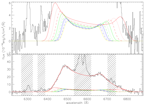
Figure 1: Example for the ten lines coming from the ten rings of the disk-like BLR of 3C390.3. Top panel shows the clear profiles of the ten lines from the ten rings, different colors and line styles represent lines from different rings. Color of red, green, blue, yellow, and line style of solid line, dotted line and dashed line show the line from the ring with increasing radius. Bottom panel shows the sum of the ten lines (thick solid line in red color), which further represents the best fitted results for the observed double-peaked H$\alpha$ around JD-2449870. Moreover, the shadow areas in the bottom panel show the masked regions for the narrow lines.

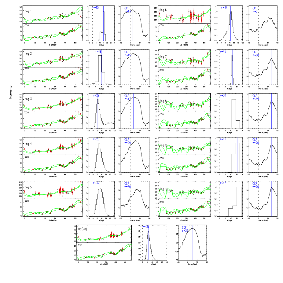
Figure 2: The results based on the SPEAR method and the CCF method applied to the light curves of the continuum emission and the ten lines from the ten rings. For each line and continuum, there are four panels, two panels show the light curves of the line and the continuum (red dots with error bars) and the the best descriptions for the light curves by the SPEAR method (green lines), one panel shows the distributions of the expected time lags between the line from the $i$th ring of BLR and the continuum through the SPEAR method (the distributions is normalized to have a maximum value equal to the peak value), and one panel shows the CCF results for the two light curves. The bottom panel shows the corresponding results for the continuum emission and the total observed broad H$\alpha$. In the figure, the vertical dotted lines show the positions with zero time lags, the blue solid lines show the peak positions of the distributions of the time lags through the SPEAR method, and the peak positions of the CCF results. The digital numbers in blue color gives the corresponding time lags. In the panels for the light curves, the unit for the continuum is ${\rm 10^{-15}{\rm erg/s/cm^{2}/\AA}}$, and the unit for the emission lines is ${\rm 10^{-12}{\rm erg/s/cm^{2}}}$

There are three steps being applied to complete the flux calibration for the line intensities of the ten lines from the ten rings. First and foremost, because the 67 spectra of 3C390.3 around 1995 are observed by different instruments in different observatories under different configurations, the measured line intensity based on the observed line profile should have low confidence level. Therefore, we collected the reliable values ($F_{AGN}$ with corresponding uncertainties) listed in the AGNWATCH project, with the completed flux calibration having been applied (Dietrich et al. 1998) for the observed lines. Besides, the line intensities in the AGNWATCH project include contributions from the narrow lines around H$\alpha$. In order to ignore the effects of narrow lines on the following determined time lags, the intensities of the narrow lines should be subtracted from $F_{AGN}$. Here, based on the intensity of [OIII]$\lambda 5007\AA$ in Dietrich et al. (1998) and the flux ratio of [NII] doublet and narrow H$\alpha$ to [OIII] in Dietrich et al. (2012), the total intensity of narrow lines around H$\alpha$ is determined as

$$\begin{split}&F_{narrow}=flux(H\alpha_{n})+flux([NII])\\ &\sim(3.53+1.34+0.44)\times flux([OIII])\\ &\sim 117\times 10^{-15}{\rm erg/s/cm^{2}}\end{split}$$ (1)

Finally, the available line intensities ($Flux_{i}(i=1,2,3,..,10)$) of the ten lines from the ten rings for each observed broad H$\alpha$ can be determined by the intensities ($flux_{i}$) from the direct observed lines without flux calibration,

$$Flux_{i}=\frac{flux_{i}}{\sum flux_{i}}\times(F_{AGN}-F_{narrow})$$ (2)

And, the uncertainty of $Flux_{i}$ can be determined by the uncertainties of $F_{AGN}$ and $flux([OIII])$. Then, the light curves of the continuum and the ten lines from the ten rings can be determined and shown in Figure 2. Here, the light curve of the continuum is the well-time binned one from the AGNWATCH Project (http://www.astronomy.ohio-state.edu/~agnwatch/3c390/lcv/).

Now, based on the light curves, we can check the dependence of the time lags for the ten lines on the radii of the ten rings. There are several commonly accepted CCF (Cross Correlation Function) methods to estimate time lag between two data series, such as the ZDCF method (Z-transfer Discrete Correlation Function, Edelson & Krolik 1988, Peterson 1993, White & Peterson 1994), the ICCF method (Interpolated Cross Correlation Function, Gaskell & Peterson 1987, Peterson 1993), the MCCF method (Modified Cross Correlation Function, Koratkar & Gaskell 1989, Koptelova et al. 2006) etc.. More recently, Zu et al. (2011) have reported one new method to estimate time lag between continuum and emission line of AGN (SPEAR method, Stochastic Process Estimation for AGN Reverberation), based on the assumption that all emission-line light curves are time-delayed, scaled, smoothed, and displaced versions of the continuum. This alternative approach fits the light curves directly using a damped random walk model (DRW model, Kelly et al. 2009, Kozlowski et al. 2010, MacLeod et al. 2010) and aligns them to recover the time lag and its statistical confidence limits. In the letter, both the ICCF method and the Zu’s SPEAR method are applied to estimate the time lags between the continuum emission and the ten lines from the rings.

When the ICCF method is applied, in order to ignore the effects of the large time gaps of the light curve as far as possible, only the data points within JD from JD-2449700 to JD-2450000 (around 300days) are considered. Then the corresponding uncertainty of the time lag can be determined by the Monte Carlo method as what we have done in Zhang et al. (2011b). When the SPEAR method is applied, in order to obtain good enough results about the light curves through the DRW method, all the data points in the light curves are considered. Here, we do not describe the SPEAR method in detail, which can be found in Zu et al. (2011) and in the website: https://bitbucket.org/nye17/javelin. When the SPEAR method is applied, the number of walkers, burn-in iterations and sampling iterations for each walker are 300, 300 and 300 respectively in the MCMC (Markov chain Monte Carlo method) analysis. Moreover, when the SPEAR method is applied, range from -10days to 100days is set as the boundaries for the time lag. The final results based on the ICCF method and the SPEAR method are shown in Figure 2.

Based on the results shown in Figure 2 (especially the distributions of the time lags through the SPEAR method, and the CCF results), the time lags between the continuum emission and the ten lines from the ten rings are increasing with encreasing the radii of the rings. More clearer results are shown in Figure 3. In Figure 3, we show the correlations between the flux weighted radii of the ten rings (in unit of ${\rm R_{G}}$) and the time lags determined by the SPEAR method and the CCF method. Here, the flux weighted radii of the ten rings with lower and higher boundaries are calculated through the standard elliptical accretion disk model. For the $i$th ($i=1,2,3...10$) ring, there are 67 flux weighted radii based on the lower and higher boundaries for the 67 rings of the 67 observed broad H$\alpha$. Then, the mean value is accepted as the flux weighted radius of the $i$th ring, and the corresponding uncertainty is estimated as the value of the flux weight radius of the $i$th ring minus the minimum inner boundary for the 67 $i$th rings of the 67 observed spectra. It is clear that there are well consistent time lags determined by the SPEAR method and by the CCF method. Moreover, we can find the time lags between the ten lines and the continuum emission are strongly linearly correlated with the radii of the ten rings,

$$\begin{split}\frac{R}{R_{G}}&=(19.45\pm 2.15)\times\frac{\tau_{SPEAR}}{\rm light-days}\\ &=(16.87\pm 1.91\times\frac{\tau_{CCF}}{\rm light-days}\end{split}$$ (3)

where $R$ means the flux weighted radii of the ten rings in unit of $R_{G}$. The corresponding values of Chi-square divided by number of degrees of freedom are 0.04 and 0.4 for results about $\tau_{SPEAR}$ and $\tau_{CCF}$. The results above are strongly support the accretion disk model for 3C390.3.

3 Discussions and Conclusions

Figure 3: On the correlation between the time lags determined by the SPEAR method and by the CCF method (left panel), and the correlation between the time lags and the radii of the rings (right panel). In the left panel, the sold circle represents the values for the total observed H$\alpha$. In the right panel, circles are for the time lags based on the SPEAR method, triangles are for values based on the CCF method, solid circle and solid triangle are for the total observed H$\alpha$. In the left panel, the solid line represents $\tau_{CCF}=\tau_{SPEAR}$. In the right panel, the solid line and the dotted line are the best fitted results (Equation 3) for the correlation about $\tau_{SPEAR}$ and for the correlation about $\tau_{CCF}$.

Before further discussion, we firstly check whether our results about the time lags are reliable, especially for the time lag between the total observed broad H$\alpha$ and the continuum emission. In Zu et al. (2011), the time lag between the continuum emission and the H$\beta$ determined by the SPEAR method is about $27.9^{+2.4}_{-1.5}$ light-days for 3C390.3, which is well consistent with our result of $\sim 25\pm 5$ light-days between the continuum emission and the observed H$\alpha$ by the SPEAR method. Moreover, the time lag between the continuum and the observed H$\alpha$ is about $20\pm 9$ light-days by the CCF method in Dietrich et al. (1998), which is consistent with our result $27\pm 5$ light-days by the CCF method. The consistencies above indicate our procedures to estimate the time lags by the SPEAR method and by the CCF method are reliable. And therefore, the results shown in Figure 2 and in Figure 3 have high confidence levels. In other words, the strong positive correlation shown in Figure 3 are reliable, which strongly support the accretion disk model for 3C390.3.

Besides to provide strong evidence for the accretion disk model for 3C390.3, the strong positive linear correlation shown in Figure 3 could provide one another way to independently estimate the black hole masses of 3C390.3,

$$\frac{M_{BH}}{10^{8}{\rm M_{\odot}}}=\frac{1.}{0.005687\times\frac{R}{R_{G}}/\frac{\tau}{\rm light-days}}$$ (4)

where the factor of ’0.005687’ is the value used to transfer the unit of ${\rm R_{G}}$ to the physical unit of light-days. Then, based on the Equation 3, the black hole masses of 3C390.3 are around $9.3^{+0.9}_{-1.1}\times 10^{8}{\rm M_{\odot}}$ if $R\propto\tau_{SPEAR}$ being considered, and the black hole masses are around $10.4^{+1.3}_{-1.1}\times 10^{8}{\rm M_{\odot}}$ if $R\propto\tau_{CCF}$ being considered. The black hole masses are very well consistent with the more recent result in Dietrich et al. (2012): $M_{BH}\sim 10^{9}{\rm M_{\odot}}$. The results not only indicate our results in Figure 3 are reliable, but also provide one optional independent method to determine black hole masses for double-peaked AGN besides the M-sigma method (Ferrarese & Merritt 2001, Gebhardt et al. 2000, Gültekin et al. 2009, Lewis & Eracleous 2006) and the Virialization method (Dietrich et al. 2012, Peterson et al. 2004, Woo et al. 2010).

Finally, we give our summary as follows. The time lags between the ten lines coming from the well split ten rings of the disk-like BLR and the continuum emission have been calculated through the SPEAR method and the CCF method, under the theoretical accretion disk model. Then, we can find one strong correlation between the time lags and the radii of the rings. Moreover, based on the correlation, the independently determined black hole masses of 3C390.3 are well consistent with the more recent values in the literature. The results above give further and strong evidence for the accretion disk model for 3C390.3.

References

- [\citeauthoryearBegelman et al.1980] Begelman M. C., Blandford R. D. & Rees M. J., 1980, Nature, 287, 307
- [\citeauthoryearBlandford & Mckee1982] Blandford R. D. & Mckee C. F., 1982, ApJ, 255, 419
- [\citeauthoryearBoroson & Laue2009] Boroson T. A. & Lauer T. R., 2009, Nature, 458, 53
- [\citeauthoryearBurbidge & Burbidge1971] Burbidge E. M. & Burbidge G. R., 1971, ApJ, 163, L21
- [\citeauthoryearChen & Halpern1989] Chen K. Y. & Halpern J. P., 1989, ApJ, 344, 115
- [\citeauthoryearDietrich et al.1998] Dietrich M., Peterson B. M., Albrecht P., Altmann M., Barth A. J., et al., 1998, ApJS, 115, 185
- [\citeauthoryearDietrich et al.2012] Dietrich M., Peterson B. M., Grier C. J., Bentz M .C., Eastman J., et al., 2012, ApJ, 757, 53D
- [\citeauthoryearEdelson & Krolik1988] Edelson R. A. & Krolik J. H., 1988, ApJ, 333, 646
- [\citeauthoryearEracleous & Halpern1994] Eracleous M. & Halpern J. P., 1994, ApJS, 90, 1
- [\citeauthoryearEracleous et al.1995] Eracleous M., Livio M., Halpern J. P., Storchi-Bergmann T., 1995, ApJ, 438, 610
- [\citeauthoryearEracleous et al.1997] Eracleous M., Halpern J. P., Gilbert A. M., Newman J. A., Filippenko A. V., 1997, ApJ, 490, 216
- [\citeauthoryearEracleous & Halpern2003] Eracleous M. & Halpern J. P., 2003, ApJ, 599, 886
- [\citeauthoryearFerrarese & Merritt2001] Ferrarese L. & Merritt D., 2001, MNRAS, 320, L30
- [\citeauthoryearFlohic & Eracleous2008] Flohic H. M. L. G. & Eracleous M., 2008, ApJ, 686, 138
- [\citeauthoryearGaskell & Peterson1987] Gaskell C. M. & Peterson B. ., 1987, ApJS, 65, 1
- [\citeauthoryearGaskell1996] Gaskell M., 1996, ApJ, 464, 107
- [\citeauthoryearGebhardt et al.2000] Gebhardt K., Bender R., Bower G., Dressler A., Faber S. M., et al., 2000, ApJ, 439, L13
- [\citeauthoryearGezari et al.2007] Gezari S., Halpern J. P., Eracleous M., 2007, ApJ, 169, 167
- [\citeauthoryearGliozzi et al.2006] Gliozzi M., Papadakis I. E., Rath C., 2006, A&A, 449, 969
- [\citeauthoryearGliozzi et al.2011] Gliozzi M., Titarchuk L., Satyapal S., Price D., Jang I., 2011, ApJ, 735, 16
- [\citeauthoryearGültekin et al.2009] Gültekin K., Richstone D. O., Gebhardt K., Lauer T. R., Tremaine S., et al., 2009, ApJ, 698, 198
- [\citeauthoryearHorne et al.2004] Horne K., Peterson B. M., Collier S. J., Netzer H. 2004, PASP, 116, 465
- [\citeauthoryearKelly et al.2009] Kelly B. C., Bechtold J., Siemiginowska A. 2009, ApJ, 698, 895
- [\citeauthoryearKollatschny & Zetzl12011] Kollatschny W. & Zetzl1 M., 2011, Nature, 470, 366
- [\citeauthoryearKoratkar & Gaskell1989] Koratkar A. P. & Gaskell C. M., 1989, ApJ, 345, 637
- [\citeauthoryearKoptelova et al.2006] Koptelova E. A., Oknyanskij V. L., Shimanovskaya E. W., 2006, A&A, 452, 37
- [\citeauthoryearKozlowski et al.2010] Kozlowski S., Kochanek C. S., Udalski A., Wyrzykowski L., Soszynski I., et al., 2010, ApJ, 708, 927
- [Leighly et al., 1997] Leighly K. M., O’Brien P. T., Edelson R., George I. M., Malkan M. A., Matsuoka M., Mushotzky R. F., Peterson B. M., 1997, ApJ, 483, 767
- [Lewis & Eracleous, 2006] Lewis K. T. & Eracleous M., 2006, ApJ, 642, 711
- [\citeauthoryearLivio & Xu1997] Livio M. & Xu C., 1997, ApJ, 478, L63
- [\citeauthoryearMacLeod et al.2010] MacLeod C. L., Ivezic Z., Kochanek C. S., KozLowski S., Kelly B., et al., 2010, ApJ, 721, 1014
- [\citeauthoryearNetzer1982] Netzer H., 1982, MNRAS, 198, 589
- [O’Brien et al., 1998] O’Brien P.T., Dietrich M., Leighly K., Alloin D., Clavel J., et al., 1998, ApJ, 509, 163
- [\citeauthoryearPerez et al.1988] Perez E., Penston M. V., Tadhunter C., Mediavilla E., Moles M., 1988, MNRAS, 230, 353
- [\citeauthoryearPeterson1993] Peterson, B. M., 1993, PASP, 105, 247
- [\citeauthoryearPeterson et al.2004] Peterson B. M., Ferrarese L., Gilbert K. M., Kaspi, S., Malkan M. A., et al., 2004, ApJ, 613, 682
- [\citeauthoryearPopovic et al.2011] Popovic L. C., Shapovalova A. I., Ilic D., Kovacevic A., Kollatschny W., Burenkov A. N., Chavushyan V. H., Bochkarev N. G., Leon-Tavares J., 2011, A&A, 528, 130
- [\citeauthoryearSambruna et al.2009] Sambruna R. M., Reeves J. N., Braito V., Lewis K. T., Eracleous M., et al., 2009, ApJ, 700, 1473
- [\citeauthoryearSergeev et al.2002] Sergeev S. G., Pronik V. I., Peterson B. M., Sergeeva E. A., Zheng W., 2002, ApJ, 576, 660
- [\citeauthoryearSergeev et al.2011] Sergeev S. G., Kilmanov S. A., Doroshenko V. T., Efimov Y. S., Nazarov S. V., Pronik V. I., 2011, MNRAS, 410, 1877
- [\citeauthoryearShapovalova et al.2001] Shapovalova A. I., Burenkov A. N., Carrasco L., Chavushyan V. H., Doroshenko V. T., et al., 2001, A&A, 376, 775
- [\citeauthoryearShapovalova et al.2010] Shapovalova A. I., Popovic L. C., Burenkov A. N., Chavushyan V. H., Ilic D., et al., 2010, A&A, 517, 42
- [\citeauthoryearVeilleux & Zheng1991] Veilleux S. & Zheng W., 1991, ApJ, 377, 89
- [\citeauthoryearWhite & Peterson1994] White R. J. & Peterson B. M., 1994, PASP, 106, 876
- [\citeauthoryearWoo et al.2010] Woo J. H. Treu T., Barth A. J., Wright S. A., Walsh J. L., et al., 2010, ApJ, 716, 269
- [\citeauthoryearZhang et al.2007] Zhang X. G., Dultzin D., Wang T. G., 2007, MNRAS, 377, 1215
- [\citeauthoryearZhang2011a] Zhang X. G., 2011a, MNRAS, 416, 2857, Paper I
- [\citeauthoryearZhang2011b] Zhang X. G., 2011b, ApJ, 741, 104
- [\citeauthoryearZhang2012] Zhang X. G., 2013, MNRAS, 429, 2274, arXiv:1211.6204, Paper II
- [\citeauthoryearZheng1996] Zheng W., 1996, AJ, 111, 1498
- [\citeauthoryearZu et al.2011] Zu Y., Kochanek C. S., Peterson B. M., 2011, ApJ, 735, 80