Effect of anisotropic band curvature on carrier multiplication in graphene

Abstract

We study relaxation of an excited electron in the conduction band of intrinsic graphene at zero temperature due to production of interband electron-hole pairs by Coulomb interaction. The electronic band curvature, being anisotropic because of trigonal warping, is shown to suppress relaxation for a range of directions of the initial electron momentum. For other directions, relaxation is allowed only if the curvature exceeds a finite critical value; otherwise, a nondecaying quasiparticle state is found to exist.

I Introducton

Carrier multiplication is a process in which a single photon, absorbed by a material, produces several electron-hole (e-h) pairs. Typically, this happens when the primary photoexcited e-h pair produces a number of secondary pairs of smaller energy via electron-electron collisions. This process is very important for optoelectronic applications: the more e-h pairs are produced by a single photon, the more efficiently one can convert light into electric current. Graphene is an obvious candidate for efficient carrier multiplication, since (i) it has wide electronic bands and no energy gap, and (ii) electron-electron scattering can be much faster than electron-phonon scattering. Indeed, the dynamics of photoexcited carriers in graphene has become a subject of many studies, both theoretical and experimental.Rana2007 ; George2008 ; Dawlaty2008 ; Sun2008 ; Bao2009 ; Kumar2009 ; Newson2009 ; Plochocka2009 ; Lui2010 ; Winzer2010 ; Hale2011 ; Winnerl2011 ; Breusing2011 ; Kim2011 ; Strait2011 ; Li2012 ; Winzer2012 ; Song2012 ; Brida2012 ; Tielrooj2012 ; Winzer2013 ; Winnerl2013 ; SunWu2013

In spite of the numerous studies, this dynamics is still not fully understood. Notably, the most basic issue, that of the role of electron-electron collisions in the relaxation of a single photoexcited carrier in the intrinsic graphene, is still under debate. It is well known (see, e. g., Ref. LL9, ) that due to simultaneous energy and momentum conservation, decay of quasiparticles is allowed or forbidden, depending on the curvature of the quasiparticle spectrum. In the context of graphene, the Dirac spectrum is linear, so it is exactly on the borderline between the two cases.Gonzalez1996 Indeed, if an electron in the conduction band with momentum ${\rm\bf p}$ and energy $v|{\rm\bf p}|$ ($v$ being the Dirac velocity) is scattered into the state with another momentum ${\rm\bf p}^{\prime}$ and lower energy $v|{\rm\bf p}^{\prime}|<v|{\rm\bf p}|$, creating a hole in the valence band with momentum ${\rm\bf p}_{h}$ and another electron in the conduction band with momentum ${\rm\bf p}_{e}$, the momentum and energy conservation conditions,

$${\rm\bf p}={\rm\bf p}^{\prime}+{\rm\bf p}_{e}+{\rm\bf p}_{h},$$ (1a)

$$v|{\rm\bf p}|=v|{\rm\bf p}^{\prime}|+v|{\rm\bf p}_{e}|+v|{\rm\bf p}_{h}|,$$ (1b)

are compatible only in the special case when all vectors lie on the same line. Different ways to resolve the uncertainty have been advocated.Rana2007 ; Li2012 ; Brida2012 ; Winzer2013 ; Fritz2008 ; Foster2009 ; Basko2009 ; Golub2011 Note that the collision process in question is precisely the one responsible for carrier multiplication (Fig. 1).

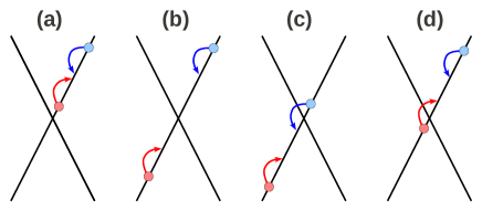
Figure 1: Various collision processes for an excited electron in the conduction band. The straight lines represent the Dirac cones and the circles represent electrons. Processes (a), (b) conserve the number of carriers in the conduction and valence bands separately. Processes (a)–(c) are forbidden by the Pauli principle in the intrinsic graphene at zero temperature. Process (d) corresponds to carrier multiplication (the initial electron produces one more electron and one hole).

It might seem that importance of the above-mentioned problem of a single excited carrier is limited to low photoexcitation intensities. However, if many e-h pairs are created under intense photoexcitation, it is important to know whether the population equilibration between the valence and the conduction band happens as quickly as the thermalization within each band. For example, only if the interband population relaxation is slow enough, a population inversion between the bands can be achieved, and one can think about lasing. Among various two-electron collision processes, shown in Fig. 1, only the processes (d) (carrier multiplication) and (c) (Auger recombination, reciprocal to the multiplication) can transfer electrons between the bands. If these are suppressed, three-particle collisions are required to equilibrate the populations of the conduction and the valence bands.

In the present work, we study relaxation of an excited electron in the conduction band of intrinsic graphene at zero temperature due to electron-electron collisions (the process (d) in Fig. 1), going beyond the Dirac approximation and taking into account the electronic band curvature. Because the curvature is anisotropic due to the trigonal warping, the result turns out to depend on the direction of the initial electron momentum, as was also noted in Ref. Golub2011, . For a certain range of directions, the process is forbidden. For the directions when relaxation is allowed, we calculate its rate.

If the curvature is weak, the problem corresponds to that of a discrete state coupled to a continuum whose density of states is abruptly cut off precisely at the energy of the discrete level, which can be viewed as a special case of the Fano problem.Fano Indeed, in the sector with the fixed total momentum ${\rm\bf p}$, the single-particle excitation is a discrete level with the energy $vp$. The three-particle density of states vanishes below this energy, and exhibits a steplike discontinuity at the energy $vp$. In this situation, the presumable decay of the discrete state into the continuum cannot be described by the Fermi golden rule, since the latter is valid only when the density of states in the continuum is a smooth function of energy at the position of the discrete level. Below it is shown that the quantum-mechanical level repulsion between the discrete state and the continuum plays a major role in this problem. As a result, a nondecaying quasiparticle state exists (that is, its lifetime being determined by mechanisms other that electron-electron interaction). Still, the quasiparticle spectral weight is reduced, some part of it being transferred to the continuum of the multiparticle excitations. The quasiparticle state can relax by producing electron-hole pairs only when the band curvature along the allowed directions exceeds a finite critical value, needed to overcome the level repulsion.

II Calculation

To derive the results, outlined above, let us describe the electrons by a two-component column fermionic field operator $\hat{\psi}_{\alpha}({\rm\bf r})$, where $\alpha=1,\ldots,N$ labels electronic species (the valley and spin degeneracy in graphene correspond to $N=4$). The Hamiltonian is given by

$$\begin{split}\hat{H}={}&{}\sum_{\alpha=1}^{N}\int\hat{\psi}_{\alpha}^{\dagger}({\rm\bf r})\,h(-i\boldsymbol{\nabla})\,\hat{\psi}_{\alpha}({\rm\bf r})\,d^{2}{\rm\bf r}+{}\\ {}&{}+\frac{e^{2}}{2}\int\frac{\hat{\rho}({\rm\bf r})\,\hat{\rho}({\rm\bf r}^{\prime})}{|{\rm\bf r}-{\rm\bf r}^{\prime}|}\,d^{2}{\rm\bf r}\,d^{2}{\rm\bf r}^{\prime}.\end{split}$$ (2)

The first term in Eq. (2) represents the kinetic energy of electrons, described by the single-particle Hamiltonian,

$$h({\rm\bf p})=v(p_{x}\sigma_{x}+p_{y}\sigma_{y})-\zeta_{3}[(p_{x}^{2}-p_{y}^{2})\sigma_{x}-2p_{x}p_{y}\sigma_{y}]-\zeta_{0}p^{2},$$ (3)

$\sigma_{x},\sigma_{y}$ being the Pauli matrices. It determines the single-particle dispersion relation to $O(p^{2})$, which we write as

$$\epsilon_{\rm\bf p}^{e,h}=vp\mp\zeta_{0}p^{2}\mp\zeta_{3}p^{2}\cos{3}\varphi\equiv{v}p\pm\zeta_{\varphi}{p}^{2},$$ (4)

where $\epsilon^{e}_{\rm\bf p}(\epsilon^{h}_{\rm\bf p})$ is the energy of an electron in the conduction band (a hole in the valence band) with momentum ${\rm\bf p}$, and $\varphi$ is the polar angle of ${\rm\bf p}$. The coefficients can be estimated from the tight-binding modelGruneis2008 : the Dirac velocity $v\approx{7}\>\mbox{eV}\cdot\mbox{\AA}$, the trigonal warping coefficient $\zeta_{3}\approx{5}\>\mbox{eV}\cdot\mbox{\AA}^{2}$, and the electron-hole asymmetry $\zeta_{0}\approx{0}.8\>\mbox{eV}\cdot\mbox{\AA}^{2}$. Neglecting the terms proportional to $\zeta_{0},\zeta_{3}$ in Eq. (3) corresponds to the Dirac approximation $h({\rm\bf p})=v{\rm\bf p}\cdot\boldsymbol{\sigma}$.

The last term in Eq. (2) describes Coulomb interaction between the electrons, with the electronic density

$$\hat{\rho}({\rm\bf r})=\sum_{\alpha=1}^{N}\hat{\psi}_{\alpha}^{\dagger}({\rm\bf r})\hat{\psi}_{\alpha}({\rm\bf r}),$$ (5)

and the background dielectric constant $\varepsilon_{b}$ of the substrate incorporated into $e^{2}$. The dimensionless Coulomb coupling strength $e^{2}/v$ can be small if $\varepsilon_{b}$ is large enough. The largest value of $e^{2}/v\approx{2}.2$ is attained for a graphene sheet suspended in vacuum, $\varepsilon_{b}=1$ .

The quasiparticle decay rate is given by $-2\Sigma_{\rm\bf p}(\epsilon)$, where $\Sigma_{\rm\bf p}(\epsilon)$, the retarded self-energy projected on the eigenstate of the single-particle Hamiltonian with momentum ${\rm\bf p}$, should be taken at $\epsilon$ corresponding to the quasiparticle pole of the Green’s function. In the first approximation, it can be taken on the mass shell, $\epsilon=\epsilon^{e}_{\rm\bf p}$ or $\epsilon=-\epsilon^{h}_{-{\rm\bf p}}$. The lowest order of the perturbation theory in the Coulomb interaction, which contributes to $\mathop{\mathrm{Im}}\nolimits\Sigma_{\rm\bf p}(\epsilon)$, is the second one. It describes decay of the one-particle state (an electron or a hole) into three-particle excitations (an electron or a hole plus an e-h pair). It turns out, however, that in the Dirac approximation, the second-order $\mathop{\mathrm{Im}}\nolimits\Sigma_{\rm\bf p}(\epsilon)$ has a steplike discontinuity on the mass shell, invalidating the simple Fermi golden rule recipe for calculating the decay rate.Gonzalez1996 Explicitly, at $|\epsilon-vp|\ll{vp}$,

$$\mathop{\mathrm{Im}}\nolimits\Sigma_{\rm\bf p}(\epsilon)=-\gamma_{\rm\bf p}\,\theta(\epsilon-vp),$$ (6a)

$$\gamma_{\rm\bf p}=\pi\left(\frac{N}{24}-\ln\frac{2}{e^{2/3}}\right)\left(\frac{e^{2}}{v}\right)^{2}vp,$$ (6b)

$\theta(x)$ being the step function. In Eq. (6b), $N/24$ comes from the bubble diagram (the direct term), while $\ln(2/e^{2/3})$ comes from the exchange diagram (see Appendix A.2 for details). At $N=4$, the exchange term is more than six times smaller than the direct term.

One may consider higher orders of the perturbation theory in $e^{2}/v$, while remaining within the Dirac approximation. Decay into $(2n+1)$-particle excitations, which involves three-particle excitations as virtual intermediate states, is suppressed by energy and momentum conservation as $\propto(\epsilon-vp)^{n}\theta(\epsilon-vp)$ (see Appendix A.2), so inclusion of many-particle excitations does not help to resolve the uncertainty. Dressing the decay into three-particle states by higher-order corrections can be performed by treating $1/N$ as a formal small parameter. This selects the random-phase-approximation (RPA) sequence as the dominant subclass of diagrams. In RPA, $\mathop{\mathrm{Im}}\nolimits\Sigma_{\rm\bf p}(\epsilon=vp)$ strictly vanishesGonzalez1996 ; Khveshchenko2006 ; DasSarma2007 . Explicitly (see Appendix A.6),

$$\mathop{\mathrm{Im}}\nolimits\Sigma_{\rm\bf p}(\epsilon)=-\frac{4(\epsilon-vp)}{\pi{N}}\,\theta(\epsilon-vp)\ln\frac{\xi_{\mathrm{RPA}}}{\epsilon-vp},$$ (7)

where the upper cutoff of the logarithm is $\xi_{\mathrm{RPA}}=\min\{vp,(Ne^{2}/v)^{2}vp\}$, and Eq. (7) is valid at $\epsilon-vp\ll\xi_{\mathrm{RPA}}$. If $Ne^{2}/v\ll{1}$, the perturbative expression of Eqs. (6a), (6b) is still valid in the parametric region of energies $(Ne^{2}/v)^{2}vp\ll\epsilon-vp\ll{vp}$, while for $Ne^{2}/v\gtrsim{1}$ Eqs. (6a), (6b) are never valid, and only Eq. (7) holds.

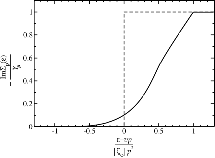
Figure 2: Smearing of the steplike discontinuity in the second-order self-energy for $\zeta_{\varphi}>0$ at $N=4$. The dashed and solid curves represent $-\mathop{\mathrm{Im}}\nolimits\Sigma_{\rm\bf p}(\epsilon)$ in and beyond the Dirac approximation, respectively. For $\zeta_{\varphi}<0$ the curve should be rotated by $180^{\circ}$.

Beyond the Dirac approximation, we take into account the terms proportional to $p^{2}$ in Eq. (3). Assuming them to be small compared to the main Dirac term $vp$, we neglect them wherever they produce small corrections to regular expressions (e. g., corrections to the eigenstates of the single-particle Hamiltonian), and take them into account only in those terms which are singular at $\epsilon\to{vp}$. In the second order of the perturbation theory, instead of Eq. (6a), we obtain (see Appendix A.3 for details of the calculation)

$$\begin{split}\zeta_{\varphi}>0:&\quad\mathop{\mathrm{Im}}\nolimits\Sigma_{\rm\bf p}(\epsilon)=-\gamma_{\rm\bf p}\,\mathcal{F}_{N}\!\left(\frac{\epsilon-vp}{\zeta_{\varphi}{p}^{2}}\right),\\ \zeta_{\varphi}<0:&\quad\mathop{\mathrm{Im}}\nolimits\Sigma_{\rm\bf p}(\epsilon)=-\gamma_{\rm\bf p}\left[1-\mathcal{F}_{N}\!\left(-\frac{\epsilon-vp}{|\zeta_{\varphi}|p^{2}}\right)\right],\end{split}$$ (8)

where the function $\mathcal{F}_{N}(z)$ is defined in Appendix A.3. The result of its numerical evaluation for $N=4$ is plotted in Fig. 2. $\mathcal{F}_{N}(z)=0$ for $z<-1$ . On the mass shell, $\epsilon=vp+\zeta_{\varphi}{p}^{2}$, $\mathcal{F}_{N}=1$. So, electronic relaxation is allowed if $\cos{3}\varphi<-\zeta_{3}/\zeta_{0}\approx{0}.16$, with the rate $2\gamma_{\rm\bf p}$, and forbidden for $\cos{3}\varphi>-\zeta_{3}/\zeta_{0}$. For a hole in the valence band with momentum ${\rm\bf p}$, the conditions are just the opposite.

Just like Eq. (6a), Eq. (8) is valid for $(Ne^{2}/v)^{2}vp\ll\epsilon-vp\ll{vp}$. When $|\zeta_{\varphi}|p^{2}\lesssim(Ne^{2}/v)^{2}vp$ and $N\gg{1}$, the self-energy should be calculated from RPA in the presence of the $p^{2}$ terms. For this, one first has to calculate the polarization operator $\Pi_{\rm\bf q}(\omega)$ (the effect of non-Dirac dispersion on the polarization operator in graphene was also studied in Refs. Stauber2010, ; Stauber2011, ). Here we take the $p^{2}$ terms into account only near the singularity at $\omega\to{v}q$, which becomes smeared as (see Appendix A.5 for details of the calculation)

$$\Pi_{\rm\bf q}(\omega\approx{vq})=-\frac{Nq^{2}}{16\sqrt{2vq}}\,\frac{1}{\sqrt{|\zeta_{\varphi}|q^{2}}}\,\mathcal{P}\!\left(\frac{\omega-vq}{|\zeta_{\varphi}|q^{2}}\right),$$ (9a)

$$\mathcal{P}(z)=\frac{8\sqrt{1-z}}{3\pi}\left[(1+z)\,K\!\left(\frac{2}{1-z}\right)-z\,E\!\left(\frac{2}{1-z}\right)\right],$$

(9b)

where $E(m)$ and $K(m)$ are the complete elliptic integrals. The function $\mathcal{P}(z)$ is plotted in Fig. 3. Finally, $\mathop{\mathrm{Im}}\nolimits\Sigma_{\rm\bf p}(\epsilon)$ is evaluated in Appendix A.7. It vanishes for $\epsilon\leq{v}p-|\zeta_{\varphi}|p^{2}$. We give its explicit value on the mass shell only, which has a compact form:

$$\mathop{\mathrm{Im}}\nolimits\Sigma_{\rm\bf p}(\epsilon^{e}_{\rm\bf p})=-\,\frac{64}{15\pi}\,\frac{\zeta_{\varphi}{p}^{2}}{N}\,\theta(\zeta_{\varphi}).$$ (10)

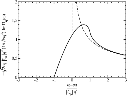
Figure 3: Smearing of the square root singularity at $\omega\to{vq}$ in the imaginary part of the polarization operator, $-\mathop{\mathrm{Im}}\nolimits\Pi_{\rm\bf q}(\omega)$. The dashed curve represents the Dirac approximation which gives $1/\sqrt{z}$, the solid curve represents the function $\mathop{\mathrm{Im}}\nolimits\mathcal{P}(z)$, defined in Eq. (9b).

The above results [Eqs. (8) and (10)] correspond to the Fermi golden gule (FGR) with lowest-order or RPA-dressed transition matrix elements. They are valid in the case $|\zeta_{\varphi}|p^{2}\gg\min\{\gamma_{\rm\bf p},vp/N\}$, when the singularity in $\mathop{\mathrm{Im}}\nolimits\Sigma_{\rm\bf p}(\epsilon)$ is strongly smeared by the band curvature. Let us study the opposite case, when the dominant energy scale is $\gamma_{\rm\bf p}$ itself, e. g., near the directions where $\zeta_{\varphi}=0$. It should be recalled that FGR works only when the density of the final states of the decay (three-particle excitations in the present case) is approximately constant, in which case the quasiparticle spectral peak has the Lorentzian shape. When the density of states is not smooth, FGR-based approachesRana2007 ; Winzer2010 ; Kim2011 ; Winzer2012 ; Winzer2013 are not valid, and the quasiparticle spectral peak is manifestly non-Lorentzian. To determine the quasiparticle properties in the non-FGR regime, let us study the single-particle (retarded) Green’s function $G_{\rm\bf p}(\epsilon)$, which determines the quasiparticle spectral function, $-(1/\pi)\mathop{\mathrm{Im}}\nolimits{G}_{\rm\bf p}(\epsilon)$.

Let us first analyze the most “dramatic” case when $\mathop{\mathrm{Im}}\nolimits\Sigma_{\rm\bf p}(\epsilon)$ is given by Eq. (6a). In this case, the retarded Green’s function (or, more precisely, its projection on the eigenstate of the single-particle Hamiltonian with momentum ${\rm\bf p}$) is given by

$$G_{\rm\bf p}(\epsilon)=\left[\epsilon-vp+\frac{\gamma_{\rm\bf p}}{\pi}\ln\frac{\xi_{\mathrm{max}}}{|\epsilon-vp|}+i\gamma_{\rm\bf p}\theta(\epsilon-vp)\right]^{-1},$$ (11)

with the real part of the self-energy reconstructed from the Kramers-Kronig relation, and $\xi_{\mathrm{max}}\sim{vp}$ determines the ultraviolet cutoff of the logarithmic divergence, since Eq. (6a) is valid for $\epsilon-vp\ll{vp}$ onlycutoff . $G_{\rm\bf p}(\epsilon)$ has a real pole at $\epsilon-vp=-\Delta_{\rm\bf p}<0$. Its existence immediately follows from the fact that $\mathop{\mathrm{Re}}\nolimits\Sigma_{\rm\bf p}(\epsilon)<0$, which, in turn, is a consequence of the usual quantum-mechanical level repulsion: the quasiparticle level is repelled from the three-particle continuum. Note that introduction of any infinitesimal broadening of the step function does not affect this result at all. The real pole corresponds to a quasiparticle state with an infinite lifetime. Even though the quasiparticle does not decay into the continuum, the latter still takes away part of the spectral weight, which manifests itself in the residue $Z_{\rm\bf p}<1$ at the pole. With logarithmic precision we can evaluate

$$\Delta_{\rm\bf p}=\frac{\gamma_{\rm\bf p}}{\pi}\ln\frac{\xi_{\mathrm{max}}}{\gamma_{\rm\bf p}},\quad Z_{\rm\bf p}=\frac{1}{1+1/\ln(\xi_{\mathrm{max}}/\gamma_{\rm\bf p})}.$$ (12)

(We remind that Eq. (11) is valid only when $\gamma_{\rm\bf p}/\xi_{\mathrm{max}}\sim{N}(e^{2}/v)^{2}\ll{1}$, so that the logarithm is large). The spectral function for $\xi_{\mathrm{max}}/\gamma_{\rm\bf p}=10$ is plotted in Fig. 4.

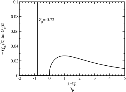
Figure 4: The quasiparticle spectral function (in the units of $\gamma_{\rm\bf p}$), as determined from Eq. (11) for $\xi_{\mathrm{max}}/\gamma_{\rm\bf p}=10$. The vertical peak represents the $\delta$-function with the spectral weight $Z_{\rm\bf p}\approx{0}.72$.

If now one gradually increases the band curvature $\zeta_{\varphi}{p}^{2}>0$, (i) the bare quasiparticle level is shifted to $\epsilon=vp+\zeta_{\varphi}{p}^{2}$, (ii) the spectral boundary of the continuum is shifted to $\epsilon=vp-\zeta_{\varphi}{p}^{2}$, and (iii) the logarithmic divergence in $\mathop{\mathrm{Re}}\nolimits\Sigma_{\rm\bf p}(\epsilon\to{vp})$ at $\epsilon\to{vp}$ is cut off at $\epsilon-vp\sim\zeta_{\varphi}{p}^{2}$. The dressed quasiparticle level enters the continuum at some critical value of $\zeta_{\varphi}{p}^{2}$, needed to overcome the level repulsion. This critical value can be determined from the condition $G_{\rm\bf p}^{-1}(vp+\zeta_{\varphi}{p}^{2})=0$, and with logarithmic precision, it is given by $\zeta_{\varphi}{p}^{2}=[\gamma_{\rm\bf p}/(2\pi)]\ln(\xi_{\mathrm{max}}/\gamma_{\rm\bf p})$. At this point the quasiparticle state acquires a finite decay rate, whose value for sufficiently large $\zeta_{\varphi}{p}^{2}$ is given by $-2\mathop{\mathrm{Im}}\nolimits\Sigma_{\rm\bf p}(\epsilon_{\rm\bf p}^{e})$, as determined by Eq. (8).

In RPA, suppression of $\mathop{\mathrm{Im}}\nolimits\Sigma_{\rm\bf p}(\epsilon)$, Eq. (7), at $\epsilon-vp\lesssim\xi_{\mathrm{RPA}}$ cuts off the logarithmic divergence in $\mathop{\mathrm{Re}}\nolimits\Sigma_{\rm\bf p}(\epsilon\to{vp})$ at $\epsilon-vp\sim\xi_{\mathrm{RPA}}$ [here $\xi_{\mathrm{RPA}}=\min\{vp,(Ne^{2}/v)^{2}vp\}$ is the same as in Eq. (7)]. Since $\xi_{\mathrm{RPA}}\gg\gamma_{\rm\bf p}$, we can take $\mathop{\mathrm{Re}}\nolimits\Sigma_{\rm\bf p}(\epsilon=vp)$ to find the quasiparticle pole,

$$\Delta_{\rm\bf p}\approx-\mathop{\mathrm{Re}}\nolimits\Sigma_{\rm\bf p}(\epsilon=vp)$$:

$$\Delta_{\rm\bf p}\approx\frac{\gamma_{\rm\bf p}}{\pi}\ln\frac{\xi_{\mathrm{max}}}{\xi_{\mathrm{RPA}}}\quad(Ne^{2}/v\ll{1}),$$ (13a)

$$\Delta_{\rm\bf p}\sim\frac{vp}{N}\quad(Ne^{2}/v\gg{1}),$$ (13b)

where $\xi_{\mathrm{max}}/\xi_{\mathrm{RPA}}\sim(Ne^{2}/v)^{-2}$. When $Ne^{2}/v\ll{1}$, the logarithm is large, so Eq. (13a) has logarithmic precision. When $Ne^{2}/v\gg{1}$, Eq. (13b) represents just an order-of-magnitude estimate obtained by plugging Eq. (7) into the Kramers-Kronig relation, and integrating from $\epsilon-vp=0$ to $\epsilon-vp\sim{vp}$. To find the residue at the pole, we note that at $0<vp-\epsilon\ll\xi_{\mathrm{RPA}}$, from Eq. (7) and the Kramers-Kronig relation one obtains

$$-\frac{\partial\Sigma_{\rm\bf p}(\epsilon)}{\partial\epsilon}\approx\frac{4}{\pi^{2}N}\int\limits_{0}^{\xi_{\mathrm{RPA}}}\frac{\xi\ln(\xi_{\mathrm{RPA}}/\xi)\,d\xi}{(\xi+vp-\epsilon)^{2}}\approx\frac{2}{\pi^{2}N}\ln^{2}\frac{\xi_{\mathrm{RPA}}}{vp-\epsilon},$$ (14)

which gives

$$Z_{\rm\bf p}=\left(1+\frac{2\ln^{2}N}{\pi^{2}N}\right)^{-1},$$ (15)

with logarithmic precision. The critical value of the band curvature, when the quasiparticle level enters the continuum and acquires a finite decay rate is given by $\zeta_{\varphi}{p}^{2}\approx\Delta_{\rm\bf p}/2$.

It is important that the existence of the infinitely narrow quasiparticle peak in the Dirac approximation, obtained above using the perturbation theory in $e^{2}/v$ and $1/N$ expansion, is, in fact, more general that these approximations. Indeed, the existence of the peak follows from two facts: (i) $\mathop{\mathrm{Im}}\nolimits\Sigma_{\rm\bf p}(\epsilon<vp)=0$, which holds in any order of the perturbation theory because of energy and momentum conservation as discussed in Appendix A.2, and (ii) $\mathop{\mathrm{Re}}\nolimits\Sigma_{\rm\bf p}(\epsilon\to{vp})<0$, which is a consequence of the level repulsion between the single-particle and the three-particle states. When the band curvature is included, the quasiparticle peak and the continuum are pushed towards each other for $\zeta_{\varphi}>0$, and away from each other for $\zeta_{\varphi}<0$. Consequently, the requirement for the band curvature to exceed a finite critical value in order to overcome the level repulsion and to produce quasiparticle decay, is also more general than the approximations used here. The calculation of critical value itself, of course, does rely on approximations.

Still, one cannot exclude the appearance of nonzero $\mathop{\mathrm{Im}}\nolimits\Sigma_{\rm\bf p}(\epsilon<vp)$ in the Dirac approximation due to nonperturbative effects. For example, nonperturbative generation of spectral weight in $\mathop{\mathrm{Im}}\nolimits\Pi_{\rm\bf q}(\omega)$ at $\omega<vq$ due to excitonic effects has been discussed in Ref. Mishchenko2008, , even though the validity of these results has been questioned in Ref. Sodemann2012, . This issue calls for further investigation.

III Discussion

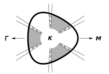
Figure 5: Directions of the electron momentum ${\rm\bf p}$ counted from the $K$ point for which a photoexcited e-h pair is subject to relaxation by production of interband e-h pairs (carrier multiplication). The thick solid curve represents the contour $\epsilon^{e}_{\rm\bf p}+\epsilon^{h}_{-{\rm\bf p}}=2\>\mbox{eV}$, as determined by Eq. (4). The gray area shows the directions of ${\rm\bf p}$ where both the electron with momentum ${\rm\bf p}$ and the hole with momentum $-{\rm\bf p}$ are subject to relaxation; along the directions in the hatched area, only the hole is subject to relaxation.

Let us discuss some experimental implications of the obtained results. In an optical experiment, the incident photon of the frequency $\omega$ produces an electron with momentum ${\rm\bf p}$ and a hole with momentum $-{\rm\bf p}$. Their energies satisfy $\epsilon^{e}_{\rm\bf p}+\epsilon^{h}_{-{\rm\bf p}}=\omega$, which constrains ${\rm\bf p}$ to a trigonally warped circle, shown in Fig. 5 for $\omega=2\>\mbox{eV}$. The direction of ${\rm\bf p}$ is determined by the photon polarization. If the excitation density is low, one can neglect intraband collisions between the photoexcited electrons and holes. According to the above results, when the band curvature is sufficiently large, the electron can relax by producing interband e-h pairs (carrier multiplication) if the direction of its momentum (the polar angle $\varphi$) satisfies $\zeta_{\varphi}=-\zeta_{3}\cos{3}\varphi-\zeta_{0}>0$ (shown in Fig. 5 by the gray area). The hole can relax if $-\zeta_{\pi-\varphi}=-\zeta_{3}\cos{3}\varphi+\zeta_{0}>0$ (gray and hatched areas on Fig. 5).

The discussed anisotropy of the electronic relaxation has some implications for the two-phonon Raman scattering, whose intensity is suppressed by electronic relaxation.Basko2008 ; Venezuela2011 . Namely, it favors the electronic states near the $KM$ direction (white sectors in Fig. 5, the states not subject to relaxation) to provide the dominant contribution to the two-phonon Raman intensity, as has been observed experimentally.Huang2010 ; Yoon2011 Another mechanism favoring the electronic states near the $KM$ direction is the anisotropy of the electron-phonon coupling.Venezuela2011 ; Narula2012

If the band curvature is too weak so that the quasiparticle state does not decay, its spectral weight $Z_{\rm\bf p}$ is still reduced, $Z_{\rm\bf p}<1$, since part of the spectral weight is transferred to three-particle excitations. It means that an initial excitation, produced by a short optical pulse, has a finite probability $1-Z_{\rm\bf p}$ to produce many-particle excitations, the typical time of the processes being $\sim{1}/\gamma_{\rm\bf p}$ (since $\gamma_{\rm\bf p}$ is the typical energy scale of the features in the spectral function). Thus, on average, the total number of e-h pairs per absorbed photon will exceed unity, so one can still speak about carrier multiplication even in the regime of weak band curvature.

IV Acknowledgements

The author is grateful to R. Asgari, I. V. Gornyi and M. Polini for stimulating discussions.

Appendix A Self-energy and polarization operator in the Dirac approximation and beyond

A.1 General remarks about the calculation

Figure 6: (a) The basic elements of the diagrammatic technique (the solid line represents the electronic Green’s function, the wavy line represents the Coulomb interaction) and the corresponding analytical expressions. (b) The two diagrams (direct and exchange) contributing to $\mathop{\mathrm{Im}}\nolimits\Sigma_{\rm\bf p}(\epsilon)$ in the second order in $e^{2}/v$. (c) Electronic polarization operator. (d) The RPA series for the self-energy.

The calculation is performed using the standard zero-temperature diagrammatic technique whose basic elements, the single-particle matrix Green’s function $[\epsilon-h({\rm\bf p})+i0^{+}\mathop{\mathrm{sign}}\epsilon]^{-1}$ with the $2\times{2}$ matrix $h({\rm\bf p})$ given by Eq. (3), and the Coulomb interaction $V_{\rm\bf q}=2\pi{e}^{2}/|{\rm\bf q}|$, are shown in Fig. 6(a).

The self-energy is also a $2\times{2}$ matrix. In the Dirac approximation, it can have components proportional to the unit matrix or to the scalar product ${\rm\bf p}\cdot\boldsymbol{\sigma}$, due to isotropy of the problem. Equivalently, the self-energy can be represented as

$$\frac{|{\rm\bf p}|+{\rm\bf p}\cdot\boldsymbol{\sigma}}{2|{\rm\bf p}|}\,\Sigma_{\rm\bf p}(\epsilon)+\frac{|{\rm\bf p}|-{\rm\bf p}\cdot\boldsymbol{\sigma}}{2|{\rm\bf p}|}\,\bar{\Sigma}_{\rm\bf p}(\epsilon),$$

where $\Sigma_{\rm\bf p}(\epsilon),\bar{\Sigma}_{\rm\bf p}(\epsilon)$ are scalar functions. The matrix coefficients in front of them are the projectors on the two eigenstates of the Dirac Hamiltonian with momentum ${\rm\bf p}$. Beyond the Dirac approximation, the matrix structure of the self-energy becomes modified. However, this modification represents a regular correction, proportional to $\zeta_{0},\zeta_{3}$, so it is neglected in all calculations, since our primary interest is the singularity at $\epsilon\to{v}p$.

The singularities in the self-energy at $\epsilon\to{v}p$ and in the polarization operator at $\omega\to{v}q$ come from nearly collinear processes, i. e., when all momenta are directed almost along the same line. Thus, all angular factors resulting from overlaps of eigenstates with different momenta, can be dropped, as they produce small regular corrections to the main singular behavior. This significantly simplifies the calculations.

A.2 Second-order self-energy in the Dirac approximation

Upon integration over the internal energy variables, the sum of the two diagrams in Fig. 6(b) at $\epsilon\to{v}p$ can be written as

$$\begin{split}\mathop{\mathrm{Im}}\nolimits\Sigma_{\rm\bf p}(\epsilon)={}&{}-\int\frac{d^{2}{\rm\bf p}_{1}}{(2\pi)^{2}}\,\frac{d^{2}{\rm\bf p}_{2}}{(2\pi)^{2}}\,V_{{\rm\bf p}-{\rm\bf p}_{1}}(NV_{{\rm\bf p}-{\rm\bf p}_{1}}-V_{{\rm\bf p}-{\rm\bf p}_{2}})\times\\ {}&{}\times\pi\delta\!\left(\epsilon-\epsilon^{e}_{{\rm\bf p}_{1}}-\epsilon^{e}_{{\rm\bf p}_{2}}-\epsilon^{h}_{{\rm\bf p}-{\rm\bf p}_{1}-{\rm\bf p}_{2}}\right).\end{split}$$ (16)

In the Dirac approximation $\epsilon^{e,h}_{\rm\bf p}=v|{\rm\bf p}|$, so the $\delta$-function constrains $\epsilon/v$ to be equal to the sum of the lengths of the three thin arrows in Fig. 7. The triangle inequality ensures that this is possible only when $\epsilon/v\geq{p}$, the length of the long thick arrow. At $\epsilon\to{v}p$, the directions of ${\rm\bf p}_{1},{\rm\bf p}_{2},{\rm\bf p}-{\rm\bf p}_{1}-{\rm\bf p}_{2}$ should approach the direction of ${\rm\bf p}$.

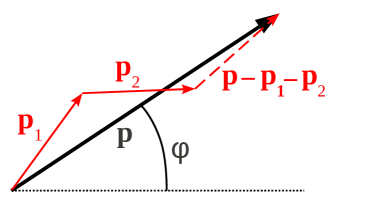
Figure 7: The initial electron momentum ${\rm\bf p}$ (thick solid arrow) with its polar angle $\varphi$ with respect to the $KM$ direction (thin dotted line), and the final momenta of the two electrons ${\rm\bf p}_{1},{\rm\bf p}_{2}$ (thin solid arrows) and of the hole ${\rm\bf p}-{\rm\bf p}_{1}-{\rm\bf p}_{2}$ (thin dashed arrow).

Let $x_{1}p,x_{2}p$ be the projections of ${\rm\bf p}_{1},{\rm\bf p}_{2}$ on ${\rm\bf p}$, and $y_{1}p,y_{2}p$ the projections on the orthogonal direction. The main contribution to the integral in Eq. (16) comes from the region $x_{1},x_{2}>0$, $x_{1}+x_{2}<1$ and $|y_{1}|,|y_{2}|\ll{1}$. Then, we can approximate $|{\rm\bf p}-{\rm\bf p}_{1,2}|\approx{p}(1-x_{1,2})$ in the Coulomb matrix elements, as they are nonsingular in the collinear limit $y_{1,2}\to{0}$. In the energy $\delta$-function, $y_{1,2}$ are kept to the second order:

$$\begin{split}&\epsilon^{e}_{{\rm\bf p}_{1,2}}\approx{v}p\left(x_{1,2}+\frac{y_{1,2}^{2}}{2x_{1,2}}\right),\\ &\epsilon^{h}_{{\rm\bf p}-{\rm\bf p}_{1}-{\rm\bf p}_{2}}\approx{v}p\left[1-x_{1}-x_{2}+\frac{(y_{1}+y_{2})^{2}}{2(1-x_{1}-x_{2})}\right],\end{split}$$

which gives

$$\begin{split}&\mathop{\mathrm{Im}}\nolimits\Sigma_{\rm\bf p}(\epsilon)\approx-\left(\frac{e^{2}}{v}\right)^{2}\frac{vp}{4\pi}{}\times{}\\ &\;\;{}\times{}\int\limits_{0}^{1}dx_{1}\int\limits_{0}^{1-x_{1}}dx_{2}\left[\frac{N}{(1-x_{1})^{2}}-\frac{1}{(1-x_{1})(1-x_{2})}\right]{}\times{}\\ &\;\;{}\times{}\int\limits_{-\infty}^{\infty}{d}y_{1}\,dy_{2}\,\delta\!\left(\frac{\epsilon-vp}{vp}-\frac{y_{1}^{2}}{2x_{1}}-\frac{y_{2}^{2}}{2x_{2}}-\frac{(y_{1}+y_{2})^{2}/2}{1-x_{1}-x_{2}}\right).\end{split}$$

The $y$-integration is performed using the general relation

$$\begin{split}&\int\limits_{-\infty}^{\infty}\delta\!\left(s-\sum_{i,j=1}^{2n}A_{ij}y_{i}y_{j}\right)\prod_{k=1}^{2n}dy_{k}=\\ &=\frac{1}{\sqrt{\det{A}}}\int\limits_{-\infty}^{\infty}\delta\!\left(s-\sum_{i=1}^{2n}\tilde{y}_{i}^{2}\right)\prod_{k=1}^{2n}d\tilde{y}_{k}=\\ &=\frac{\pi^{n}s^{n-1}\,\theta(s)}{\sqrt{\det{A}}\,(n-1)!},\end{split}$$ (17)

valid for any positive-definite $2n\times{2n}$ matrix $A$. The remaining $x$-integration,

$$\begin{split}&\mathop{\mathrm{Im}}\nolimits\Sigma_{\rm\bf p}(\epsilon)\approx-\left(\frac{e^{2}}{v}\right)^{2}\frac{vp}{2}\,\theta(\epsilon-vp)\int\limits_{0}^{1}dx_{1}\int\limits_{0}^{1-x_{1}}dx_{2}{}\times{}\\ &\times\sqrt{x_{1}x_{2}(1-x_{1}-x_{2})}\left[\frac{N}{(1-x_{1})^{2}}-\frac{1}{(1-x_{1})(1-x_{2})}\right],\end{split}$$ (18)

straightforwardly gives Eqs. (6a), (6b).

Eq. (LABEL:detAintegral=) also determines the suppression by energy-momentum conservation of higher-order contributions to $\mathop{\mathrm{Im}}\nolimits\Sigma_{\rm\bf p}(\epsilon\to{vp})$ corresponding to emission of $n$ electron-hole pairs. Indeed, this is precisely the kind of integral one obtains for the perpendicular components of the $2n$ momenta in the collinear limit, with $s\propto(\epsilon-vp)$.

A.3 Second-order self-energy beyond the Dirac approximation

Neglecting the trigonal warping correction to the single-particle eigenstates, one can again use Eq. (16) with the quasiparticle dispersions from Eq. (4) to calculate the self-energy. Using the same notation as in Appendix A.2, we expand the quasiparticle dispersions to the second order in $y_{1},y_{2}$. Consider, for example, $\epsilon^{e}_{{\rm\bf p}_{1}}$:

$$\begin{split}\epsilon^{e}_{{\rm\bf p}_{1}}={}&{}vpx_{1}-(\zeta_{0}+\zeta_{3}\cos{3}\varphi)p^{2}x_{1}^{2}+3\zeta_{3}p^{2}x_{1}y_{1}\sin{3}\varphi{}+{}\\ &{}+{}\left(\frac{vp}{2x_{1}}-\zeta_{0}p^{2}+\frac{7}{2}\,\zeta_{3}p^{2}\cos{3}\varphi\right)y_{1}^{2}.\end{split}$$ (19)

The expression for $\epsilon^{h}_{{\rm\bf p}-{\rm\bf p}_{1}-{\rm\bf p}_{2}}$ has a similar structure. The terms linear in $y_{1},y_{2}$ can be removed by a shift of $y_{1},y_{2}$. Neglecting the terms $\sim(\zeta_{3}p^{2})^{2}/(vp)$ as well as corrections to the determinant in Eq. (LABEL:detAintegral=), we obtain the same Eq. (LABEL:ImS2x=), but with a modified integration domain: in addition to the conditions $x_{1},x_{2}>0$, $x_{1}+x_{2}<1$, there is another condition

$$\epsilon-vp-\zeta_{\varphi}{p}^{2}+2\zeta_{\varphi}{p}^{2}(1-x_{1})(1-x_{2})>0,$$ (20)

where $\zeta_{\varphi}=-\zeta_{0}-\zeta_{3}\cos{3}\varphi$. Even though we could not evaluate the corresponding integral analytically, some general properties of it can be established. First, for sufficiently large negative $\epsilon-vp<-|\zeta_{\varphi}|p^{2}$ the integration domain is empty, so $\mathop{\mathrm{Im}}\nolimits\Sigma_{\rm\bf p}(\epsilon)=0$. Second, for sufficiently large positive $\epsilon-vp>|\zeta_{\varphi}|p^{2}$, the condition (20) becomes redundant, the integration domain coincides with that in Eq. (LABEL:ImS2x=), so $\mathop{\mathrm{Im}}\nolimits\Sigma_{\rm\bf p}(\epsilon)=\gamma_{\rm\bf p}$. Finally, the condition (20) becomes its opposite upon simultaneous change of sign of $\epsilon-vp$ and $\zeta_{\varphi}$. Thus, if one defines a function $\mathcal{F}_{N}(z)$ as

$$\mathcal{F}_{N}(z)=\left[\int\mathcal{I}_{N}(x_{1},x_{2})\,dx_{1}\,dx_{2}\right]^{-1}\times$$

$$\quad{}\times{}\int\theta(z-1+2(1-x_{1})(1-x_{2}))\,\mathcal{I}_{N}(x_{1},x_{2})\,dx_{1}\,dx_{2},$$

(21a)

$$\mathcal{I}_{N}(x_{1},x_{2})\equiv\theta(x_{1})\,\theta(x_{2})\,\theta(1-x_{1}-x_{2})\,\times$$

$$\qquad{}\times{}\sqrt{x_{1}x_{2}(1-x_{1}-x_{2})}{}\times{}$$

$$\qquad{}\times{}\left[\frac{N}{(1-x_{1})^{2}}-\frac{1}{(1-x_{1})(1-x_{2})}\right],$$ (21b)

then $\mathop{\mathrm{Im}}\nolimits\Sigma_{\rm\bf p}(\epsilon)$ is given by Eq. (8).

A.4 Polarization operator in the Dirac approximation

The exact expression for the polarization operator in the Dirac approximation is known since long agoGonzalez1994 :

$$\Pi_{\rm\bf q}(\omega)=-\frac{Nq^{2}/16}{\sqrt{v^{2}q^{2}-\omega^{2}}}.$$ (22)

Still, here we give its simple derivation near the singularity at $\omega\to{vq}$, which will be generalized beyond the Dirac approximation in Sec. A.5. In the collinear approximation the angular factors can be neglected, so the polarization operator is given by

$$\Pi_{\rm\bf q}(\omega)\approx\int\frac{d^{2}{\rm\bf p}}{(2\pi)^{2}}\,\frac{N}{\omega-\epsilon^{e}_{\rm\bf p}-\epsilon^{h}_{{\rm\bf q}-{\rm\bf p}}}.$$ (23)

Let us denote by $xq$ the projection of ${\rm\bf p}$ on ${\rm\bf q}$. and by $yq$ on the orthogonal direction. Then,

$$\begin{split}&\Pi_{\rm\bf q}(\omega)\approx-\frac{Nq}{4\pi^{2}v}\int\limits_{-\infty}^{\infty}{d}x\,dy\times\\ &\qquad{}\times\left(|x|+|1-x|+\frac{y^{2}}{2|x|}+\frac{y^{2}}{2|1-x|}-\frac{\omega}{vq}\right)^{-1}=\\ &=-\frac{Nq}{4\pi{v}}\int\limits_{-\infty}^{\infty}\frac{\sqrt{2|x(1-x)|}\,dx}{\sqrt{(|x|+|1-x|)[|x|+|1-x|-\omega/(vq)]}}=\\ &=-\frac{Nq^{2}}{2\pi\sqrt{2vq(vq-\omega)}}\int\limits_{0}^{1}\sqrt{x(1-x)}\,dx{}-{}\\ &\qquad{}-{}\frac{Nq}{2\pi{v}}\int\limits_{1/2}^{\infty}\frac{\sqrt{u^{2}-1/4}\,du}{\sqrt{u[2u-\omega/(vq)]}}.\end{split}$$

The second term is nonsingular at $\omega\to{v}q$, so it can be ignored (the divergence of the integral is spurious, being a consequence of the collinear approximation). The first one gives $-(Nq^{2}/16)/\sqrt{2vq(vq-\omega)}$, which is precisely Eq. (22) at $\omega\to{vq}$.

A.5 Polarization operator beyond the Dirac approximation

As in Sec. A.4, let us start from Eq. (23) and denote by $xq$ the projection of ${\rm\bf p}$ on ${\rm\bf q}$, and by $yq$ on the orthogonal direction. As in Sec. A.3, let us expand the energies to the second order in $y$, see Eq. (19). In the interval $0<x<1$, which determines the main singularity, we have

$$\epsilon^{e}_{\rm\bf p}+\epsilon^{h}_{{\rm\bf q}-{\rm\bf p}}\approx vq+\zeta_{\varphi}{q}^{2}(2x-1)+\frac{vq}{2}\left(\frac{1}{x}+\frac{1}{1-x}\right)(y-y_{0})^{2},$$

where $y_{0}$ is an $x$-dependent shift. The integration over $y$ is straightforward, the subsequent integral over $x$ reduces to elliptic integrals, to give Eqs. (9a), (9b).

Let us mention some properties of the function $\mathcal{P}(z)$, defined in Eq. (9b). Many of them can be deduced directly from the integral representation,

$$\mathcal{P}(z)=\frac{2}{\pi}\int\limits_{-1}^{1}\sqrt{\frac{1-u^{2}}{u-z}}\,du.$$ (24)

For $z<-1$, $\mathcal{P}(z)$ is purely real, at $z>-1$ it acquires a positive imaginary part whose sign is fixed by the requirement of the analyticity in the upper half-plane of the complex variable $z$, and $\mathcal{P}(z)$ is purely imaginary at $z>1$. The real and imaginary parts are related by $\mathop{\mathrm{Re}}\nolimits\mathcal{F}(-z)=\mathop{\mathrm{Im}}\nolimits\mathcal{F}(z)$. At $z\to-\infty$, $\mathcal{P}(z)\to{1}/\sqrt{-z}$. At $z\to\pm{1}$, $\mathcal{P}(z)$ has a weak singularity:

$$\mathcal{P}(z)\approx\frac{8\sqrt{2}}{3\pi}+\frac{\sqrt{2}\,(z+1)}{\pi}\left[\ln\frac{A}{|z+1|}+i\pi\,\theta(z+1)\right],$$ (25)

with $A\sim{1}$. Finally, there are two integral relations, valid at $y>1$:

$$\int\limits_{-1}^{y}\frac{dz}{\sqrt{y-z}}\,\mathop{\mathrm{Im}}\nolimits\mathcal{P}(z)=\pi,$$ (26a)

$$\int\limits_{-1}^{y}\frac{dz}{\sqrt{y-z}}\,\frac{\mathop{\mathrm{Im}}\nolimits\mathcal{P}(z)}{|\mathcal{P}(z)|^{2}}=\frac{\pi{y}}{2}.$$ (26b)

The first relation can be proven by using Eq. (24) and interchanging the order of integration, while the second relation has been verified numerically.

A.6 RPA self-energy in the Dirac approximation

Upon integration over the internal frequency variable of the RPA diagrams, the self-energy becomes

$$\mathop{\mathrm{Im}}\nolimits\Sigma_{\rm\bf p}(\epsilon)\approx\int\frac{d^{2}{\rm\bf q}}{(2\pi)^{2}}\,V_{\rm\bf q}^{2}\mathop{\mathrm{Im}}\nolimits\frac{\Pi_{\rm\bf q}(\epsilon-\epsilon^{e}_{{\rm\bf p}-{\rm\bf q}})}{1-V_{\rm\bf q}\Pi_{\rm\bf q}(\epsilon-\epsilon^{e}_{{\rm\bf p}-{\rm\bf q}})}.$$ (27)

The imaginary part of the dressed polarization operator is given by

$$\mathop{\mathrm{Im}}\nolimits\frac{\Pi_{\rm\bf q}(\omega)}{1-V_{\rm\bf q}\Pi_{\rm\bf q}(\omega)}=-\frac{Nq^{2}}{16}\,\frac{\sqrt{\omega^{2}-v^{2}q^{2}}}{\omega^{2}-\tilde{v}^{2}q^{2}}\,\theta(\omega-vq),$$

(28a)

$$\frac{\tilde{v}^{2}}{v^{2}}=1-\left(\frac{\pi}{8}\,\frac{Ne^{2}}{v}\right)^{2}.$$ (28b)

Note that $\tilde{v}^{2}$ can become negative, which does not represent any problem; the main effect of $\tilde{v}^{2}$ is to make the denominator nonzero at $\omega\to{v}q$. Because of this, in the resulting expression for the self-energy,

$$\begin{split}\mathop{\mathrm{Im}}\nolimits\Sigma_{\rm\bf p}(\epsilon)\approx{}&{}-\frac{Ne^{4}}{16}\int{d}^{2}{\rm\bf q}\,\theta(\epsilon-v|{\rm\bf p}-{\rm\bf q}|-vq)\times{}\\ {}&{}\times\frac{\sqrt{(\epsilon-v|{\rm\bf p}-{\rm\bf q}|)^{2}-v^{2}q^{2}}}{(\epsilon-v|{\rm\bf p}-{\rm\bf q}|)^{2}-\tilde{v}^{2}q^{2}},\end{split}$$ (29)

one can simply set $\epsilon=vp$ in the denominator and replace the latter by $(v^{2}-\tilde{v}^{2})q^{2}$ provided that $|\epsilon-vp|\ll(Ne^{2}/v)^{2}vq$. This condition will provide a lower cutoff for the integration over $q$.

In the numerator, we approximate

$$(\epsilon-v|{\rm\bf p}-{\rm\bf q}|)^{2}-v^{2}q^{2}\approx 2vq_{\|}(\epsilon-vp)-\frac{p(vq_{\perp})^{2}}{p-q_{\|}},$$

where $q_{\|},q_{\perp}$ are the components of ${\rm\bf q}$ along ${\rm\bf p}$ and perpendicular to ${\rm\bf p}$, respectively, and $|q_{\perp}|\ll{q}_{\|}$. Then after the straightforward integration over $q_{\perp}$, we obtain

$$\begin{split}\mathop{\mathrm{Im}}\nolimits\Sigma_{\rm\bf p}(\epsilon)={}&{}\frac{4(\epsilon-vp)}{\pi{N}}\int\limits_{0}^{p}\frac{dq_{\|}}{q_{\|}}\,\sqrt{\frac{p-q_{\|}}{p}}\approx\\ \approx{}&{}\frac{4(\epsilon-vp)}{\pi{N}}\,\ln\frac{p}{q_{min}},\end{split}$$ (30)

where the logarithmic divergence is cut off at

$$vq_{min}=\max\left\{\epsilon-vp,\frac{\epsilon-vp}{(Ne^{2}/v)^{2}}\right\},$$

as discussed above. Thus, we arrive at Eq. (7).

A.7 RPA self-energy beyond the Dirac approximation

Let us again start from the general Eq. (27). Beyond the Dirac approximation, we use Eq. (9a) and obtain

$$\mathop{\mathrm{Im}}\nolimits\frac{V_{\rm\bf q}^{2}\Pi_{\rm\bf q}(\epsilon-\epsilon^{e}_{{\rm\bf p}-{\rm\bf q}})}{1-V_{\rm\bf q}\Pi_{\rm\bf q}(\epsilon-\epsilon^{e}_{{\rm\bf p}-{\rm\bf q}})}\approx\frac{2\pi{e}^{2}}{q_{\|}}\,\frac{\sqrt{\mathcal{A}}\mathop{\mathrm{Im}}\nolimits\mathcal{P}(z)}{|1+\sqrt{\mathcal{A}}\,\mathcal{P}(z)|^{2}},$$ (31a)

where we denoted

$$\mathcal{A}=\left(\frac{\pi{N}e^{2}}{8v}\right)^{2}\frac{vq_{\|}}{2|\zeta_{\varphi}|q_{\|}^{2}},$$ (31b)

$$z=\frac{1}{|\zeta_{\varphi}|q_{\|}^{2}}\left[\epsilon-vp-\frac{vpq_{\perp}^{2}}{2q_{\|}(p-q_{\|})}-\zeta_{\varphi}(p-q_{\|})^{2}\right].$$

In the relevant region of energies, namely, where Eq. (7) is valid in the Dirac approximation, we have $\mathcal{A}\gg{1}$ and $z\ll\mathcal{A}$. Due to the latter condition and to the fact that $\mathop{\mathrm{Im}}\nolimits\mathcal{P}(z)\sim{1}/\sqrt{z}$ at $z\to\infty$, one can neglect the unity in the denominator of Eq. (31a), which then becomes

$$\mathop{\mathrm{Im}}\nolimits\frac{V_{\rm\bf q}^{2}\Pi_{\rm\bf q}(\epsilon-\epsilon^{e}_{{\rm\bf p}-{\rm\bf q}})}{1-V_{\rm\bf q}\Pi_{\rm\bf q}(\epsilon-\epsilon^{e}_{{\rm\bf p}-{\rm\bf q}})}\approx\frac{16}{N}\sqrt{\frac{2|\zeta_{\varphi}|v}{q_{\|}}}\,\frac{\mathop{\mathrm{Im}}\nolimits\mathcal{P}(z)}{|\mathcal{P}(z)|^{2}}.$$ (32)

Let us pass from the integration over $q_{\perp}$ to the one over $z$, which gives

$$\mathop{\mathrm{Im}}\nolimits\Sigma_{\rm\bf p}(\epsilon)=\frac{8|\zeta_{\varphi}|p^{2}}{\pi^{2}N}\int\limits_{0}^{1}x\sqrt{1-x}\,dx\times$$

$$\qquad{}\times\int\limits_{-1}^{z_{max}}\frac{\theta(z_{max}+1)\,dz}{\sqrt{z_{max}-z}}\,\frac{\mathop{\mathrm{Im}}\nolimits\mathcal{P}(z)}{|\mathcal{P}(z)|^{2}},$$ (33a)

$$z_{max}(x)=\frac{\epsilon-vp-\zeta_{\varphi}p^{2}(1-x)^{2}}{|\zeta_{\varphi}|p^{2}x^{2}}.$$ (33b)

The $z$-integration is performed using Eq. (26b). On the mass shell, $\epsilon=vp+\zeta_{\varphi}{p}^{2}$, the $x$-integral in Eq. (33) converges on the lower limit, and one arrives at Eq. (10).

References

• (1) F. Rana, Phys. Rev. B, 76 155431 (2007).
• (2) P. A. George et al., Nano Lett. 8, 4248 (2008).
• (3) J. W. Dawlaty et al., Appl. Phys. Lett. 92, 042116 (2008).
• (4) D. Sun et al., Phys. Rev. Lett. 101, 157402 (2008).
• (5) Q. Bao et al., Adv. Funct. Mater. 19, 3077 (2009).
• (6) S. Kumar et al., Appl. Phys. Lett. 95, 191911 (2009).
• (7) R. W. Newson, J. Dean, B. Schmidt, and H. M. van Driel, Opt. Express 17, 2326 (2009).
• (8) P. Plochocka et al., Phys. Rev. B 80, 245415 (2009).
• (9) C. H. Lui, K. F. Mak, J. Shan, and T. F. Heinz, Phys. Rev. Lett. 105, 127404 (2010).
• (10) T. Winzer, A. Knorr, and E. Malić, Nano Lett. 10, 4839 (2010).
• (11) P. J. Hale et al., Phys. Rev. B 83, 121404(R) (2011).
• (12) S. Winnerl et al., Phys. Rev. Lett. 107, 237401 (2011).
• (13) M. Breusing et al., Phys. Rev. B 83, 153410 (2011)
• (14) R. Kim, V. Perebeinos, and P. Avouris, Phys. Rev. B 84, 075449 (2011).
• (15) J. H. Strait et al., Nano Lett. 11, 4902 (2011).
• (16) T. Li et al., Phys. Rev. Lett. 108, 167401 (2012).
• (17) T. Winzer, and E. Malić, Phys. Rev. B, 85 241404 (2012).
• (18) J. C. W. Song, K. J. Tielrooij, F. H. L. Koppens, and L. S. Levitov, Phys. Rev. B 87, 155429 (2013).
• (19) D. Brida et al., arXiv:1209.5729.
• (20) K. J. Tielrooij et al., Nature Phys. 9, 248 (2013).
• (21) T. Winzer and E. Malic, J. Phys.: Condens. Matter 25 054201 (2013).
• (22) S. Winnerl et al., J. Phys.: Condens. Matter 25, 054202 (2013).
• (23) B. Y. Sun and M. W. Wu, arXiv:1302.3677.
• (24) E. M. Lifshitz and L. P. Pitaevskii, Statistical Physics Part 2 (Butterworth-Heinemann, Oxford, 1980).
• (25) J. González, F. Guinea, and M. A. H. Vozmediano, Phys. Rev. Lett. 77, 3589 (1996).
• (26) L. Fritz, J. Schmalian, M. Müller, and S. Sachdev, Phys. Rev. B 78, 085416 (2008).
• (27) M. S. Foster and I. L. Aleiner, Phys. Rev. B 79, 085415 (2009).
• (28) D. M. Basko, S. Piscanec, and A. C. Ferrari, Phys. Rev. B 80, 165413 (2009).
• (29) L. E. Golub, S. A. Tarasenko, M. V. Entin, and L. I. Magarill, Phys. Rev. B 84, 195408 (2011).
• (30) U. Fano, Phys. Rev. 124, 1866 (1961); Nuovo Cimento 12, 156 (1935).
• (31) A. Grüneis et al., Phys. Rev. B 78, 205425 (2008).
• (32) D. V. Khveshchenko, Phys. Rev. B 74, 161402(R) (2006).
• (33) S. Das Sarma, E. H. Hwang, and W.-K. Tse, Phys. Rev. B 75, 121406(R) (2007)
• (34) T. Stauber, Phys. Rev. B 82, 201404 (2010).
• (35) G. Gómez-Santos and T. Stauber, Phys. Rev. Lett. 106, 045504 (2011).
• (36) In fact, the ultraviolet divergence in $\mathop{\mathrm{Re}}\nolimits\Sigma_{\rm\bf p}(\epsilon)$ persists to energies of the order of the bandwidth $W$. However, the two contributions to the resulting logarithmic factor, $\ln[W/(\epsilon-vp)]=\ln(W/\xi_{\mathrm{max}})+\ln[\xi_{\mathrm{max}}/(\epsilon-vp)]$ play quite different roles. The first one, $\ln(W/\xi_{\mathrm{max}})$, contributes to the well-known Coulomb renormalization of velocity [see Ref. Gonzalez1994, as well as A. A. Abrikosov and S. D. Beneslavskii, Sov. Phys. JETP 32, 699 (1971); J. González, F. Guinea, and M. A. H. Vozmediano, Phys. Rev. B 59, R2474 (1999); D. C. Elias et al., Nature Phys. 7, 701 (2011)], whose result is that $v$ becomes a slow function of energy. For consistency, the self-energy should also be evaluated on Green’s functions dressed with such logarithmic corrections. The resulting convexity of the spectrum prohibits the quasiparticle decay and suppresses of $\mathop{\mathrm{Im}}\nolimits\Sigma_{\rm\bf p}(\epsilon)$ on the mass shell. Here we are interested in the case when the energy scale of $\epsilon-vp$ on which $\mathop{\mathrm{Im}}\nolimits\Sigma_{\rm\bf p}(\epsilon)$ is suppressed, is smaller than $\gamma_{\rm\bf p}$. Then the main effect of the renormalization, relevant for the present work, is that the Coulomb coupling constant $e^{2}/v$ appearing in all expressions, should be understood as the renormalized value. After that one can focus on the $\ln[\xi_{\mathrm{max}}/(\epsilon-vp)]$ term in $\mathop{\mathrm{Re}}\nolimits\Sigma_{\rm\bf p}(\epsilon)$. Equivalently, one can run the renormalization group on the bare Hamiltonian (2) with the bandwidth $W$ to obtain the renormalized Hamiltonian of the same form, but with the bandwidth $\xi_{\mathrm{max}}$, which then provides the cutoff of the logarithm in $\mathop{\mathrm{Re}}\nolimits\Sigma_{\rm\bf p}(\epsilon)$.
• (37) S. Gangadharaiah, A. M. Farid, and E. G. Mishchenko, Phys. Rev. Lett. 100, 166802 (2008).
• (38) I. Sodemann and M. M. Fogler, Phys. Rev. B 86, 115408 (2012).
• (39) D. M. Basko, Phys. Rev. B 76, 081405(R) (2007); ibid. 78, 125418 (2008).
• (40) P. Venezuela, M. Lazzeri, and F. Mauri, Phys Rev. B 84, 035433 (2011).
• (41) M. Huang, H. Yan, T. F. Heinz, and J. Hone, Nano Lett. 10, 4074 (2010).
• (42) D.Yoon, Y.-W. Son, and H. Cheong, Phys. Rev. Lett. 106, 155502 (2011).
• (43) R. Narula, N. Bonini, N. Marzari, and S. Reich, Phys Rev. B 85, 115451 (2012)
• (44) J. González, F. Guinea, and M. A. H. Vozmediano, Mod. Phys. Lett. B 7, 1593 (1994); Nucl. Phys. B 424, 595 (1994); J. Low Temp. Phys. 99, 287 (1995).