Asymptotic behavior of the Whittle estimator for the increments of a Rosenblatt process

Abstract

The purpose of this paper is to estimate the self-similarity index of the Rosenblatt process by using the Whittle estimator. Via chaos expansion into multiple stochastic integrals, we establish a non-central limit theorem satisfied by this estimator. We illustrate our results by numerical simulations.

2000 AMS Classification Numbers: Primary: 60G18; Secondary 60F05, 60H05, 62F12.

Key words: Whittle estimator; Rosenblatt process; long-memory process; non-central limit theorem; Malliavin calculus.

1 Introduction

The Rosenblatt process appears as limit of normalized sums of long-range dependent series (see [8], [25]). In the last years, this stochastic processes has been the object of several research papers (see [22], [27], [28], [29] among others). Its analysis is motivated by the fact that the Rosenblatt process is self-similar with stationary increments and moreover its exhibits long-range dependence (or long-memory). In this sense, it shares many properties with the more known fractional Brownian motion (fBm in the sequel) except the fact that the Rosenblatt process is not a Gaussian process. Recall that the fBm is the only Gaussian self-similar process with stationary increments.

The practical aspects of Rosenblatt process are striking: it provides a new class of processes from which to model long memory, self-similarity, and Hölder-regularity, allowing significant deviation from fBm and other Gaussian processes. The need of non-Gaussian self-similar processes in practice (for example in hydrology) is mentioned in the paper [26] based on the study of stochastic modeling for river-flow time series in [15].

The Hurst parameter $H$ characterizes all the important properties of a Rosenblatt process, as seen above. Therefore, estimating $H$ properly is an important problem in the analysis of this process. The Hurst parameter estimation from a $N$-length path of a fBm or more generally of self-similar or long-range dependent processes, has a long history. Several statistics have been introduced and studied to this end, such as parametric estimators (maximum likelihood estimator) as well as semi-parametric estimators (spectral, variogram or wavelets based estimators). Informations on these various approaches can be found in the books of Beran [4] or Doukhan et al. [10]. But in the particular case of the fBm, the main results concerning this estimation were certainly obtained by [11] and [7]. Indeed the optimal method for estimating $H$ is obtained from the maximization of the Whittle approximation of the log-likelihood introduced by Whittle in [30] (in the sequel, the Whittle estimator). This estimator shares the same asymptotic behavior than the maximum likelihood estimator (MLE), notably it is asymptotically efficient, but numerically the Whittle estimator is clearly many more interesting than the MLE (no need to inverse the covariance matrix). These properties also hold for long memory stationary Gaussian processes as it was established in [11] and [7] under almost general conditions: the Whittle estimator is asymptotically normal with a $\sqrt{N}$ convergence rate.

In the case of long memory non-Gaussian time series, there exist very few results concerning the limit behavior of the Whittle estimator. In [13], the case of fourth order moment linear processes have been considered and it was proved that the Whittle estimator is still asymptotically normal with a $\sqrt{N}$ convergence rate. But in [14], the cases of functionals of long memory Gaussian processes have been studied and the conclusion is different: in general, the Whittle estimator satisfies a non-central limit theorem with a non Gaussian limit distribution and a convergence rate smaller than $\sqrt{N}$. This is notably the case when the functional is the Hermite polynomial $H_{2}(x)=x^{2}-1$.

Estimating the memory parameter of the Rosenblatt process appears to be a challenging problem. This is due to the fact that this process is not a Gaussian process, the explicit expression of its probability density is not know and standard techniques cannot be applied in this case. The development of new criteria, based on the Malliavin calculus and chaos expansion into multiple Wiener-Itô integrals (see the monograph [17]), for the convergence of sequences of random variables recently led to new results. In [28] and [6] the authors studied the asymptotic behavior of the quadratic variations of the Rosenblatt process in order to obtain the asymptotic properties of an estimator for the self-similarity index. An approach based on wavelets has been also proposed in [3]. A common denominator of all these works is that the estimators constructed are consistent but in general their limit behavior is not Gaussian. This not very convenient for practical aspects.

We want to put a new brick to the theory of the long-memory parameter estimation for non-Gaussian stochastic processes. We analyze the limit behavior of the Whittle estimator for the self-similarity index $H$ of the increments of a Rosenblatt process (where $0.5<H<1$). We will see that, as in the case of the estimators based on the quadratic variations (see [28]), the Whittle estimator has a non-Gaussian limit behavior and the convergence rate is $N^{1-H}$. This is due to the fact that, if one compares with the fBm case, the chaos expansion of the estimator involves a new term with a strong dependence structure that cannot be compensated by the smoothness of the estimator. This result is not totally surprising. Indeed, from [25], the Rosenblatt can be obtained as the limit of $\frac{1}{n}\sum_{k=1}^{[nt]}H_{2}(X_{k})$ when $n\to\infty$, where $(X_{k})$ is a long memory Gaussian process and we know from [14] that the Whittle estimator of $(H_{2}(X_{k}))_{k}$ also satisfies the same kind of non- central limit theorem.

Unfortunately, our new result concerning the Whittle estimator keeps open the following question: is it possible to propose an asymptotically Gaussian estimator of the self-similarity parameter of a Rosenblatt process? However, Monte-Carlo experiments attests that the Whittle estimator numerically provides accurate estimations, clearly better than with other well known estimators and with almost the same quality than the one obtained for the fBm when $H$ is close to $0.5$. Hence, even if it asymptotically satisfies a non-central limit theorem, the Whittle estimator is really interesting for estimating the $H$ parameter of a Rosenblatt process.

We organized our paper as follows. Section 2 contains some preliminaries on multiple stochastic integrals, the Rosenblatt process and the Whittle estimator. In Section 3 we analyze the asymptotic behavior of the Whittle estimator for the self-similarity index. Finally, Section 4 contains a numerical study of the estimator and main proofs of this paper are established in Section 5.

2 Preliminaries

In this section we introduce the basic concepts used throughout the paper. We will present the the multiple stochastic integrals, the definition and the immediate properties of the Rosenblatt process and the basic facts concerning the Whittle estimator.

To begin with we call back some elements about multiple stochastic integrals.

2.1 Multiple stochastic integrals

Let $W=(W_{t})_{t\in\mathbb{R}}$ be a classical Wiener process on a standard probability space $\left(\Omega,{\mathcal{F}},\mathbf{P}\right)$. If $f\in L^{2}(\mathbb{R}^{n})$ with $n\geq 1$ integer, we introduce the multiple Wiener-Itô integral of $f$ with respect to $W$. The basic reference is the monograph [18]. Let $f\in{\mathcal{S}_{n}}$ be an elementary function with $n$ variables that can be written as $f=\sum_{i_{1},\ldots,i_{n}}c_{i_{1},\ldots,i_{n}}1_{A_{i_{1}}\times\ldots\times A_{i_{n}}}$, where the coefficients satisfy $c_{i_{1},\ldots,i_{n}}=0$ if two indexes $i_{k}$ and $i_{l}$ are equal and the sets $A_{i}\in{\mathcal{B}}(\mathbb{R})$ are pairwise disjoint. For such a step function $f$ we define

$$I_{n}(f)=\sum_{i_{1},\ldots,i_{n}}c_{i_{1},\ldots,i_{n}}W(A_{i_{1}})\ldots W(A_{i_{n}})$$

where we put $W(A)=\int_{\mathbb{R}}1_{A}(s)dW_{s}$. It can be seen that the application $I_{n}$ constructed above from ${\mathcal{S}}_{n}$ to $L^{2}(\Omega)$ is an isometry on ${\mathcal{S}}_{n}$ in the sense

$$I\!\!E\,\left[I_{n}(f)I_{m}(g)\right]=n!\langle f,g\rangle_{L^{2}(T^{n})}\quad\mbox{ if }m=n$$ (1)

and

$$I\!\!E\,\left[I_{n}(f)I_{m}(g)\right]=0\quad\mbox{ if }m\not=n.$$

Since the set ${\mathcal{S}_{n}}$ is dense in $L^{2}(\mathbb{R}^{n})$ for every $n\geq 1$ the mapping $I_{n}$ can be extended to an isometry from $L^{2}(\mathbb{R}^{n})$ to $L^{2}(\Omega)$ and the above properties hold true for this extension.
It also holds that $I_{n}(f)=I_{n}\big{(}\tilde{f}\big{)}$, where $\tilde{f}$ denotes the symmetrization of $f$ defined by

$$\tilde{f}(x_{1},\ldots,x_{n})=\frac{1}{n!}\sum_{\sigma}f(x_{\sigma(1)},\ldots,x_{\sigma(n)}),$$

$\sigma$ running over all permutations of $\left\{1,...,n\right\}$. We will need the general formula for calculating products of Wiener chaos integrals of any orders $m,n$ for any symmetric integrands $f\in L^{2}(\mathbb{R}^{m})$ and $g\in L^{2}(\mathbb{R}^{n})$, which is

$$I_{m}(f)I_{n}(g)=\sum_{\ell=0}^{m\wedge n}\ell!\binom{m}{\ell}\binom{n}{\ell}I_{m+n-2\ell}(f\otimes_{\ell}g),$$ (2)

where the contraction $f\otimes_{\ell}g$ is defined by

$$(f\otimes_{\ell}g)(s_{1},\ldots,s_{m-\ell},t_{1},\ldots,t_{n-\ell})$$

$$=\int_{T^{m+n-2\ell}}f(s_{1},\ldots,s_{m-\ell},u_{1},\ldots,u_{\ell})g(t_{1},\ldots,t_{n-\ell},u_{1},\ldots,u_{\ell})du_{1}\ldots du_{\ell}$$ (3)

and by extension $f\otimes_{0}g=f\otimes g$. Note that the contraction $(f\otimes_{\ell}g)$ is an element of $L^{2}(\mathbb{R}^{m+n-2\ell})$ but it is not necessarily symmetric. We will denote its symmetrization by $(f\tilde{\otimes}_{\ell}g)$.

2.2 The Rosenblatt process

Recall that a fBm $B=(B_{t})_{t\geq 0}$ with Hurst parameter $H\in(\frac{1}{2},1)$ and parameter $C>0$ is a centered Gaussian process with covariance function

$$\mbox{Cov}\,(B_{t},B_{s})=I\!\!E\,(B_{t}B_{s})=\frac{C^{2}}{2}\big{(}s^{2H}+t^{2H}-|t-s|^{2H}\big{)},\quad s,t\in[0,\infty),$$ (4)

with $C=\mbox{Var}\,(B_{1})$. It is the only normalized Gaussian $H$-self-similar process with stationary increments. The fBm admits the following moving average representation: for every $t\geq 0$ and for every $H>\frac{1}{2}$

$$B_{t}=Cc_{B}(H)\int_{\mathbb{R}}\left(\int_{0}^{t}(u-y)_{+}^{H-\frac{3}{2}}du\right)dW(y).$$ (5)

where $(W(y),y\in\mathbb{R})$ is a standard Brownian motion with time interval $\mathbb{R}$ and $c_{B}(H)$ is a strictly positive constant that ensures that $E(B_{t})^{2}=C^{2}t^{2H}$ for every $t\geq 0$.

The Rosenblatt process is related to the fractional Brownian motion. It shares many properties of the fBm. For instance, it has the same covariance function (4) as the fBm, it is $H$-self-similar and it has stationary increments. It has the same order of the Hölder regularity of its sample paths as the fBm (that is, the Rosenblatt process, as well as the fBm, are Hölder continuous of order $\delta$ with $0<\delta<H$). There are also some differences with respect to the fBm. One of them, is that it is defined only for the self-similarity index $H>\frac{1}{2}$ and another difference, more important, is that it is not Gaussian. It can be expressed as a double multiple integral with respect to the Wiener process and therefore it is an element of the second Wiener chaos. More exactly, a Rosenblatt process $Z=(Z_{t})_{t\geq 0}$ with self-similarity order $H\in(\frac{1}{2},1)$ and parameter $C>0$ is defined by

$$Z_{t}=Cc_{Z}(H)\int_{\mathbb{R}}\int_{\mathbb{R}}\left(\int_{0}^{t}(u-y_{1})_{+}^{\frac{H}{2}-1}(u-y_{2})_{+}^{\frac{H}{2}-1}du\right)dW(y_{1})dW(y_{2})$$ (6)

where $c_{Z}(H)$ is a strictly positive constant such that $E(Z_{1})^{2}=C^{2}$, i.e.

$$c^{2}_{Z}(H)=\frac{2H(2H-1)}{\beta^{2}(1-H,\frac{H}{2})}\qquad\mbox{see e.g. \cite[cite]{[\@@bibref{}{T}{}{}]}}.$$ (7)

We will call a (standard) Rosenblatt random variable every random variable that has the same law as $Z_{1}$ with parameter $C=1$. In the sequel we will use the kernel $L_{H}$ of the Rosenblatt process defined by

$$L^{H}(y_{1},y_{2})=\int_{0}^{t}(u-y_{1})_{+}^{\frac{H}{2}-1}(u-y_{2})_{+}^{\frac{H}{2}-1}du\qquad\mbox{for $(y_{1},y_{2})\in\mathbb{R}^{2}$.}$$ (8)

As the second order properties of a Rosenblatt process are the same than the ones of the corresponding fBm, the process $Y=(Y_{t})_{t\geq 0}$ of the increments of a Rosenblatt process, defined by

$$Y_{t}=Z_{t+1}-Z_{t}\qquad\mbox{for $t\geq 0$}$$

with $Z_{0}=0$ by definition, is a long memory stationary process with covariogram

$$r_{H,C}(t):=\mbox{Cov}\,(Y_{0},\,Y_{t})=\frac{C^{2}}{2}\,\big{(}|t+1|^{2H}+|t-1|^{2H}-2|t|^{2H}\big{)}\quad\mbox{for $t\in\mathbb{R}$},$$ (9)

and a spectral density $f_{H,C}$ defined for $\lambda\in[-\pi,\pi]$ by:

$$f_{H,C}(\lambda):=\frac{1}{2\pi}\,\sum_{k\in\mathbb{Z}}r(k)\,e^{ik\lambda}=\frac{C^{2}\,H\Gamma(2H)\sin(\pi H)}{2\pi}\,(1-\cos\lambda)\sum_{k\in\mathbb{Z}}|\lambda+2k\pi|^{-1-2H},$$ (10)

since $\int_{\mathbb{R}}(1-\cos x)|x|^{-1-2H}dx=2\pi\big{(}H\Gamma(2H)\sin(\pi H)\big{)}^{-1}$ (see Sinai, 1976, or Fox and Taqqu, 1986).

2.3 The Whittle estimator

Our purpose is to study the asymptotic properties of the Whittle estimator of parameters $H$ and $C$ computed from a sample $(Z_{1},\cdots,Z_{N})$ of a Rosenblatt process $Z=(Z_{t})_{t\geq 0}$ . Let us briefly introduce the Whittle estimator. The first step is to define the periodogram of the process $Y$ of the increments of $Z$:

$$\widehat{I}_{N}(\lambda)=\frac{1}{2\pi\,N}\Big{|}\sum_{k=0}^{N-1}Y_{k}\,e^{-ik\lambda}\Big{|}^{2}$$ (11)

Now, let $g:\mathbb{R}\rightarrow\mathbb{R}$ be a $2\pi$-periodic function such that $g\in\mathbb{L}^{2}([-\pi,\pi])$ and define

$$\widehat{J}_{N}(g) = \int_{-\pi}^{\pi}g(\lambda)\widehat{I}_{n}(\lambda)\,d\lambda,~{}~{}~{}\mbox{the integrated periodogram of}~{}Y$$

$$\mbox{and}~{}~{}J(g) = \int_{-\pi}^{\pi}g(\lambda)f_{H,C}(\lambda)\,d\lambda,$$

with $f_{H,C}$ denotes the spectral density of $Y$ defined in (10). From (9) and (11), we also have

$${\widehat{I}_{N}(\lambda)=\frac{1}{2\pi}\sum_{|k|<N}\widehat{r}_{N}(k)e^{-ik\lambda}~{}~{}\mbox{with}~{}~{}\widehat{r}_{N}(k)=\frac{1}{N}\sum_{j=1}^{N-|k|}Y_{j}Y_{j+|k|}},$$ (12)

which is a biased estimate of $r_{H,C}(k)$ (see the next section). Thus, the periodogram $\widehat{I}_{N}(\lambda)$ could be a natural estimator of the spectral density; unfortunately it is not a consistent estimator. However, once integrated with respect to some $\mathbb{L}^{2}$ function, its behavior becomes quite smoother and can allow an estimation of the spectral density. The Whittle’s contrast is a special case of the integrated periodogram $\widehat{J}_{N}(g)$. Indeed, this contrast can be written (see [30])

$$\widehat{U}_{N}(H,C)=\int_{-\pi}^{\pi}\Big{(}\log(f_{H,C}(\lambda))+\widehat{J}_{N}(1/f_{H,C}(\lambda))\Big{)}d\lambda.$$

The Whittle estimator is thus:

$$(\widehat{H}_{N},\widehat{C}_{N}):=\mbox{Argmin}_{(H,C)\in(1/2,1)\times(0,\infty)}\widehat{U}_{N}(H,C).$$

But using a classical renormalization (see Fox and Taqqu, 1986 for instance), the spectral density $f_{H,C}$ of $Y$ can be decomposed as:

$$f_{H,C}(\lambda) = \sigma^{2}\,g_{H}(\lambda)\quad\mbox{with}\left\{\begin{array}[]{lll}\sigma^{2}&=&\displaystyle\frac{1}{2\pi}\,\frac{C^{2}}{a_{H}}H\Gamma(2H)\sin(\pi H)\vspace{0.2cm}\\ g_{H}(\lambda)&=&\displaystyle a_{H}(1-\cos\lambda)\sum_{k\in\mathbb{Z}}|\lambda+2k\pi|^{-1-2H}\\ \end{array}\right.$$ (15)

for all $\lambda\in[-\pi,0)\cup(0,\pi]$ with $\displaystyle a_{H}:=\exp\Big{[}-\int_{-\pi}^{\pi}\log\Big{(}(1-\cos t)\sum_{k\in\mathbb{Z}}\big{|}t+2k\pi\big{|}^{-1-2H}\Big{)}dt\Big{]}$.
Then

$$\int_{-\pi}^{\pi}\log(g_{H}(\lambda))d\lambda=0$$ (16)

for $H\in(1/2,1)$ and the minimization of $\widehat{U}_{N}(H,C)$ can be write again as a minimization in $(H,\sigma^{2})$ and this implies that

$$\widehat{H}_{N} = \mbox{Argmin}_{H\in(1/2,1)}\left\{\widehat{J}_{N}(1/g_{H})\right\}=\mbox{Argmin}_{H\in(1/2,1)}\Big{\{}\int_{-\pi}^{\pi}\frac{\widehat{I}_{N}(\lambda)}{g_{H}(\lambda)}\,d\lambda\Big{\}}$$ (17)

$$~{}~{}\mbox{and}~{}~{}~{}\widehat{C}_{N} = \Big{(}2\pi\,\frac{a_{\widehat{H}_{N}}\,\widehat{\sigma}^{2}_{N}}{{\widehat{H}_{N}}\Gamma(2{\widehat{H}_{N}})\sin(\pi{\widehat{H}_{N}})}\Big{)}^{1/2}\qquad\mbox{with}\qquad\widehat{\sigma}^{2}_{N}:=\frac{1}{2\pi}\widehat{J}_{N}(1/g_{\widehat{H}_{N}}).$$ (18)

Remark 1

However, for practical use, these definitions $\widehat{H}_{N}$ and $\widehat{\sigma}^{2}_{N}$ have to be modified. Indeed, the assumption that the process has zero mean is unrealistic. Moreover, the integrals defining the estimators has to be replaced by their approximations by a Riemann sum. Thus, define:

$$\widetilde{H}_{N}~{} = \mbox{Argmin}_{H\in(1/2,1)}\Big{\{}\frac{2\pi}{N}\,\sum_{k=1}^{N}\frac{\widetilde{I}_{N}(\pi k/N)}{g_{H}(\pi k/N)}\Big{\}}~{}~{}~{}\mbox{and}~{}~{}~{}\widetilde{\sigma}^{2}_{N}=\frac{1}{N}\,\sum_{k=1}^{N}\frac{\tilde{I}_{N}(\pi k/N)}{g_{\widetilde{H}_{N}}(\pi k/N)},$$

$$\mbox{with}~{}~{}\widetilde{I}_{N}(\lambda)=\frac{1}{2\pi\,N}\Big{|}\sum_{k=0}^{N-1}(Y_{k}-\overline{Y}_{N})e^{-ik\lambda}\Big{|}^{2}~{}~{}\mbox{for}~{}\lambda\in[-\pi,\pi]~{}~{}\mbox{and}~{}~{}\overline{Y}_{N}=\frac{1}{N}\,\sum_{k=0}^{N-1}Y_{k}.$$

3 Limit theorems for the Whittle estimator of parameters of a Rosenblatt process

In this section, we prove limit theorems for the integrated periodogram $\widehat{J}_{N}(g)$ for $g\in\mathbb{L}^{2}[-\pi,\pi])$ satisfying certain conditions. Applied to $g=1/g_{H}$, we will prove the almost-sure convergence of $\widehat{H}_{N}$. Applied to $g=\frac{\partial}{\partial H}(1/g_{H})$ and then with a classical Taylor expansion also using the case $g=\frac{\partial^{2}}{\partial^{2}H}(1/g_{H})$ this will provide a non-central limit theorem satisfied by $\widehat{H}_{N}$.
 
Therefore, the main point is to obtain limit theorems for $\widehat{J}_{N}(g)$ . For this, we use a (now) standard approach based on the chaotic decomposition of the random variable $\widehat{J}_{N}$ into a sum of multiple stochastic integrals. Since the Rosenblatt process at fixed time is a multiple integral of order $2$, the product $Y_{j}Y_{j+k}$ is a product of two double multiple integrals which can be expressed as a the sum of a multiple integral of order $4$, a multiple integral of order $2$ and a deterministic function, which is the expectation of $Y_{j}Y_{j+k}$. This decomposition is transferred to the integrated periodogram $\widehat{J}_{N}$, which will be written as sum of two multiple integrals (one of order 2, one of order 4) plus its expectation. What we do next, is to analyze these three terms that compose $\widehat{J}_{N}$. We will see that, as in the case of the variation statistic of the Rosenblatt process (see [28]) or of wavelet statistic (see [3]), the dominant term is the one in the second Wiener chaos, which will give the asymptotic behavior of $\widehat{J}_{N}$. A detailed study of this term shows that it converges to a Rosenblatt random variable.

3.1 Chaos decomposition of the integrated periodogram

The purpose of this part is to provide the asymptotic behavior of a sequence $\widehat{J}_{N}(g)$ using its chaos decomposition. We start first with the analysis of $\widehat{r}_{N}(k)$ with fixed $k\in\mathbb{Z}$. We will study the convergence of $\widehat{r}_{N}(k)$ to the covariance function $r_{H,C}(k)$. We first observe that

$$I\!\!E\,\widehat{r}_{N}(k)=\frac{1}{N}\sum_{j=0}^{N-|k|-1}I\!\!E\,Y_{j}Y_{j+|k|}=\frac{N-|k|}{N}r_{H,C}(k)$$

and this converges to $r_{H,C}(k)$ when $N\to\infty$: $\widehat{r}_{N}(k)$ is an asymptotically unbiased estimator for $r_{H,C}(k)$. On the other hand, for every $j\geq 1$ we can write the increment of the Rosenblatt process as

$$Y_{j}=Z_{j+1}-Z_{j}=I_{2}(\Delta L_{j}^{H})$$

where $L^{H}$ is the kernel of the Rosenblatt process (8) and we denoted by $\Delta L^{H}_{j}$ the two-variables kernel

$$\Delta L^{H}_{j}(y_{1},y_{2}) = C\,c_{Z}(H)\int_{j}^{j+1}(u-y_{1})_{+}^{\frac{H}{2}-1}(u-y_{2})_{+}^{\frac{H}{2}-1}du.$$

In the sequel we will simply denote $L^{H}:=L$. Then, for every $|k|<N$, by the product formula (2)

$$\widehat{r}_{N}(k)-r_{H,C}(k) = \frac{1}{N}\sum_{j=0}^{N-|k|-1}I_{2}(\Delta L_{j})I_{2}(\Delta L_{j+|k|})$$

$$= \frac{1}{N}\sum_{j=0}^{N-|k|-1}\big{(}I_{4}(\Delta L_{j}\otimes\Delta L_{j+|k|})+4\,I_{2}(\Delta L_{j}\otimes_{1}\Delta L_{j+|k|})\big{)}$$

$$+I\!\!E\,\widehat{r}_{N}(k)-r_{H,C}(k).$$

Therefore, for $g\in\mathbb{L}^{2}([-\pi,\pi])$,

$$\widehat{J}_{N}(g)-I\!\!E\,\widehat{J}_{N}(g) = \frac{1}{2\pi\,N}\int_{-\pi}^{\pi}d\lambda g(\lambda)\sum_{|k|<N}\sum_{j=0}^{N-|k|-1}e^{ik\lambda}\ \big{(}I_{4}(\Delta L_{j}\otimes\Delta_{j+|k|}L)+4\,I_{2}(\Delta L_{j}\otimes_{1}\Delta L_{j+|k|})\big{)}~{}~{}~{}$$

$$= \widehat{T}_{2,N}(g)+\widehat{T}_{2,N}(g),$$

$$\mbox{where}\qquad\widehat{T}_{4,N}(g) := \frac{1}{2\pi\,N}\int_{-\pi}^{\pi}d\lambda g(\lambda)\sum_{|k|<N}\sum_{j=0}^{N-|k|-1}e^{ik\lambda}\ I_{4}\Big{(}\Delta L_{j}(y_{1},y_{2})\Delta L_{j+|k|}(y_{1},y_{2})\Big{)}$$ (20)

$$\mbox{and}\qquad\widehat{T}_{2,N}(g) := \frac{2}{\pi\,N}\int_{-\pi}^{\pi}d\lambda g(\lambda)\sum_{|k|<N}\sum_{j=0}^{N-|k|-1}e^{ik\lambda}\ I_{2}\Big{(}\int_{\mathbb{R}}dx\Delta L_{j}(y_{1},x)\Delta L_{j+|k|}(y_{2},x)\Big{)}.$$ (21)

The notation $\widehat{T}_{2,N}(g),~{}\widehat{T}_{4,N}(g)$ suggests that the sequence $\widehat{T}_{4,N}(g)$ belongs to the fourth Wiener chaos while $\widehat{T}_{2,N}(g)$ belongs to the second Wiener chaos.

3.2 Asymptotic behavior of the integrated periodogram

In order to study the asymptotic behavior of $\widehat{J}_{N}(g)$ let us first specify our assumptions on the function $g$. For $H\in(1/2,1)$ and for $g:[-\pi,\pi]\mapsto\mathbb{R}$, we introduce
 
Assumption A$(H)$: $g\in\mathbb{L}^{2}([-\pi,\pi])$ and for any $\delta>0$, there exists $C$ such that

$$|g(\lambda)|\leq C\,|\lambda|^{2H-1-\delta}\qquad\mbox{for all $\lambda\in[-\pi,0)\cup(0,\pi]$.}$$

A very useful point for us is the following (already proved in [12], p. 531):

Lemma 1

Let $H\in(1/2,1)$ and let $g_{H}$ be given by (10). Then, $1/g_{H}$, $\frac{\partial}{\partial H}(1/g_{H})$ and $\frac{\partial^{2}}{\partial H^{2}}(1/g_{H})$ satisfy Assumption A$(H)$.

The limit in distribution of the sequence $\widehat{J}_{N}(g)-I\!\!E\,\widehat{J}_{N}(g)$ as $N\to\infty$ depends on the asymptotic behavior of the two terms $\widehat{T}_{2,N}(g)$ and $\widehat{T}_{4,N}(g)$ above. First, let us analyze the term in the second Wiener chaos, denoted by $\widehat{T}_{2,N}(g)$, of the decomposition $\widehat{J}_{N}(g)$ when the function $g$ satisfies Assumption A$(H)$. Its asymptotic behavior is described by the following result.

Proposition 1

For every $H\in(\frac{1}{2},1)$ and all function $g$ satisfying Assumption A$(H)$,

$$N^{1-H}\,\widehat{T}_{2,N}(g)\begin{array}[t]{c}\stackrel{{\scriptstyle{\cal D}}}{{\longrightarrow}}\\ {\scriptstyle N\rightarrow\infty}\end{array}8\,\sqrt{\frac{2(2H-1)}{H(1-H)^{2}}}\,\Big{(}\int_{-\pi}^{\pi}g(\lambda)f_{(H+1)/2,C}(\lambda)\,d\lambda\Big{)}\,R,$$

with $R$ a standard Rosenblatt random variable $(I\!\!E\,R^{2}=1$).

Under the normalization of $\widehat{T}_{2,N}(g)$ the summand $\widehat{T}_{4,N}(g)$ goes to zero:

Proposition 2

For every $H\in(\frac{1}{2},1)$ and all function $g$ satisfying Assumption A$(H)$,

$$N^{1-H}\,\widehat{T}_{4,N}(g)\begin{array}[t]{c}\stackrel{{\scriptstyle\mathbb{L}^{2}(\Omega)}}{{\longrightarrow}}\\ {\scriptstyle N\rightarrow\infty}\end{array}0.$$

A non-central limit theorem satisfied by $\widehat{J}_{N}(g)$ is thus the consequence of both the previous Propositions 1 and 2:

Proposition 3

For every $H\in(\frac{1}{2},1)$ and all function $g$ satisfying Assumption A$(H)$,

$$N^{1-H}\,\big{(}\widehat{J}_{N}(g)-I\!\!E\,\widehat{J}_{N}(g)\big{)}\begin{array}[t]{c}\stackrel{{\scriptstyle{\cal D}}}{{\longrightarrow}}\\ {\scriptstyle N\rightarrow\infty}\end{array}8\,\sqrt{\frac{2(2H-1)}{H(1-H)^{2}}}\,\Big{(}\int_{-\pi}^{\pi}g(\lambda)f_{(H+1)/2,C}(\lambda)\,d\lambda\Big{)}\,R,$$

with $R$ a standard Rosenblatt random variable $(I\!\!E\,R^{2}=1$).

The above Proposition 3 holds for any function $g$ that satisfies Assumption A(H). The next result shows that, when $g=\frac{1}{\partial H}\left(\frac{1}{g_{H}}\right)$ (with $g_{H}$ defined in (15)) under the normalization of $\widehat{T}_{2,N}(g)$ the deterministic term in the chaos expansion of $\widehat{J}_{N}(g)$ converges to zero.

Proposition 4

With $g_{H}$ given by (10), we have

$$N^{1-H}\,I\!\!E\,\widehat{J}_{N}\Big{(}\frac{\partial}{\partial H}\big{(}\frac{1}{g_{H}}\big{)}\Big{)}\begin{array}[t]{c}\stackrel{{\scriptstyle}}{{\longrightarrow}}\\ {\scriptstyle N\rightarrow\infty}\end{array}0.$$

It is also possible to show the following almost sure limit theorem for the sequence $\widehat{J}_{N}(g)$ when $g$ satisfies Assumption A(H).

Proposition 5

For every $H\in(\frac{1}{2},1)$ and all function $g$ satisfying Assumption A$(H)$, we have

$$\widehat{J}_{N}(g)\begin{array}[t]{c}\stackrel{{\scriptstyle{a.s.}}}{{\longrightarrow}}\\ {\scriptstyle N\rightarrow\infty}\end{array}\sigma^{2}\int_{-\pi}^{\pi}g(\lambda)\,g_{H}(\lambda)\,d\lambda.$$

Now, we can state our main result.

Theorem 1

Let $\widehat{H}_{N}$ be defined by (17). Then

$$\widehat{H}_{N}\begin{array}[t]{c}\stackrel{{\scriptstyle{a.s.}}}{{\longrightarrow}}\\ {\scriptstyle N\rightarrow\infty}\end{array}H\qquad\mbox{and}\qquad N^{1-H}\,\big{(}\widehat{H}_{N}-H\big{)}\begin{array}[t]{c}\stackrel{{\scriptstyle{\cal D}}}{{\longrightarrow}}\\ {\scriptstyle N\rightarrow\infty}\end{array}\gamma(H)\,R$$

where $R$ is a standard Rosenblatt random variable (with $I\!\!E\,R^{2}=1$) and $\gamma(H)$ is defined by:

$$\gamma(H):=16\pi\,\sqrt{\frac{2(2H-1)}{H(1+H)^{2}}}\,\Big{(}\int_{-\pi}^{\pi}\frac{f_{(H+1)/2,1}(\lambda)}{g_{H}(\lambda)}\,d\lambda\Big{)}\,\Big{(}\int_{-\pi}^{\pi}f_{H,1}(\lambda)\frac{\partial^{2}}{\partial H^{2}}\left(\frac{1}{g_{H}(\lambda)}\right)d\lambda\Big{)}^{-1}$$ (22)

It is also possible to provide the strong convergence of $\widehat{C}_{N}$ (defined in 18) to $C$:

Corollary 1

Under the assumptions of Theorem 1,

$$\widehat{C}_{N}\begin{array}[t]{c}\stackrel{{\scriptstyle{a.s.}}}{{\longrightarrow}}\\ {\scriptstyle N\rightarrow\infty}\end{array}C\qquad\mbox{and}\qquad N^{1-H}\,\big{(}\widehat{C}_{N}-C\big{)}\begin{array}[t]{c}\stackrel{{\scriptstyle{\cal D}}}{{\longrightarrow}}\\ {\scriptstyle N\rightarrow\infty}\end{array}C\,\rho(H)\,R,$$

where $R$ is a standard Rosenblatt random variable (with $I\!\!E\,R^{2}=1$) and $\rho(H)$ is defined in (47).

4 Monte-Carlo experiments

We generated $200$ paths of Rosenblatt processes for several values of $H$ ($=0.55$, $0.65,\cdots,0.95$) and $N$ $(=1000,\,5000$ and $20000$). These paths are obtained from the algorithm already used in [3] and deduced from the asymptotic behavior of $n^{-H}\sum_{i=1}^{[nt]}(Y_{i}^{2}-1)$ when $n\to\infty$ where $(Y_{i})$ is a sequence of centered and normalized LRD processes with memory parameter $d=H/2$ (typically FARIMA$(0,H/2,0)$ processes). Note that the generator of Rosenblatt process paths as well as the computations of the estimators used in this section are available on the website http://samm.univ-paris1.fr/-Jean-Marc-Bardet with a free access on (in Matlab language).
We computed the Whittle estimator $\widehat{H}_{N}$ of $H$. An example of the estimation of the probability density function of $\widehat{H}_{N}$ provided by the Silverman’s nonparametric procedure is given in Figure 1. This estimated probability density function appears could first appear as Gaussian density function but it is slightly asymmetric as the Rosenblatt density function should be when $H=0.65$ (see for instance Figure 1 in [29]).

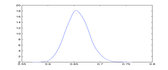
Figure 1: FFT estimation (Silverman’s method) of the density of the limit of $\widehat{H}_{N}$ for $H=0.65$, $N=5000$ from $1000$ independent replications of Rosenblatt process paths.

The Whittle estimator $\widehat{H}_{N}$ of $H$ applied to paths of Rosenblatt processes is also compared to both other estimators:

• The extended local Whittle estimator $\widehat{H}_{ADG}$ defined in [1] from the seminal paper [23]. The trimming parameter is chosen as $m=N^{0.65}$ (this is not an adaptive estimator) following the numerical recommendations of [1].

• The wavelet estimator $\widehat{H}_{Wa}$ as it was already defined in [3].

Note that both these estimators are semi-parametric estimators (while $\widehat{H}_{N}$ is a parametric estimator) and thus can be applied to other processes than Rosenblatt processes. However the asymptotic study of $\widehat{H}_{ADG}$ for Rosenblatt was not already done. The results are detailed in Table 1.

$N=1000$	$H=0.55$	$H=0.65$	$H=0.75$	$H=0.85$	$H=0.95$
mean $\widehat{H}_{N}$	0.570	0.653	0.736	0.815	0.917
std $\widehat{H}_{N}$	0.030	0.041	0.047	0.053	0.050
mean $\widehat{H}_{ADG}$	0.570	0.634	0.708	0.795	0.906
std $\widehat{H}_{ADG}$	0.072	0.084	0.094	0.105	0.102
mean $\widehat{H}_{Wa}$	0.499	0.542	0.619	0.685	0.766
std $\widehat{H}_{Wa}$	0.104	0.116	0.115	0.129	0.119

$N=5000$	$H=0.55$	$H=0.65$	$H=0.75$	$H=0.85$	$H=0.95$
mean $\widehat{H}_{N}$	0.582	0.655	0.743	0.837	0.929
std $\widehat{H}_{N}$	0.014	0.019	0.029	0.033	0.035
mean $\widehat{H}_{ADG}$	0.575	0.627	0.723	0.824	0.919
std $\widehat{H}_{ADG}$	0.041	0.052	0.062	0.067	0.072
mean $\widehat{H}_{Wa}$	0.550	0.610	0.698	0.800	0.891
std $\widehat{H}_{Wa}$	0.055	0.062	0.072	0.079	0.075

$N=20000$	$H=0.55$	$H=0.65$	$H=0.75$	$H=0.85$	$H=0.95$
mean $\widehat{H}_{N}$	0.571	0.656	0.746	0.847	0.937
std $\widehat{H}_{N}$	0.008	0.015	0.020	0.025	0.025
mean $\widehat{H}_{ADG}$	0.563	0.637	0.734	0.838	0.931
std $\widehat{H}_{ADG}$	0.033	0.040	0.052	0.040	0.045
mean $\widehat{H}_{Wa}$	0.569	0.630	0.728	0.838	0.931
std $\widehat{H}_{Wa}$	0.040	0.039	0.052	0.053	0.042

Table 1: : Comparison between the Whittle estimator $\widehat{H}_{N}$ and other famous semiparametric estimators of $H$ (extended local Whittle estimator $\widehat{H}_{ADG}$ and wavelet estimator $\widehat{H}_{Wa}$) applied to $100$ paths of Rosenblatt processes with several $H$ and $N$ values

Conclusions of the simulations: The results obtained with the Whittle estimator $\widehat{H}_{N}$ are very convincing and fit the limit theorem we established. Indeed the estimator $\widehat{H}_{N}$ seems to be asymptotically unbiased and its standard deviation is depending on $H$ (the larger $H$ the larger the standard deviation).
For giving a comparison, it could be interesting to compare these results with those obtained for fractional Brownian motions (fBms) instead of Rosenblatt processes (the computation of the Whittle estimator is exactly the same for both those processes). In additional simulations, we obtained the following results: the standard deviation $\overline{s}_{N}$ of $\widehat{H}_{N}$ applied to fBms almost not depends on $H$. Hence for almost all $H\in]0.5,1[$ and $N=1000$, $\overline{s}_{N}\simeq 0.02$, for $N=5000$, $\overline{s}_{N}\simeq 0.01$ and for $N=20000$, $\overline{s}_{N}\simeq 0.005$. As a consequence, from Table 1,

• when $H=0.55$, the standard deviation of $\widehat{H}_{N}$ for Rosenblatt process is close to the one obtained for fBm. In terms of theoretical convergence rate this is not surprising since the convergence rate of $\widehat{H}_{N}$ is $N^{0.45}$ in case of Rosenblatt process while it is $N^{0.5}$ in case of fBm.

• when $H=0.95$, the standard deviation of $\widehat{H}_{N}$ for Rosenblatt process is dramatically larger than the one obtained for fBm. Once again, this is not surprising since the convergence rate of $\widehat{H}_{N}$ is $N^{0.05}$ in case of Rosenblatt process while it is still $N^{0.5}$ in case of fBm.

Also from Table 1, we can compare the convergence rates of $\widehat{H}_{N}$ and both the semiparametric estimators $\widehat{H}_{ADG}$ and $\widehat{H}_{Wa}$. The standard deviation of $\widehat{H}_{N}$ is almost the half of those of $\widehat{H}_{ADG}$ and $\widehat{H}_{Wa}$. The results are really convincing and show the good accuracy of the Whittle estimator for estimating $H$. However, to be fair, we have to underline that $\widehat{H}_{N}$ is a parametric estimator typically appropriated to Rosenblatt (or fBm) increment processes while $\widehat{H}_{ADG}$ and $\widehat{H}_{Wa}$ are semiparametric estimators which can be applied to general classes of long-memory processes.

Remark 2

As we improved the generator of Rosenblatt processes, the results obtained with $\widehat{H}_{Wa}$ are a little better than those obtained in [3], especially when $H$ is close to $1$.

5 Proofs

The following technical lemma will be needed several times in the sequel.

Lemma 2

Let $g$ satisfy Assumption A$(H)$ with $H\in(1/2,1)$. Then, for any $\delta>0$ and $k\in\mathbb{Z}$,

$$\int_{-\pi}^{\pi}g(\lambda)\,e^{ik\lambda}d\lambda=O\big{(}(1+|k|)^{-2H+\delta}\big{)}.$$

Proof: This have been stated and proved in [12], Lemma 5.  
 
Proof of Proposition 1: First, using the definition of the contraction $\otimes_{1}$ (see (3)),

$$(\Delta L_{j}\otimes_{1}\Delta L_{j+|k|})(y_{1},y_{2}) = \int_{\mathbb{R}}dx\Delta L_{j}(y_{1},x)\Delta L_{j+|k|}(y_{2},x)$$

$$= C^{2}\,c^{2}_{Z}(H)\int_{\mathbb{R}}dx\int_{j}^{j+1}du(u-y_{1})_{+}^{\frac{H}{2}-1}(u-x)_{+}^{\frac{H}{2}-1}\int_{j+|k|}^{j+|k|+1}dv(v-y_{2})_{+}^{\frac{H}{2}-1}(v-x)_{+}^{\frac{H}{2}-1}$$

$$= C^{2}\,c^{2}_{Z}(H)\beta(1-H,\frac{H}{2})\int_{j}^{j+1}du\int_{j+|k|}^{j+|k|+1}dv(u-y_{1})_{+}^{\frac{H}{2}-1}(v-y_{2})_{+}^{\frac{H}{2}-1}|u-v|^{H-1}$$

where we changed the order of integration and we used the identity: for $(a,b)\in(-1,0)^{2}$ and $a+b<-1$, for $(u,v)\in\mathbb{R}^{2}$ with $u\neq v$,

$$\int_{-\infty}^{u\wedge v}(u-y)^{a}(v-y)^{b}dy=\beta(-1-a-b,a+1)\,|u-v|^{a+b+1}.$$ (23)

Then

$$\widehat{T}_{2,N}(g)=C^{2}\,\frac{4H(2H-1)}{\beta(1-H,\frac{H}{2})\pi\,N}\int_{-\pi}^{\pi}d\lambda\,g(\lambda)\sum_{|k|<N}\sum_{j=0}^{N-|k|-1}e^{ik\lambda}\ I_{2}\Big{(}\int_{j}^{j+1}du\int_{j+|k|}^{j+|k|+1}dv(u-y_{1})_{+}^{\frac{H}{2}-1}(v-y_{2})_{+}^{\frac{H}{2}-1}|u-v|^{H-1}\Big{)}.$$

By Lemma 3, the sequence $(N^{1-H}\widehat{T}_{2,N}(g))_{N}$ has the same limit in $\mathbb{L}^{2}(\Omega)$ as the sequence $(N^{1-H}\widehat{T}^{\prime}_{2,N}(g))_{N}$ where

$$\widehat{T}^{\prime}_{2,N}(g)=C^{2}\,\frac{4H(2H-1)}{\beta(1-H,\frac{H}{2})}\,\frac{1}{\pi\,N}\int_{-\pi}^{\pi}d\lambda\,g(\lambda)\sum_{|k|<N}\sum_{j=0}^{N-|k|-1}e^{ik\lambda}\ \\ \times I_{2}\Big{(}\int_{j}^{j+1}du\int_{j+|k|}^{j+|k|+1}dv|u-v|^{H-1}\int_{j}^{j+1}du^{\prime}(u^{\prime}-y_{1})_{+}^{\frac{H}{2}-1}(u^{\prime}-y_{2})_{+}^{\frac{H}{2}-1}\Big{)}.$$

But from the definition of a Rosenblatt process and the computation of $\int_{j}^{j+1}du\int_{j+|k|}^{j+|k|+1}dv|u-v|^{H-1}$,

$$\widehat{T}^{\prime}_{2,N}(g)=C^{2}\,\sqrt{\frac{8(2H-1)}{H(1+H)^{2}}}\,\frac{1}{\pi\,N}\,\sum_{|k|<N}\Big{(}\int_{-\pi}^{\pi}g(\lambda)e^{ik\lambda}d\lambda\Big{)}\big{(}|k+1|^{H+1}+|k-1|^{H+1}-2|k|^{H+1}\big{)}R_{N-|k|},$$

where $(R_{t})_{t}$ is a standard Rosenblatt process with parameter $H$. But from Lemma 2, with $\delta>0$ that can be chosen arbitrary small, we have $\int_{-\pi}^{\pi}g(\lambda)e^{ik\lambda}d\lambda=O((1+|k|)^{-2H+\delta})$ and since $\big{(}|k+1|^{H+1}+|k-1|^{H+1}-2|k|^{H+1}\big{)}\sim\frac{1}{2}(H+1)H\,k^{H-1}$ when $k$ is large enough, we deduce that

$$\sum_{k\in\mathbb{Z}}\Big{(}\int_{-\pi}^{\pi}g(\lambda)e^{ik\lambda}d\lambda\Big{)}\big{(}|k+1|^{H+1}+|k-1|^{H+1}-2|k|^{H+1}\big{)}<\infty.$$

Moreover, since a Rosenblatt process is a $H$-self-similar process, $(N^{-H}R_{N-|k|})_{|k|<N}\begin{array}[t]{c}\stackrel{{\scriptstyle{\cal D}}}{{\sim}}\\ {}\hfil\end{array}(R_{1-\frac{|k|}{N}})_{|k|<N}$. This is also a continuous process and therefore

$$N^{1-H}\widehat{T}^{\prime}_{2,N}(g) \begin{array}[t]{c}\stackrel{{\scriptstyle{\cal D}}}{{\sim}}\\ {}\hfil\end{array} 4C^{2}\,\sqrt{\frac{2(2H-1)}{H(1+H)^{2}}}\,\frac{1}{2\pi}\,\sum_{|k|<N}\Big{(}\int_{-\pi}^{\pi}g(\lambda)e^{ik\lambda}d\lambda\Big{)}\big{(}|k+1|^{H+1}+|k-1|^{H+1}-2|k|^{H+1}\big{)}R_{1-\frac{|k|}{N}}$$

$$\begin{array}[t]{c}\stackrel{{\scriptstyle{\cal D}}}{{\longrightarrow}}\\ {\scriptstyle N\rightarrow\infty}\end{array} 4C^{2}\,\sqrt{\frac{2(2H-1)}{H(1+H)^{2}}}\,\int_{-\pi}^{\pi}d\lambda g(\lambda)\,\frac{1}{2\pi}\,\sum_{k\in\mathbb{Z}}e^{ik\lambda}\big{(}|k+1|^{H+1}+|k-1|^{H+1}-2|k|^{H+1}\big{)}\,R_{1}.$$

But $\big{(}|k+1|^{H+1}+|k-1|^{H+1}-2|k|^{H+1}\big{)}=2\,r_{(H+1)/2,1}(k)$ (see (9)) and therefore from the definition of a spectral density,

$$N^{1-H}\widehat{T}_{2,N}(g) \begin{array}[t]{c}\stackrel{{\scriptstyle{\cal D}}}{{\longrightarrow}}\\ {\scriptstyle N\rightarrow\infty}\end{array} 8\,\sqrt{\frac{2(2H-1)}{H(1+H)^{2}}}\,\Big{(}\int_{-\pi}^{\pi}g(\lambda)f_{(H+1)/2,C}(\lambda)\,d\lambda\Big{)}\,R_{1}.$$

 

Lemma 3

Define the sequence of functions $(G_{N})_{N}$ by

$$G_{N}(y_{1},y_{2}):=N^{-H}\int_{-\pi}^{\pi}g(\lambda)d\lambda\sum_{|k|<N}e^{-i\lambda k}\sum_{j=0}^{N-|k|-1}\\ \int_{j}^{j+1}du\int_{j+|k|}^{j+|k|+1}dv|u-v|^{H-1}\Big{[}(u-y_{1})_{+}^{\frac{H}{2}-1}(v-y_{2})_{+}^{\frac{H}{2}-1}-\int_{j}^{j+1}(u^{\prime}-y_{1})_{+}^{\frac{H}{2}-1}(u^{\prime}-y_{2})_{+}^{\frac{H}{2}-1}du^{\prime}\Big{]}.$$

Then,

$$G_{N}(y_{1},y_{2})\begin{array}[t]{c}\stackrel{{\scriptstyle\mathbb{L}^{2}(\mathbb{R}^{2})}}{{\longrightarrow}}\\ {\scriptstyle N\rightarrow\infty}\end{array}0.$$

Proof: 1. On the one hand, define the sequence of functions $(G_{N,1})_{N}$ by

$$G_{N,1}(y_{1},y_{2}):=N^{-H}\int_{-\pi}^{\pi}g(\lambda)d\lambda\sum_{|k|<N}e^{-i\lambda k}\sum_{j=0}^{N-|k|-1}\\ \int_{j}^{j+1}du\int_{j+|k|}^{j+|k|+1}dv|u-v|^{H-1}(u-y_{1})_{+}^{\frac{H}{2}-1}\Big{[}(v-y_{2})_{+}^{\frac{H}{2}-1}-(u-y_{2})_{+}^{\frac{H}{2}-1}\Big{]}.$$

Then we have

$$\|G_{N,1}(y_{1},y_{2})\|^{2}_{L^{2}(\mathbb{R}^{2})}=N^{-2H}\int_{\mathbb{R}^{2}}dy_{1}\,dy_{2}\,\sum_{|k_{1}|<N}\sum_{|k_{2}|<N}\int_{-\pi}^{\pi}g(\lambda_{1})e^{-i\lambda_{1}k_{1}}d\lambda_{1}\int_{-\pi}^{\pi}g(\lambda_{2})e^{-i\lambda_{2}k_{2}}d\lambda_{2}\\ \times\sum_{j_{1}=0}^{N-|k_{1}|-1}\sum_{j_{2}=0}^{N-|k_{2}|-1}\Big{(}\int_{j_{1}}^{j_{1}+1}du_{1}\int_{j_{1}+|k_{1}|}^{j_{1}+|k_{1}|+1}dv_{1}|u_{1}-v_{1}|^{H-1}(u_{1}-y_{1})^{\frac{H}{2}-1}_{+}\big{[}(v_{1}-y_{2})_{+}^{\frac{H}{2}-1}-(u_{1}-y_{2})_{+}^{\frac{H}{2}-1}\big{]}\Big{)}\\ \times\Big{(}\int_{j_{2}}^{j_{2}+1}du_{2}\int_{j_{2}+|k_{2}|}^{j_{2}+|k_{2}|+1}dv_{2}|u_{2}-v_{2}|^{H-1}(u_{2}-y_{1})^{\frac{H}{2}-1}_{+}\big{[}(v_{2}-y_{2})_{+}^{\frac{H}{2}-1}-(u_{2}-y_{2})_{+}^{\frac{H}{2}-1}\big{]}\Big{)}.$$

Then, using (23), there exist $D_{1}>0$ and $D_{2}>0$ such as,

$$\|G_{N,1}\|^{2}_{L^{2}(\mathbb{R}^{2})} = D_{1}\,N^{-2H}\sum_{|k_{1}|<N}\sum_{|k_{2}|<N}\int_{-\pi}^{\pi}g(\lambda_{1})e^{-i\lambda_{1}k_{1}}d\lambda_{1}\int_{-\pi}^{\pi}g(\lambda_{2})e^{-i\lambda_{2}k_{2}}d\lambda_{2}$$ (27)

$$\times\sum_{j_{1}=0}^{N-|k_{1}|-1}\sum_{j_{2}=0}^{N-|k_{2}|-1}\int_{j_{1}}^{j_{1}+1}du_{1}\int_{j_{1}+|k_{1}|}^{j_{1}+|k_{1}|+1}dv_{1}\int_{j_{2}}^{j_{2}+1}du_{2}\int_{j_{2}+|k_{2}|}^{j_{2}+|k_{2}|+1}dv_{2}\,|u_{1}-v_{1}|^{H-1}|u_{2}-v_{2}|^{H-1}|u_{1}-u_{2}|^{H-1}$$

$$\hskip 85.35826pt\times\big{[}|u_{1}-u_{2}|^{H-1}-|u_{1}-v_{2}|^{H-1}-|u_{2}-v_{1}|^{H-1}+|v_{1}-v_{2}|^{H-1}\big{]}$$

$$\leq\frac{D_{2}}{N^{2H}}\sum_{|k_{1}|,|k_{2}|<N}\frac{1}{[(1+|k_{1}|)(1+|k_{2}|)]^{2H-\delta}}\sum_{j_{1},j_{2}=1}^{N}\int_{[0,1]^{4}}du_{1}dv_{1}du_{2}dv_{2}\,\big{(}|u_{1}-v_{1}-|k_{1}||\,|u_{2}-v_{2}-|k_{2}||\,|u_{1}-u_{2}+j_{1}-j_{2}|\big{)}^{H-1}$$

$$\times\Big{|}|u_{1}-u_{2}+j_{1}-j_{2}|^{H-1}-|u_{1}-v_{2}+j_{1}-j_{2}-|k_{2}||^{H-1}-|u_{2}-v_{1}+j_{2}-j_{1}-|k_{1}||^{H-1}+|v_{1}-v_{2}+j_{1}-j_{2}+|k_{1}|-|k_{2}||^{H-1}\Big{|}$$

$$\leq\frac{D_{2}}{N^{2H-1}}\sum_{|k_{1}|<N}\sum_{|k_{2}|<N}\sum_{|j|<N}I(k_{1},k_{2},j)$$

with

$$I(k_{1},k_{2},j):=\frac{1}{[(1+|k_{1}|)(1+|k_{2}|)]^{2H-\delta}}\int_{[0,1]^{4}}du_{1}dv_{1}du_{2}dv_{2}\big{(}|u_{1}-v_{1}-|k_{1}||\,|u_{2}-v_{2}-|k_{2}||\,|u_{1}-u_{2}+j|\big{)}^{H-1}\\ \times\Big{|}|u_{1}-u_{2}+j|^{H-1}-|u_{1}-v_{2}+j-|k_{2}||^{H-1}-|u_{2}-v_{1}-j-|k_{1}||^{H-1}+|v_{1}-v_{2}+j+|k_{1}|-|k_{2}||^{H-1}\Big{|}~{}~{}$$ (28)

and where both the last inequalities are obtained from changes of variables, Lemma 2 (with $\delta>0$ which can be chosen arbitrary small) and symmetry properties. For $|x|\geq 2$ and $(u,v)\in[0,1]^{2}$, $|x+u-v|^{H-1}\leq 2^{1-H}\,|x|^{H-1}$ and for $|x|<2$ and $(u,v)\in[0,1]^{2}$, $u\neq v$, $|x+u-v|^{H-1}\leq|u-v|^{H-1}$. Moreover from a usual Taylor expansion of the function $x\mapsto|1+x|^{H-1}$, there exists $C>0$ such as

$$\Big{|}|y+j|^{H-1}-|j|^{H-1}\big{(}1+(H-1)\frac{y}{|j|}\big{)}\Big{|}\leq C\,\frac{y}{|j|^{2-H}}\qquad\mbox{when $2|y|\leq j$}.$$

Therefore, there exists $C>0$ such as

$$\Big{|}|u_{1}-u_{2}+j|^{H-1}-|u_{1}-v_{2}+j-|k_{2}||^{H-1}-|u_{2}-v_{1}-j-|k_{1}||^{H-1}+|v_{1}-v_{2}+j+|k_{1}|-|k_{2}||^{H-1}\Big{|}\\ \leq C\,(1+|k_{1}|+|k_{2}|)\,|j|^{H-2}\\ \leq C\,\big{[}(1+|k_{1}|)^{2H-1+\delta}+(1+|k_{2}|)^{2H-1+\delta}\big{]}\,|j|^{-H-\delta}$$

when $|j|>2\max(|k_{1}|,|k_{2}|)$. Then for $|j|>2\max(|k_{1}|,|k_{2}|)$ and for $|k_{1}|$ and $|k_{2}|$ large enough,

$$I(k_{1},k_{2},j)\leq\frac{C}{[(1+|k_{1}|)(1+|k_{2}|)]^{1+H-\delta}}\,\big{[}(1+|k_{1}|)^{2H-1+\delta}+(1+|k_{2}|)^{2H-1+\delta}\big{]}\,\frac{1}{|j|^{1+\delta}}.$$

Therefore,

$$\frac{D_{2}}{N^{2H-1}}\sum_{|k_{1}|<N}\sum_{|k_{2}|<N}\sum_{|j|>2\max(|k_{1}|,|k_{2}|)}I(k_{1},k_{2},j)\begin{array}[t]{c}\stackrel{{\scriptstyle}}{{\longrightarrow}}\\ {\scriptstyle N\rightarrow\infty}\end{array}0.$$ (29)

Now, for $2\leq|j|\leq 2\max(|k_{1}|,|k_{2}|)$ and for $|k_{1}|$ and $|k_{2}|$ large enough,

$$I(k_{1},k_{2},j)\leq\frac{C}{[(1+|k_{1}|)(1+|k_{2}|)]^{1+H-\delta}}|j|^{H-1}\\ \times\Big{(}|j|^{H-1}+|u_{1}-v_{2}+j-|k_{2}||^{H-1}+|u_{2}-v_{1}-j-|k_{1}||^{H-1}+|v_{1}-v_{2}+j+|k_{1}|-|k_{2}||^{H-1}\Big{)}.$$

But for $\beta\in\mathbb{R}^{*}$, since $1/2<H<1$, there exists $C>0$ such as for $|\beta|\leq M$,

$$\sum_{j=2}^{M}\frac{1}{(j(j+\beta))^{1-H}}\leq C\,M^{2H-1}.$$

Thus, for $2\leq|j|\leq 2\max(|k_{1}|,|k_{2}|)$ and for $|k_{1}|$ and $|k_{2}|$ large enough,

$$I(k_{1},k_{2},j)\leq\frac{C}{[(1+|k_{1}|)(1+|k_{2}|)]^{1+H-\delta}}\,\big{(}\max(|k_{1}|,|k_{2}|)\big{)}^{2H-1}.$$

Therefore,

$$\frac{D_{2}}{N^{2H-1}}\sum_{|k_{1}|<N}\sum_{|k_{2}|<N}\sum_{2\leq|j|\leq 2\max(|k_{1}|,|k_{2}|)}I(k_{1},k_{2},j)\begin{array}[t]{c}\stackrel{{\scriptstyle}}{{\longrightarrow}}\\ {\scriptstyle N\rightarrow\infty}\end{array}0.$$ (30)

We can easily add to this asymptotic behavior the cases $j=0$, $j=1$ or $j=-1$ thanks to the convergence of the integral defined in $[0,1]^{4}$. Finally, we obtain:

$$\|G_{N,1}(y_{1},y_{2})\|^{2}_{L^{2}(\mathbb{R}^{2})}\begin{array}[t]{c}\stackrel{{\scriptstyle}}{{\longrightarrow}}\\ {\scriptstyle N\rightarrow\infty}\end{array}0.$$ (31)

2. On the other hand, define the sequence of functions $(G_{N,2})_{N}$ by

$$G_{N,2}(y_{1},y_{2}):=N^{-H}\int_{-\pi}^{\pi}g(\lambda)d\lambda\sum_{|k|<N}e^{-i\lambda k}\sum_{j=0}^{N-|k|-1}\\ \int_{j}^{j+1}du\int_{j+|k|}^{j+|k|+1}dv\int_{j}^{j+1}du^{\prime}|u-v|^{H-1}\Big{[}(u-y_{1})_{+}^{\frac{H}{2}-1}(u-y_{2})_{+}^{\frac{H}{2}-1}-(u^{\prime}-y_{1})_{+}^{\frac{H}{2}-1}(u^{\prime}-y_{2})_{+}^{\frac{H}{2}-1}\Big{]}.$$

Then following the same kind of computations and expansions than for $\|G_{N,1}(y_{1},y_{2})\|^{2}_{L^{2}(\mathbb{R}^{2})}$, we have

$$\|G_{N,2}(y_{1},y_{2})\|^{2}_{L^{2}(\mathbb{R}^{2})} = N^{-2H}\sum_{|k_{1}|<N}\sum_{|k_{2}|<N}\sum_{j_{1}=0}^{N-|k_{1}|-1}\sum_{j_{2}=0}^{N-|k_{2}|-1}\int_{-\pi}^{\pi}g(\lambda_{1})e^{-i\lambda_{1}k_{1}}d\lambda_{1}\int_{-\pi}^{\pi}g(\lambda_{2})e^{-i\lambda_{2}k_{2}}d\lambda_{2}$$

$$\times \int_{j_{1}}^{j_{1}+1}du_{1}\int_{j_{1}+|k_{1}|}^{j_{1}+|k_{1}|+1}dv_{1}\int_{j_{1}}^{j_{1}+1}du^{\prime}_{1}\int_{j_{2}}^{j_{2}+1}du_{2}\int_{j_{2}+|k_{2}|}^{j_{2}+|k_{2}|+1}dv_{2}\int_{j_{2}}^{j_{2}+1}du^{\prime}_{2}\,|u_{1}-v_{1}|^{H-1}|u_{2}-v_{2}|^{H-1}$$

$$\hskip 71.13188pt\times\Big{(}|u_{1}-u_{2}|^{2H-2}+|u^{\prime}_{1}-u^{\prime}_{2}|^{2H-2}-|u^{\prime}_{2}-u_{1}|^{2H-2}-|u^{\prime}_{1}-u^{\prime}_{2}|^{2H-2}\Big{)}$$

$$\leq \frac{C}{N^{2H-1}}\sum_{|k_{1}|,|k_{2}|<N}\frac{1}{[(1+|k_{1}|)(1+|k_{2}|)]^{2H-\delta}}\int_{[0,1]^{6}}du_{1}dv_{1}du^{\prime}_{1}du_{2}dv_{2}du^{\prime}_{2}\big{(}|u_{1}-v_{1}+|k_{1}||\,|u_{2}-v_{2}+|k_{2}||\big{)}^{H-1}$$

$$\times\sum_{|j|<N}\Big{|}|u_{1}-u_{2}+j|^{2H-2}-|u^{\prime}_{1}+j-u_{2}|^{2H-2}-|u_{1}+j-u^{\prime}_{2}|^{2H-2}+|j+u^{\prime}_{1}-u^{\prime}_{2}|^{2H-2}\Big{|}$$

$$\leq \frac{C}{N^{2H-1}}\sum_{|k_{1}|<N}\sum_{|k_{2}|<N}\sum_{|j|<N}\frac{1}{[(1+|k_{1}|)(1+|k_{2}|)]^{H+1-\delta}}\,(1+|j|)^{2H-3}.$$

As a consequence, since all the previous sums are finite, we deduce that

$$\|G_{N,2}(y_{1},y_{2})\|^{2}_{L^{2}(\mathbb{R}^{2})}\begin{array}[t]{c}\stackrel{{\scriptstyle}}{{\longrightarrow}}\\ {\scriptstyle N\rightarrow\infty}\end{array}0.$$ (32)

Then (31) and (32) imply Lemma 3 holds.   

Proof of Proposition 2: In a first step we use the isometry of multiple integrals (1) and the fact that the $L^{2}$ norm of the symmetrized function is less than the $L^{2}$ norm of the function itself. In a second step we change the order of integration and we use (23). Then, for the last bound below, we use the same lines as in the proof of Lemma 3. We have

$$I\!\!E\,\left(N^{1-H}\widehat{T}_{4,N}(g)\right)^{2} \leq N^{-2H}\int_{\mathbb{R}^{4}}dy_{1}dy_{2}dy_{3}dy_{4}\int_{[-\pi,\pi]^{2}}d\lambda_{1}d\lambda_{2}g(\lambda_{1})g(\lambda_{2})\sum_{|k_{1}|<N}\sum_{|k_{2}|<N}e^{-ik_{1}\lambda_{1}}e^{-ik_{2}\lambda_{2}}$$

$$\sum_{j_{1}=0}^{N-|k_{1}|-1}\sum_{j_{2}=0}^{N-|k_{2}|-1}\int_{j_{1}}^{j_{1}+1}du\int_{j_{1}+|k_{1}|}^{j_{1}+|k_{1}|+1}dv(u-y_{1})_{+}^{\frac{H}{2}-1}(u-y_{2})_{+}^{\frac{H}{2}-1}(v-y_{3})_{+}^{\frac{H}{2}-1}(v-y_{4})_{+}^{\frac{H}{2}-1}$$

$$\times\int_{j_{2}}^{j_{2}+1}du^{\prime}\int_{j_{2}+|k_{2}|}^{j_{2}+|k_{2}|+1}dv^{\prime}(u^{\prime}-y_{1})_{+}^{\frac{H}{2}-1}(u^{\prime}-y_{2})_{+}^{\frac{H}{2}-1}(v-y_{3})_{+}^{\frac{H}{2}-1}(v^{\prime}-y_{4})_{+}^{\frac{H}{2}-1}$$

$$= \beta^{4}(1-H,\frac{H}{2})\,N^{-2H}\sum_{|k_{1}|<N}\sum_{|k_{2}|<N}\big{(}\int_{-\pi}^{\pi}e^{-ik_{1}\lambda_{1}}g(\lambda_{1})d\lambda_{1}\big{)}\big{(}\int_{-\pi}^{\pi}e^{-ik_{2}\lambda_{2}}g(\lambda_{2})d\lambda_{2}\big{)}$$

$$\times\sum_{j_{1}=0}^{N-|k_{1}|-1}\sum_{j_{2}=0}^{N-|k_{2}|-1}\int_{j_{1}}^{j_{1}+1}\int_{j_{1}+|k_{1}|}^{j_{1}+|k_{1}|+1}\int_{j_{2}}^{j_{2}+1}\int_{j_{2}+|k_{2}|}^{j_{2}+|k_{2}|+1}du\,dv\,du^{\prime}\,dv^{\prime}\,|u-u^{\prime}|^{2H-2}|v-v^{\prime}|^{2H-2}$$

$$\leq c\,N^{1-2H}\sum_{|k_{1}|<N}\sum_{|k_{2}|<N}\frac{1}{\big{(}(1+|k_{1}|)(1+|k_{2}|)\big{)}^{2H-\delta}}\sum_{|j|<N}\big{|}r_{H,1}(j)\,r_{H,1}(j+|k_{1}|-|k_{2}|)\big{|}.$$

As in the proof of Lemma 3, we decompose the previous right left hand term in two parts: firstly, when $|j|>2\max(|k_{1}|,|k_{2}|)$, we have $r_{H,1}(j)\leq c\,(1+|j|)^{2H-2}$ and $r_{H,1}(j+|k_{1}|-|k_{2}|)\leq c\,(1+|j|)^{2H-2}$. Then, with $c>0$,

$$N^{1-2H}\sum_{|k_{1}|<N}\sum_{|k_{2}|<N}\frac{1}{\big{(}(1+|k_{1}|)(1+|k_{2}|)\big{)}^{2H-\delta}}\sum_{2\max(|k_{1}|,|k_{2}|)<|j|<N}\big{|}r_{H,1}(j)\,r_{H,1}(j+|k_{1}|-|k_{2}|)\big{|}$$

$$\hskip 28.45274pt\leq c\,N^{1-2H}\sum_{|k_{1}|<N}\sum_{|k_{2}|<N}\frac{1}{\big{(}(1+|k_{1}|)(1+|k_{2}|)\big{)}^{2H-\delta}}\,N^{4H-3}$$

$$\hskip 28.45274pt\leq c\,N^{2H-2},$$ (33)

since $2H-\delta>0$ because $H>1/2$ and $\delta>0$ can be chosen arbitrary small.
Secondly, when $|j|\leq\max(|k_{1}|,|k_{2}|)$, using $\big{|}r_{H,1}(j+|k_{1}|-|k_{2}|)\big{|}\leq 1$, we obtain

$$N^{1-2H}\sum_{|k_{1}|<N}\sum_{|k_{2}|<N}\frac{1}{\big{(}(1+|k_{1}|)(1+|k_{2}|)\big{)}^{2H-\delta}}\sum_{|j|\leq 2\max(|k_{1}|,|k_{2}|)}\big{|}r_{H,1}(j)\,r_{H,1}(j+|k_{1}|-|k_{2}|)\big{|}$$

$$\hskip 28.45274pt\leq c\,N^{1-2H}\sum_{|k_{1}|<N}\sum_{|k_{2}|<N}\frac{1}{\big{(}(1+|k_{1}|)(1+|k_{2}|)\big{)}^{2H-\delta}}\,\max(|k_{1}|,|k_{2}|)^{2H-1}$$

$$\hskip 28.45274pt\leq c\,N^{1-2H+\delta}.$$ (34)

As a consequence, from (33) and (34),

$$I\!\!E\,\left(N^{1-H}\widehat{T}_{4,N}(g)\right)^{2}\begin{array}[t]{c}\stackrel{{\scriptstyle}}{{\longrightarrow}}\\ {\scriptstyle N\rightarrow\infty}\end{array}0,$$

and the conclusion of Proposition 2 follows.   
 
Proof of Proposition 4: The proof follows the lines of end of the proof of Theorem 2 in [12], p. 528-529. Notice that

$$I\!\!E\,\widehat{J}_{N}\Big{(}\frac{\partial}{\partial H}\big{(}\frac{1}{g_{H}}\big{)}\Big{)}=\sum_{|k|\leq N}\int_{-\pi}^{\pi}d\lambda\frac{\partial}{\partial H}\Big{(}\frac{1}{g_{H}(\lambda)}\Big{)}\frac{N-k}{N}r_{H,C}(k)e^{-ik\lambda}.$$

Denote

$$e_{k}=\int_{-\pi}^{\pi}e^{ik\lambda}\frac{\partial}{\partial H}\Big{(}\frac{1}{g_{H}(\lambda)}\Big{)}\,d\lambda.$$

Then

$$I\!\!E\,\widehat{J}_{N}\Big{(}\frac{\partial}{\partial H}\big{(}\frac{1}{g_{H}}\big{)}\Big{)}=\frac{1}{(2\pi)^{2}N}\,\sum_{j=1}^{N}\sum_{k=1}^{N}r_{H,C}(j-k)\,e_{j-k}$$

From (3.3) in [12], we know that

$$\sum_{k\in\mathbb{Z}}r_{H,C}(k)\,e_{k}=0.$$ (35)

Therefore,

$$N^{1-H}\,I\!\!E\,\widehat{J}_{N}\Big{(}\frac{\partial}{\partial H}\big{(}\frac{1}{g_{H}}\big{)}\Big{)} = N^{1-H}\sum_{|k|<N}\big{(}1-\frac{k}{N}\big{)}\,r_{H,C}(k)\,e_{k}$$ (36)

$$= N^{1-H}\sum_{|k|<N}r_{H,C}(k)\,e_{k}-N^{-H}\sum_{|k|<N}k\,r_{H,C}(k)\,e_{k}.$$

From Lemma 2 and since $r_{H,C}(k)=O(|k|^{2H-2}),~{}|k|\to\infty$, we have for all $\delta>0$

$$r_{H,C}(k)\,e_{k}=O\big{(}|k|^{-2+\delta}\big{)}.$$ (37)

Then, from a usual comparison with a Riemann integral, $\sum_{|k|<N}k\,r_{H,C}(k)\,e_{k}=O(N^{\delta})$. Moreover, from (35), $\sum_{|k|<N}r_{H,C}(k)\,e_{k}=-\sum_{|k|\geq N}r_{H,C}(k)\,e_{k}$ and also from a usual comparison with a Riemann integral and (37), we know that $\sum_{|k|\geq N}r_{H,C}(k)\,e_{k}=O(N^{-1+\delta})$. As a consequence, from (36),

$$N^{1-H}\,I\!\!E\,\widehat{J}_{N}\Big{(}\frac{\partial}{\partial H}\big{(}\frac{1}{g_{H}}\big{)}\Big{)} = O\big{(}N^{\delta-H}\big{)}.$$

As $\delta$ can be chosen arbitrary small, we deduce that Proposition 4 holds.   
 
Proof of Proposition 5: Note that the Fourier coefficients of $\widehat{I}_{N}$ are given by

$$\int_{-\pi}^{\pi}e^{ikx}\widehat{I}_{N}(x)dx=\widehat{r}_{N}(k)1_{(|k|<N)}.$$

The proofs of Proposition 1 and 2 imply that

$$\widehat{r}_{N}(k)\begin{array}[t]{c}\stackrel{{\scriptstyle\mathbb{L}^{2}(\Omega)}}{{\longrightarrow}}\\ {\scriptstyle N\rightarrow\infty}\end{array}r_{H,C}(k).$$ (38)

The above convergence holds almost surely by an argument in [9] (Theorem 7.1, p. 493).   
 
Proof of Theorem 1: For establishing the strong convergence, define for $h\in(1/2,1)$,

$$\widehat{V}_{N}(h)=\frac{1}{2\pi}\,\widehat{J}_{N}(1/g_{h}).$$ (39)

From Proposition 5, $\widehat{V}_{N}(h)\begin{array}[t]{c}\stackrel{{\scriptstyle{a.s.}}}{{\longrightarrow}}\\ {\scriptstyle N\rightarrow\infty}\end{array}V(h)=\sigma^{2}\int_{-\pi}^{\pi}g_{H}(\lambda)/g_{h}(\lambda)d\lambda$. As $H=\mbox{Argmin}_{h\in(1/2,1)}V(h)$ and $\widehat{H}_{N}=\mbox{Argmin}_{h\in(1/2,1)}\widehat{V}_{N}(h)$, from usual arguments (see for instance [12]), then $\widehat{H}_{N}\begin{array}[t]{c}\stackrel{{\scriptstyle{a.s.}}}{{\longrightarrow}}\\ {\scriptstyle N\rightarrow\infty}\end{array}H$.
 
For proving the non-central theorem, apply Proposition 3 to $g=\frac{\partial}{\partial H}\left(\frac{1}{g_{H}}\right)$ and from Proposition 4, we obtain:

$$N^{1-H}\,\frac{\partial}{\partial h}\widehat{V}_{N}(H)\begin{array}[t]{c}\stackrel{{\scriptstyle{\cal D}}}{{\longrightarrow}}\\ {\scriptstyle N\rightarrow\infty}\end{array}\frac{1}{2\pi}\,\sqrt{\frac{8(2H-1)}{H(1-H)^{2}}}\,\Big{(}\int_{-\pi}^{\pi}\frac{\partial}{\partial H}\Big{(}\frac{1}{g_{H}(\lambda)}\Big{)}\,g_{(H+1)/2}(\lambda)\,d\lambda\Big{)}\,R,$$

with $R$ a standard Rosenblatt random variable. Now use the following result established in Lemma 2 in [12]. Suppose that $(b_{N})_{N}$ is a sequence of real numbers such that $b_{N}\begin{array}[t]{c}\stackrel{{\scriptstyle}}{{\longrightarrow}}\\ {\scriptstyle N\rightarrow\infty}\end{array}+\infty$. Assume that

$$b_{N}\frac{\partial}{\partial h}\widehat{V}_{N}(H)\begin{array}[t]{c}\stackrel{{\scriptstyle{\cal D}}}{{\longrightarrow}}\\ {\scriptstyle N\rightarrow\infty}\end{array}Y,$$ (40)

where $Y$ is a random variable. Then

$$b_{N}(\widehat{H}_{N}-H)\begin{array}[t]{c}\stackrel{{\scriptstyle{\cal D}}}{{\longrightarrow}}\\ {\scriptstyle N\rightarrow\infty}\end{array}-2\pi\,\Big{(}\int_{-\pi}^{\pi}f_{H,C}(\lambda)\frac{\partial^{2}}{\partial H^{2}}\left(\frac{1}{g_{H}(\lambda)}\right)d\lambda\Big{)}^{-1}\,Y.$$

Using $b_{N}=N^{1-H}$, $Y=8\,\sqrt{\frac{2(2H-1)}{H(1-H)^{2}}}\,\Big{(}\int_{-\pi}^{\pi}g(\lambda)f_{(H+1)/2,C}(\lambda)\,d\lambda\Big{)}\,R_{1}$, Proposition 3 applied to $\frac{\partial}{\partial H}\big{(}\frac{1}{g_{H}}\big{)}$ and Proposition 4, then (40) holds. This implies Theorem 1.   
 
Proof of Corollary 1: Using $\widehat{V}_{N}(h)$ defined in (39), it is sufficient to write

$$\widehat{C}_{N}=\big{(}\mu(\widehat{H}_{N})\,\widehat{V}_{N}(\widehat{H}_{N})\big{)}^{1/2},$$

with

$$\mu(h)=2\pi\,\frac{a_{h}}{h\,\Gamma(2h)\sin(\pi h)}\qquad\mbox{for $h\in(1/2,1)$},$$ (41)

and the strong consistencies established in Proposition 5 and Theorem 1 allow to show the almost sure convergence of $\widehat{C}_{N}$.
 
For establishing the non-central limit theorem, the Taylor’s formula implies that

$$\widehat{V}_{N}(H)=\widehat{V}_{N}(\widehat{H}_{N})+\frac{1}{2}\,(H-\widehat{H}_{N})^{2}\Big{(}\frac{\partial^{2}}{\partial h^{2}}\widehat{V}_{N}(\underline{H}_{N})\Big{)},$$

with probability $1$, and with $|\underline{H}_{N}-H|<|\widehat{H}_{N}-H|$. From previous Theorem 1, it follows

$$N^{1-H}(\widehat{V}_{N}(H)-\sigma^{2})=N^{1-H}(\widehat{V}_{N}(\widehat{H}_{N})-\sigma^{2})+{\cal O}_{p}(N^{H-1}).$$ (42)

Moreover, from Proposition 3,

$$N^{1-H}\big{(}\widehat{V}_{N}(H)-I\!\!E\,\big{(}\widehat{V}_{N}(H)\big{)}\big{)}\begin{array}[t]{c}\stackrel{{\scriptstyle{\cal D}}}{{\longrightarrow}}\\ {\scriptstyle N\rightarrow\infty}\end{array}\frac{4}{\pi}\,C^{2}\,\beta(H)\,R.$$ (43)

with $\beta(H)=\sqrt{\frac{2(2H-1)}{H(1-H)^{2}}}\,\Big{(}\int_{-\pi}^{\pi}g^{-1}_{H}(\lambda)f_{(H+1)/2,1}(\lambda)\,d\lambda\Big{)}$. Since $I\!\!E\,\big{(}\widehat{V}_{N}(H)\big{)}=\sigma^{2}+o(N^{-1/2})$ (see for instance [12]), from (42) and (43), we deduce:

$$N^{1-H}(\widehat{V}_{N}(\widehat{H}_{N})-\sigma^{2})\begin{array}[t]{c}\stackrel{{\scriptstyle{\cal D}}}{{\longrightarrow}}\\ {\scriptstyle N\rightarrow\infty}\end{array}\frac{4}{\pi}\,\beta(H)\,R.$$ (44)

From Theorem 1 and using the Delta-Method,

$$N^{1-H}\big{(}\mu(\widehat{H}_{N})-\mu(H)\big{)}\begin{array}[t]{c}\stackrel{{\scriptstyle{\cal D}}}{{\longrightarrow}}\\ {\scriptstyle N\rightarrow\infty}\end{array}(\mu^{\prime}(H))^{2}\,\gamma(H)\,R.$$ (45)

Thus, using (44) and (45), we obtain:

$$N^{1-H}\big{(}\mu(\widehat{H}_{N})\widehat{V}_{N}(\widehat{H}_{N})-\mu(H)\sigma^{2})\begin{array}[t]{c}\stackrel{{\scriptstyle{\cal D}}}{{\longrightarrow}}\\ {\scriptstyle N\rightarrow\infty}\end{array}C^{2}\,\Big{(}(\mu^{\prime}(H))^{2}\,\gamma(H)\,\frac{1}{\mu(H)}+\frac{4}{\pi}\,\beta(H)\,\mu(H)\Big{)}\,R.$$ (46)

As a consequence, using again the Delta-Method, we have:

$$N^{1-H}\big{(}\widehat{C}_{N}-C)\begin{array}[t]{c}\stackrel{{\scriptstyle{\cal D}}}{{\longrightarrow}}\\ {\scriptstyle N\rightarrow\infty}\end{array}\frac{C}{4\,\mu(H)}\,\Big{(}(\mu^{\prime}(H))^{2}\,\gamma(H)+\frac{4}{\pi}\,\beta(H)\,\mu^{2}(H)\Big{)}\,R,$$ (47)

achieving the proof of Corollary 1.

References

- [1] K.M. Abadir, W. Distaso and L. Giraitis (2007). Nonstationarity-extended local Whittle estimation. J. Econometrics 141, 1353-1384.
- [2] P. Abry and V. Pipiras (2006). Wavelet-based synthesis of the Rosenblatt process. Signal Processing 86, 2326-2339.
- [3] J-M. Bardet and C.A. Tudor (2010). A wavelet analysis of the Rosenblatt process: chaos expansion and estimation of the self-similarity parameter. Stochastic Processes and their Applications 120, 2331-2362.
- [4] J. Beran (1994). Statistics for Long-Memory Processes. Chapman and Hall.
- [5] P. Breuer and P. Major (1983).Central limit theorems for nonlinear functionals of Gaussian fields. J. Multivariate Analysis 13, 425-441.
- [6] A. Chronopoulou, C.A. Tudor and F. Viens (2008).Self-similarity parameter estimation and reproduction property for non-Gaussian Hermite processes. Communications on Stochastic Analysis 5, 161-185.
- [7] R. Dahlhaus (1989). Efficient parameter estimation for self-similar processes. Ann. Statist. 17, 1749-1766.
- [8] R.L. Dobrushin and P. Major (1979). Non-central limit theorems for non-linear functionals of Gaussian fields. Z. Wahrsch. Verw. Gebiete, 50, 27-52.
- [9] J.L. Doob (1953). Stochastic processes. Wiley.
- [10] P. Doukhan, G. Oppenheim, and M.S. Taqqu (Editors) (2003). Theory and applications of long-range dependence, Birkhäuser.
- [11] R. Fox and M.S. Taqqu (1986). Large-sample properties of parameter estimates for strongly dependent Gaussian time series. Ann. Statist. 14, 517-532.
- [12] R. Fox and M.S. Taqqu (1987). Multiple stochastic integrals with dependent integrators. J. Multivariate Analysis 21, 105-127.
- [13] Giraitis, L. and Surgailis, D. (1990). A central limit theorem for quadratic forms in strongly dependent linear variables and its applications to the asymptotic normality of Whittle estimate. Prob. Th. and Rel. Field. 86, 87-104.
- [14] Giraitis, L. and Taqqu, M.S. (1999). Whittle estimator for finite-variance non-Gaussian time series with long memory. Ann. Statist. 27, 178-203.
- [15] A.J. Lawrance and N.T. Kottegoda (1977). Stochastic modelling of riverflow time series. J. Roy. Statist. Soc. Ser. A 140, 1-47.
- [16] I. Nourdin, D. Nualart and C.A Tudor (2007).Central and Non-Central Limit Theorems for weighted power variations of the fractional Brownian motion. Annales de l’Institut Henri Poincaré-Probabilités et Statistiques 46, 1055-1079.
- [17] I. Nourdin and G. Peccati (2012). Normal Approximations with Malliavin Calculus From Stein’s Method to Universality. Cambridge University Press.
- [18] D. Nualart (2006): Malliavin calculus and related topics, 2nd ed. Springer.
- [19] D. Nualart and S. Ortiz-Latorre (2006). Central limit theorems for multiple stochastic integrals and Malliavin calculus. Stochastic Process. Appl. 118, pp. 614-628.
- [20] D. Nualart and G. Peccati (2005). Central limit theorems for sequences of multiple stochastic integrals. Ann. Probab. 33, 173-193.
- [21] G. Peccati and C.A. Tudor (2004). Gaussian limits for vector-valued multiple stochastic integrals. Séminaire de Probabilités XXXIV, 247-262.
- [22] V. Pipiras and M. Taqqu (2010). Regularization and integral representations of Hermite processes. Statistics and probability Letters 80, 2014-2023.
- [23] P.M. Robinson (1995). Gaussian semiparametric estimation of long range dependence. The Annals of statistics, 23, 1630-1661.
- [24] Y.G. Sinai (1976). Self-Similar Probability Distributions. Theory Probab. Appl. 21, 64-80.
- [25] M.S. Taqqu (1975). Weak convergence to the fractional Brownian motion and to the Rosenblatt process. Z. Wahrsch. Verw. Gebiete, 31, 287-302.
- [26] M. Taqqu (1978). A representation for self-similar processes. Stochastic Processes and their Applications 7, 55-64.
- [27] C.A. Tudor (2008). Analysis of the Rosenblatt process. ESAIM Probability and Statistics 12, 230-257.
- [28] C.A. Tudor and F. Viens (2009). Variations and estimators for the self-similarity order through Malliavin calculus. The Annals of Probability 37, 2093-2134.
- [29] M.S. Veillette and M.S. Taqqu (2012). Properties and numerical evaluation of the Rosenblatt distribution. To appear in Bernoulli.
- [30] P. Whittle (1962). Gaussian estimation in stationary time series. Bulletin of the International Statistical Institute 39, 105-129.