Self-similar prior and wavelet bases for hidden incompressible turbulent motion

Abstract

This work is concerned with the ill-posed inverse problem of estimating turbulent flows from the observation of an image sequence. From a Bayesian perspective, a divergence-free isotropic fractional Brownian motion (fBm) is chosen as a prior model for instantaneous turbulent velocity fields. This self-similar prior characterizes accurately second-order statistics of velocity fields in incompressible isotropic turbulence. Nevertheless, the associated maximum a posteriori involves a fractional Laplacian operator which is delicate to implement in practice. To deal with this issue, we propose to decompose the divergence-free fBm on well-chosen wavelet bases. As a first alternative, we propose to design wavelets as whitening filters. We show that these filters are fractional Laplacian wavelets composed with the Leray projector. As a second alternative, we use a divergence-free wavelet basis, which takes implicitly into account the incompressibility constraint arising from physics. Although the latter decomposition involves correlated wavelet coefficients, we are able to handle this dependence in practice. Based on these two wavelet decompositions, we finally provide effective and efficient algorithms to approach the maximum a posteriori. An intensive numerical evaluation proves the relevance of the proposed wavelet-based self-similar priors.

1 Introduction

This work is concerned with the ill-posed inverse problem of estimating turbulent motions from the observation of an image sequence. Turbulence motion phenomena are often studied in the context of incompressible fluids, which is the setting of this paper. This inverse problem arises in the context of experimental physical settings, where one is interested in recovering the kinematical state of an incompressible turbulent fluid flow from the observation of a sequence of images, e.g. particle image velocimetry in experimental fluid mechanics, wind or ocean currents retrieval from satellite imagery in geophysics. Solving accurately this type of inverse problems constitute an important issue since a complete physical theory is still missing for turbulence phenomenology.

More specifically, the above inverse problem can be viewed as a Maximum A Posteriori (MAP) estimation of a vectorial field $\mathbf{u}$ over a space of admissible solutions:

$$\mathbf{u}^{*}({y}_{0},{y}_{1})\in\arg\max_{\mathbf{u}}\,p_{\delta{y}|\mathbf{u}}p_{\mathbf{u}},$$

where ${y}_{0}$ and ${y}_{1}$ are two consecutive observed images, $\mathbf{u}$ is a velocity field, and $\delta y$ is a function of $y_{0}$, ${y}_{1}$ and $\mathbf{u}$, which characterizes the evolution between ${y}_{0}$ and ${y}_{1}$. In this problem, $\mathbf{u}$ is not observed and the incompressibility constraint demands the motion field $\mathbf{u}$ to be divergence-free. In this Bayesian framework, $p_{\delta y|\mathbf{u}}$ denotes the likelihood model, which relates the motion of the physical system to the spatial and temporal variations of the image intensity. The adjunction of a prior information $p_{\mathbf{u}}$ for the velocity field $\mathbf{u}$ is in this case mandatory since, as we will see in section 4, this non-linear problem is under-constrained.

Concerning the choice of $p_{\delta y|\mathbf{u}}$, relevant physical models have been proposed for fluid flow imagery. A review in the context of experimental fluid mechanics can be found in [30]. We will assume in this paper the simple model where ${y}_{0}$ and ${y}_{1}$ are the solutions between two consecutive times of a transport equation driven by $\mathbf{u}$, see section 4 for more details.

Concerning the choice of $p_{\mathbf{u}}$, the incompressible Navier-Stokes equations perfectly describe the structure of an incompressible velocity field, i.e. the prior for $\mathbf{u}$. However, this implicit choice of constraints leads to an optimization problem which is often severely ill-conditioned and computationally prohibitive. Some recent works propose to use a simplified version of Navier-Stokes equations to circumvent this issue (see e.g. [10, 38]). On the other hand, instead of relying the prior on the Navier-Stokes equations, spatial regularizers of $\mathbf{u}$ have been proposed to serve as a prior. A first approach in this direction is to assume a low-dimensional parametric form for $\mathbf{u}$, see e.g. [4, 13]. A second strategy is to choose a prior that introduces some spatial smoothness for $\mathbf{u}$. Typically, the regularisation penalises in this case the norm of the gradient (or higher derivatives) of $\mathbf{u}$, see e.g. [24, 25, 45, 52]. Finally, a third approach consists in the introduction of a self-similar constraint on $\mathbf{u}$. Self-similarity is a well-known feature of turbulence, theoretically and experimentally attested, see e.g. [36]. An attempt in this direction has been conducted in [21, 22]. Besides, a general family of self-similar regularizers has been introduced in [49]. In the same spirit, our choice for the prior of $\mathbf{u}$ is the divergence-free isotropic fractional Brownian motion (fBm), as we now justify.

In addition to self-similarity, we assume $\mathbf{u}$ to be Gaussian. Non-Gaussian turbulent fields is an interesting alternative, which could potentially describe more accurately the structure of turbulence [18], but they will not been considered in this paper. Note that the definition of such models is still an active domain of investigation, see [9, 27, 28, 36, 43]. Assuming further the stationarity of the increments of $\mathbf{u}$ leads necessarily to $\mathbf{u}$ being a vector fBm (see [48]). In order to satisfy the incompressibility constraint, $\mathbf{u}$ is finally demanded to be divergence-free. Although divergence-free fBm’s can be viewed as a limiting case of the vector fBm’s considered in [48], we provide a proper definition in section 2. In particular, a spectral integral representation is deduced.

This choice of prior involves in practice fractional Laplacian operators, which are numerically delicate to implement. Indeed, there is a lack of effective algorithms in the literature able to deal in practice with those particular priors. In [49], the authors circumvent this issue in their numerical applications by limiting themselves to non-fractional settings. To tackle this problem, we propose to decompose fBms on well-chosen wavelet bases. This strategy allows us to expand fractional Laplacian operators on the wavelet components and makes their computation feasible. We focus on two particular wavelet bases.

• As a first alternative, we propose to design wavelets as whitening filters for divergence-free isotropic fBms. For scalar fBms indexed by time, fractional wavelet bases represent ideal whitening filters [16, 35]. In [46, 47, 48], the authors extend these bases to the case of isotropic vector fields, namely they use the so-called fractional Laplacian polyharmonic spline wavelets. In our case of divergence-free isotropic vector fBms, we show that for any mother wavelet, fractional Laplacian wavelet series composed with the Leray projector is an appropriate whitening filter.

• The second alternative is to use divergence-free wavelet bases, which are well-suited to our case. These wavelets simplify the decomposition, since they do not involve fractional operators and make superfluous the use of Leray projector [14, 15, 26, 29]. However, the wavelets coefficients are then correlated.

As seen in section 5.1, implementation for the first bases can be accurately performed in the Fourier domain. For the second bases, the computation of the associated posterior density relies on the covariances of the wavelet coefficients. We provide a closed form expression for these covariances, which allows us to propose an approximation of the posterior using wavelet connection coefficients, see sections 5.2.1 and 5.2.2.

Moreover, an additional pleasant feature of wavelet representations is that it is well adapted to the non-convex optimization problem of MAP estimation, since it naturally provides a multi-resolution approach. As a matter of fact, this approach has proved to be experimentally efficient for motion estimation problems (subjected to different priors) [13, 25, 50]. The optimization algorithms rely on Fast Fourier Transforms (FFT) or on Fast Wavelet Transforms (FWT). Finally, for the divergence-free wavelet decomposition, we introduce an approximated MAP optimization procedure, which turns out to be by far the fastest algorithm while being as accurate as the other approaches.

A numerical comparison with state-of-the-art procedures is performed in section 6 on a general benchmark of divergence-free fBm. Note that, while these fields match perfectly our priors, they are likely to be in agreement with real fluid flows according to turbulence phenomenology, as mentioned before. As a result, our procedure seems to recover more accurately the hidden motion field, in particular when the Hurst parameter $H$ corresponds to 2D and 3D turbulence models, respectively $H=1$ and $H=\frac{1}{3}$ according to physics.

The paper is organized as follows. In section 2, we give a spectral representation of divergence-free isotropic fBms, which will serve as the basic definition all along the paper. In section 3, we then provide the two wavelet representations described above. Section 4 displays the Bayesian modeling of turbulent flows in terms of wavelet coefficients and considers the associated MAP estimators. In section 5, gradient descent optimization algorithms achieving MAP estimation are presented for both wavelet bases. The numerical evaluation of the proposed regularizers is presented in section 6. Finally, the appendix gathers the technical proofs and some details about the algorithms and the computation of fractional Laplacian wavelet connection coefficients.

2 Spectral definition of divergence-free isotropic fBm

The unique self-similar zero-mean Gaussian process with stationary increments is the fractional Brownian motion (fBm), introduced in [34]. The definition of scalar fBm indexed by time has been extended: to the case of multi-dimensional state spaces, i.e. vector processes indexed by time [2]; to the field case, namely scalar isotropic fields [41]; and to both cases, i.e. isotropic vector fields [36, 48].

As far as we are interested in the construction of a prior for turbulent vector fields, we are particularly concerned with divergence-free isotropic vector fBm in the following sense. For sake of clarity, this work is restricted to the bi-variate case although it is possible to extend our results to higher dimensions.

Definition 1.

A bi-variate field $\mbox{$\mathbf{{u}}$}(\mathbf{x})\triangleq(\mbox{$\mathbf{{u}}$}_{1}(\mathbf{x}),\mbox{$\mathbf{{u}}$}_{2}(\mathbf{x}))^{T}$, $\mathbf{x}\in\mathbb{R}^{2}$, is a divergence-free isotropic bi-variate fBm with parameter $0<H<1$ if

• $\mathbf{{u}}$ is Gaussian;

• $\mathbf{{u}}$ is self-similar, i.e. for any $\lambda>0$, $\mbox{$\mathbf{{u}}$}(\lambda\mathbf{x})\overset{\mathcal{L}}{=}\lambda^{H}\mbox{$\mathbf{{u}}$}(\mathbf{x})$;

• $\mathbf{{u}}$ has stationary increments, i.e. $\forall\mathbf{h}\in\mathbb{R}^{2}$, $\mbox{$\mathbf{{u}}$}(\mathbf{x})-\mbox{$\mathbf{{u}}$}(\mathbf{x}-\mathbf{h})$ is stationary;

• $\mathbf{{u}}$ is isotropic, i.e. for any rotation matrix $M$, $\mbox{$\mathbf{{u}}$}(\mathbf{x})\overset{\mathcal{L}}{=}\mbox{$\mathbf{{u}}$}(M\mathbf{x})$ ;

• $\mathbf{{u}}$ is divergence-free, i.e. $\emph{div}\,\mbox{$\mathbf{{u}}$}=0$ almost surely.

Since a fBm is almost surely not differentiable, the divergence operator in the last property is to be understood in a weak sense: for any test function $\psi\in\mathcal{C}^{1}(\mathbb{R}^{2})$ with a fast decay at infinity,

div$$\mathbf{{u}} \triangleq\langle\textrm{div}\,\mbox{$\mathbf{{u}}$},\psi\rangle=-\langle\mbox{$\mathbf{{u}}$}/\nabla\psi\rangle,$$

where $\langle.,.\rangle$ (resp. $\langle./.\rangle$) denotes the inner product of two scalar (resp. two bi-variate) functions, and $\nabla$ denotes the gradient operator. Let us remark that differentiability in a weak sense is a little bit schematic when compared to real flows, since it is well known that below the Kolmogorov scale, the field becomes smooth. The fBm model only constitutes an approximation of turbulence, consistent with the range of scales modelled in practice.

Isotropic fractional Brownian vector fields have been introduced by Tafti and Unser [48] as the solution of a fractional Poisson equation, or whitening equation, see [47] and [48]. Isotropic divergence-free fractional Brownian vector fields, as we require, turns out to be a limiting case of the solution (corresponding to $\xi_{irr}=\infty$ and $\xi_{sol}=0$ in the setting of [48]). Specifically, it can be defined by:

$$\mbox{$\mathbf{{u}}$}=\sigma(-\acute{\Delta})_{div}^{-\frac{H+1}{2}}\bf W,$$ (1)

where $H\in(0,1)$ is the Hurst parameter, $\sigma$ is a positive constant, $\bf W$ is a vector of two independent Gaussian white noise, and $(-\acute{\Delta})_{div}^{-\frac{H+1}{2}}$ is a fractional Laplacian operator, defined for any $f$ in $(L^{2}(\mathbb{R}^{2}))^{2}$ by

$$(-\acute{\Delta})_{div}^{-\frac{H+1}{2}}f(\mathbf{x})=\frac{1}{(2\pi)^{2}}\int_{\mathbb{R}^{2}}\frac{(e^{i{\bf k}\cdot\mathbf{x}}-1)}{\|\mathbf{k}\|^{H+1}}\left[\mathbf{I}-\frac{\mathbf{k}\mathbf{k}^{T}}{\|{\mathbf{k}}\|^{2}}\right]\mathcal{F}(f)(\mathbf{k})d\mathbf{k},$$

where $\mathcal{F}(f)$ denotes the Fourier transform of $f=(f_{1},f_{2})^{T}$ in $(L^{2}(\mathbb{R}^{2}))^{2}$, viz.

$$\mathcal{F}(f)(\mathbf{k})=\left(\int_{\mathbb{R}^{2}}f_{1}(\mathbf{x})e^{-i\mathbf{k}\cdot\mathbf{x}}d\mathbf{x},\int_{\mathbb{R}^{2}}f_{2}(\mathbf{x})e^{-i\mathbf{k}\cdot\mathbf{x}}d\mathbf{x}\right)^{T}.$$

In the following proposition, we provide a spectral representation of $\mathbf{{u}}$ defined by (1). This proposition gives an explicit representation, therefore it can also be considered as an alternative definition. In fact, we will only refer in the sequel to this representation when we consider isotropic divergence-free fractional Brownian vector fields.

Proposition 2.

The isotropic divergence-free fractional Brownian vector field $\mathbf{{u}}$, as defined by (1) admits the following representation, for any $H\in(0,1)$,

$$\mbox{$\mathbf{{u}}$}(\mathbf{x})=\frac{\sigma}{2\pi}\int_{\mathbb{R}^{2}}\frac{(e^{i{\bf k}\cdot\mathbf{x}}-1)}{\|\mathbf{k}\|^{H+1}}\left[\mathbf{I}-\frac{\mathbf{k}\mathbf{k}^{T}}{\|{\mathbf{k}}\|^{2}}\right]\tilde{\bf W}(d{\bf k}),\,\,\mathbf{x}\in\mathbb{R}^{2},$$ (2)

where $\mathbf{I}$ denotes the identity matrix and $\tilde{\bf W}=(\tilde{W}_{1},\tilde{W}_{2})^{T}$ denotes a bi-variate standard Gaussian spectral measure, i.e. $\tilde{W}_{1}$ and $\tilde{W}_{2}$ are independent and for $i=1,2$, for any Borel sets $A,B$ in $\mathbb{R}^{2}$, $\tilde{W}_{i}(A)$ is a centered complex Gaussian random variable, $\tilde{W}_{i}(A)=\overline{\tilde{W}_{i}(-A)}$ and $\mathbb{E}(\tilde{W}_{i}(A)\overline{\tilde{W}_{i}(B)})=|A\cap B|$.

As a by-product, we deduce the following structure matrix function that characterizes the law of the Gaussian vector field $\mathbf{{u}}$: for any $i,j=1,2$, for any $\mathbf{x}_{1},\mathbf{x}_{2},\mathbf{x}_{3},\mathbf{x}_{4}$ in $\mathbb{R}^{2}$,

$${\bf\Sigma}_{ij}(\mathbf{x}_{1},\mathbf{x}_{2},\mathbf{x}_{3},\mathbf{x}_{4})\triangleq\mathbb{E}[(\mbox{$\mathbf{{u}}$}_{i}(\mathbf{x}_{2})-\mbox{$\mathbf{{u}}$}_{i}(\mathbf{x}_{1}))\overline{(\mbox{$\mathbf{{u}}$}_{j}(\mathbf{x}_{4})-\mbox{$\mathbf{{u}}$}_{j}(\mathbf{x}_{3}))}]\\ =\sigma^{2}c_{H}\left(F^{H}_{ij}(\mathbf{x}_{2}-\mathbf{x}_{3})-F^{H}_{ij}(\mathbf{x}_{2}-\mathbf{x}_{4})-F^{H}_{ij}(\mathbf{x}_{1}-\mathbf{x}_{3})+F^{H}_{ij}(\mathbf{x}_{1}-\mathbf{x}_{4})\right),$$ (3)

where $c_{H}={\Gamma(1-H)}/(\pi 2^{2H+2}\Gamma(H+1)H(2H+2))$ with $\Gamma(.)$ denoting the Gamma function, and

$$F^{H}(\mathbf{x})=\|\mathbf{x}\|^{2H}\left((2H+1)\mathbf{I}-2H\frac{\mathbf{x}\mathbf{x}^{T}}{\|\mathbf{x}\|^{2}}\right).$$

In particular, taking $\mathbf{x}_{1}=\mathbf{x}_{2}-\mathbf{h}$ and $\mathbf{x}_{3}=\mathbf{x}_{4}-\mathbf{h}$, for some $\mathbf{h}\in\mathbb{R}^{2}$, shows the power-law structure for the second order moment of the increments. We can also deduce the generalized power spectrum $E_{j}$, $j=1,2$, of each component $\mbox{$\mathbf{{u}}$}_{j}$ of $\mathbf{{u}}$, defined implicitly by (see [17, 41]):

$${\bf\Sigma}_{jj}(\mathbf{x}_{1},\mathbf{x}_{2},\mathbf{x}_{3},\mathbf{x}_{4})\\ =\frac{1}{(2\pi)^{2}}\int_{\mathbb{R}^{2}}\ E_{j}(\mathbf{k})\left(e^{i\mathbf{k}\cdot(\mathbf{x}_{2}-\mathbf{x}_{4})}-e^{i\mathbf{k}\cdot(\mathbf{x}_{2}-\mathbf{x}_{3})}-e^{i\mathbf{k}\cdot(\mathbf{x}_{1}-\mathbf{x}_{4})}+e^{i\mathbf{k}\cdot(\mathbf{x}_{1}-\mathbf{x}_{3})}\right)d\mathbf{k}.$$

We deduce from the proof in Appendix A.1:

$$E_{j}(\mathbf{k})=\sigma^{2}\left(1-\frac{k_{j}^{2}}{\|\mathbf{k}\|^{2}}\right)\|\mathbf{k}\|^{-2H-2}.$$ (4)

While all properties required in Definition 1 can be found in [48] going back to the definition (1), they are straightforward consequences of the spectral representation (2): Gaussianity and $H$-self-similarity of $\mathbf{{u}}$ are easily seen from (2); Stationarity of the increments and isotropy follow from (3); Finally the divergence-free property of $\mathbf{{u}}$ is a consequence of the presence of the Leray projection operator $\left[\mathbf{I}-\frac{\mathbf{k}\mathbf{k}^{T}}{\|{\mathbf{k}}\|^{2}}\right]$ in (2), and will appear clearly in the wavelet decomposition of $\mathbf{{u}}$ considered in the next section.

Remark 1.

The definition of $\mathbf{{u}}$ in (1) can be extended to $H>1$, see [48]. Similarly, the spectral representation (2) can be extended to $H>1$ by application of successive integrations as in [41], leading to the representation

$$\mbox{$\mathbf{{u}}$}(\mathbf{x})=\frac{\sigma}{2\pi}\int_{\mathbb{R}^{2}}\frac{(e^{i{\bf k}\cdot\mathbf{x}}-\sum_{j=0}^{\lfloor H\rfloor}(i{\bf k}\cdot\mathbf{x})^{j}/j!)}{\|\mathbf{k}\|^{H+1}}\left[\mathbf{I}-\frac{\mathbf{k}\mathbf{k}^{T}}{\|{\mathbf{k}}\|^{2}}\right]\tilde{\bf W}(d{\bf k}).$$ (5)

In this case $\mathbf{{u}}$ has stationary increments of order $N=\lfloor H\rfloor+1$, in the sense that for any $({\bf h}_{N},\dots,{\bf h}_{1})\in(\mathbb{R}^{2})^{N}$, the successive symmetric differences $D_{{\bf h}_{N}}\dots D_{{\bf h}_{1}}\mbox{$\mathbf{{u}}$}(\mathbf{x})$ form a stationary process, where $D_{{\bf h}}:{\bf f}(\cdot)\rightarrow{\bf f}(\cdot+\frac{{\bf h}}{2})-{\bf f}(\cdot-\frac{{\bf h}}{2})$. These increments write specifically in this case:

$$D_{{\bf h}_{N}}\dots D_{{\bf h}_{1}}\mbox{$\mathbf{{u}}$}(\mathbf{x})=\frac{\sigma}{2\pi}\int_{\mathbb{R}^{2}}e^{i{\bf k}\cdot\mathbf{x}}\prod_{j=1}^{N}2i\sin\left(\frac{\mathbf{k}\cdot{\bf h}_{j}}{2}\right)\,\|\mathbf{k}\|^{-H-1}\left[\mathbf{I}-\frac{\mathbf{k}\mathbf{k}^{T}}{\|{\mathbf{k}}\|^{2}}\right]\tilde{\bf W}(d{\bf k}).$$

3 Wavelet representations of divergence-free isotropic fBm

This section presents wavelet expansions of the divergence-free isotropic fBm representation of Proposition 2. As pointed out in the introduction, wavelet bases are chosen in order to make fractional calculus involved by fBms feasible and effective. In practice we observe $\mathbf{{u}}$ on a bounded domain, say $[0,1]^{2}$. For this reason, we focus on the wavelet decomposition of $\mathbf{{u}}$ in $(L^{2}([0,1]^{2}))^{2}$. In the first part, the expansion of $\mathbf{{u}}$ relies on a fractional Laplacian wavelet basis and finally involves uncorrelated bi-variate random coefficients. In the second part, the expansion relies on a divergence-free wavelets basis, which is well-adapted to our setting, and involves mono-variate but correlated random coefficients. These two wavelet expansions will then allow us to derive efficient optimization algorithms (see section 5) solving the MAP estimation problem presented in the introduction.

The construction of these two decompositions relies on an orthonormal wavelet basis of $L^{2}([0,1])$. There are several methods to build orthonormal wavelet bases of $L^{2}([0,1])$ (see [33], chapter 7). For ease of presentation, we consider the simplest one, which consists in periodizing scalar wavelets of $L^{2}(\mathbb{R})$. Let $\psi$ be a mother wavelet with compact support and its associated wavelets dilated at scale $2^{-s+1}$ and translated by $2^{-s+1}\ell$:

$$\psi_{\ell,s}(x)\triangleq 2^{(s-1)/2}\psi(2^{s-1}x-\ell).$$ (6)

The wavelet set $\{\psi_{\ell,s}(x);x\in\mathbb{R},\ell,s\in\mathbb{Z}\}$ form an orthonormal basis of $L^{2}(\mathbb{R})$. The periodized wavelets $\psi^{per}_{\ell,s}$, $\ell,s\in\mathbb{Z}$ is then defined by

$$\psi^{per}_{\ell,s}(x)=\sum_{k=-\infty}^{k=+\infty}\psi_{\ell,s}(x+k),\quad x\in[0,1].$$ (7)

The set $\{\psi^{per}_{\ell,s}(x);x\in[0,1],s>0,0\leq\ell<2^{s-1}\}$ with the indicator function over $[0,1]$ form an orthonormal basis of $L^{2}([0,1])$. We will assume in the sequel that $\psi$ has $M>H$ vanishing moments and is $\max(H+2,\,2H)$ times differentiable.

3.1 Fractional Laplacian wavelet decomposition

Since a divergence-free fBm does not belong to $(L^{2}(\mathbb{R}^{2}))^{2}$ almost surely, it can not be in principle decomposed in a wavelet basis of this space, unless we resort to generalized random fields [23]. However, even in the later setting, this kind of decomposition typically involves a sum depending on arbitrarily large scales, which is not suitable for application (see [35] in the standard fBm case). In contrast, we show in Proposition 3 below that in our case where $\mathbf{{u}}$ is considered on the compact domain $[0,1]^{2}$, and under a mild condition (namely $\int_{[0,1]^{2}}\mbox{$\mathbf{{u}}$}(\mathbf{x})d\mathbf{x}=0$), the divergence-free fBm enjoys a simple tractable decomposition in $(L^{2}([0,1]^{2}))^{2}$ with respect to fractional Laplacian wavelets.

The bi-dimensional wavelet basis of $(L^{2}([0,1]^{2}))^{2}$ is constructed from $\psi^{per}_{\ell,s}$ as follows. Denoting $\mathbb{I}_{A}$ the indicator function over the set $A$, we form the three following wavelet sets:

$$\{\Phi_{\ell_{1},s_{1},0,0}=\psi^{per}_{\ell_{1},s_{1}}(x_{1})\mathbb{I}_{[0,1]}(x_{2});\;0\!\leq\!\ell_{1}\!<\!2^{s_{1}-1},s_{1}>0\},$$

$$\{\Phi_{0,0,\ell_{2},s_{2}}=\mathbb{I}_{[0,1]}(x_{1})\psi^{per}_{\ell_{2},s_{2}}(x_{2});\;0\!\leq\!\ell_{2}\!<\!2^{s_{2}-1},s_{2}>0\},$$

$$\{\Phi_{\ell_{1},s_{1},\ell_{2},s_{2}}=\psi^{per}_{\ell_{1},s_{1}}(x_{1})\psi^{per}_{\ell_{2},s_{2}}(x_{2});\;0\!\leq\!\ell_{1}\!<\!2^{s_{1}-1},0\!\leq\!\ell_{2}\!<\!2^{s_{2}-1},s_{1},s_{2}>0\}.$$

Let us denote by $\Omega$ the set of indices $({\boldsymbol{\ell}},{\boldsymbol{s}})=(\ell_{1},s_{1},\ell_{2},s_{2})$ involved in these three sets and $\{\Phi_{{\boldsymbol{\ell}},{\boldsymbol{s}}};{({\boldsymbol{\ell}},{\boldsymbol{s}})}\in\Omega\}$ the union of them. An orthonormal basis of $L^{2}([0,1]^{2})$ is finally the union of the latter set with the indicator function $\mathbb{I}_{[0,1]^{2}}(\mathbf{x})$ (see Theorem 7.16 in [33]). A basis of the product space $(L^{2}([0,1]^{2}))^{2}$ is deduced by tensorial product.

Let us now consider the extension of ${\Phi}_{{\boldsymbol{\ell}},{\boldsymbol{s}}}$ to $L^{2}(\mathbb{R}^{2})$ that vanishes outside $[0,1]^{2}$, which will be denoted by ${\Phi}^{0}_{{\boldsymbol{\ell}},{\boldsymbol{s}}}$ :

$${\Phi}^{0}_{{\boldsymbol{\ell}},{\boldsymbol{s}}}(\mathbf{x})=\begin{cases}{\Phi}_{{\boldsymbol{\ell}},{\boldsymbol{s}}}(\mathbf{x})&\text{if }\mathbf{x}\in[0,1]^{2},\\ 0&\text{if }\mathbf{x}\notin[0,1]^{2}.\end{cases}$$

For any ${({\boldsymbol{\ell}},{\boldsymbol{s}})}\in\Omega$, we define the fractional Laplacian wavelets, that correspond to an integration of order $H+1$ of ${\Phi}^{0}_{{\boldsymbol{\ell}},{\boldsymbol{s}}}$:

$${\Phi}^{(-H-1)}_{{\boldsymbol{\ell}},{\boldsymbol{s}}}(\mathbf{x})\triangleq\mathcal{F}^{-1}(\mathbf{k}\mapsto\|{\bf k}\|^{-H-1}\mathcal{F}({\Phi}^{0}_{{\boldsymbol{\ell}},{\boldsymbol{s}}})({\bf k})),\hskip 8.5359pt\forall{({\boldsymbol{\ell}},{\boldsymbol{s}})}\in\Omega,$$ (8)

where $\mathcal{F}$ denotes the Fourier operator in $L^{2}(\mathbb{R}^{2})$ and $\mathcal{F}^{-1}$ the inverse Fourier operator,

$$\mathcal{F}^{-1}(f)(\mathbf{x})=\frac{1}{(2\pi)^{2}}\int_{\mathbb{R}^{2}}e^{i{\bf k}\cdot\mathbf{x}}f(\mathbf{k})d\mathbf{k},\quad\forall f\in L^{2}(\mathbb{R}^{2}).$$

This fractional integration operator can be denoted in the spatial domain by $(-\Delta)^{\frac{-H-1}{2}}$, following [35], leading to the relation ${\Phi}^{(-H-1)}_{{\boldsymbol{\ell}},{\boldsymbol{s}}}(\mathbf{x})={(-\Delta)^{\frac{-H-1}{2}}{\Phi}^{0}_{{\boldsymbol{\ell}},{\boldsymbol{s}}}}({\mathbf{x}})$. Note that $\{\Phi^{(-H-1)}_{{\boldsymbol{\ell}},{\boldsymbol{s}}};{({\boldsymbol{\ell}},{\boldsymbol{s}})}\in\Omega\}$ constitutes a new family of wavelets, which is not orthogonal, unlike $\{\Phi_{{\boldsymbol{\ell}},{\boldsymbol{s}}};{({\boldsymbol{\ell}},{\boldsymbol{s}})}\in\Omega\}$, but biorthogonal, where ${\Phi}^{(H+1)}_{{\boldsymbol{\ell}},{\boldsymbol{s}}}$ is the dual wavelet of ${\Phi}^{(-H-1)}_{{\boldsymbol{\ell}},{\boldsymbol{s}}}$, i.e. $\langle{\Phi}^{(H+1)}_{{\boldsymbol{\ell}},{\boldsymbol{s}}},{\Phi}^{(-H-1)}_{{\boldsymbol{\ell}}^{\prime},{\boldsymbol{s}}^{\prime}}\rangle=\delta_{{\boldsymbol{\ell}},{\boldsymbol{\ell}}^{\prime}}\delta_{{\boldsymbol{s}},{\boldsymbol{s}}^{\prime}}$ for all ${{\boldsymbol{\ell}},{\boldsymbol{\ell}}^{\prime}},{\boldsymbol{s}},{\boldsymbol{s}}^{\prime}$ (see [1, 8, 35]).

Let us finally recall the definition of the Leray projector, denoted by $\mathcal{P}$, that maps square-integrable bi-variate functions $\mathbf{{v}}$ in $(L^{2}(\mathbb{R}^{2}))^{2}$ onto the space of divergence-free functions:

$$\mathcal{P}{\mbox{$\mathbf{{v}}$}}\triangleq\mathcal{F}^{-1}\left(\mathbf{k}\mapsto\left[\mathbf{I}-\frac{\mathbf{k}\mathbf{k}^{T}}{\|{\mathbf{k}}\|^{2}}\right]\mathcal{F}(\mbox{$\mathbf{{v}}$})({\bf k})\right),$$ (9)

where for a bivariate function $\mbox{$\mathbf{{v}}$}=(\mbox{$\mathbf{{v}}$}_{1},\mbox{$\mathbf{{v}}$}_{2})^{T}\in(L^{2}(\mathbb{R}^{2}))^{2}$, $\mathcal{F}\mbox{$\mathbf{{v}}$}=(\mathcal{F}\mbox{$\mathbf{{v}}$}_{1},\mathcal{F}\mbox{$\mathbf{{v}}$}_{2})^{T}$ and similarly for $\mathcal{F}^{-1}$. This projection operator can be formally represented in the spatial domain by $\mathcal{P}({\mbox{$\mathbf{{v}}$}})=[\mbox{$\mathbf{{v}}$}-\nabla\Delta^{-1}(\nabla\cdot\mbox{$\mathbf{{v}}$})]$, for sufficiently smooth functions $\mathbf{{v}}$.

We are now in position to present the wavelet decomposition of $\mathbf{{u}}$ in $(L^{2}([0,1]^{2}))^{2}$. We assume for simplicity that $\int_{[0,1]^{2}}\mbox{$\mathbf{{u}}$}(\mathbf{x})d\mathbf{x}=0$. Note that in practice, we observe $\mathbf{{u}}$ on a lattice with $n\times n$ sites, so the latter assumption roughly means that the mean value of $\mathbf{{u}}$ on this lattice is assumed to be negligible.

Proposition 3.

Let $\mathbf{{u}}$ be an isotropic divergence-free fBm with parameter $H\in(0,1)$. Assuming $\int_{[0,1]^{2}}\mbox{$\mathbf{{u}}$}(\mathbf{x})d\mathbf{x}=0$, we have in $(L^{2}([0,1]^{2}))^{2}$:

$$\mbox{$\mathbf{{u}}$}(\mathbf{x}) =\sum_{({\boldsymbol{\ell}},{\boldsymbol{s}})\in\Omega}\mathcal{P}\left[\boldsymbol{\epsilon}_{{\boldsymbol{\ell}},{\boldsymbol{s}}}{\Phi}^{(-H-1)}_{{\boldsymbol{\ell}},{\boldsymbol{s}}}\right]({\mathbf{x}}),$$ (10)

where coefficients $\boldsymbol{\epsilon}_{{\boldsymbol{\ell}},{\boldsymbol{s}}}\triangleq(\epsilon^{1}_{{\boldsymbol{\ell}},{\boldsymbol{s}}},\epsilon^{2}_{{\boldsymbol{\ell}},{\boldsymbol{s}}})^{T}$ are i.i.d. bi-variate zero-mean Gaussian random variables with variance $(2\pi\sigma)^{2}\boldsymbol{I}$, and where $\Phi^{(-H-1)}_{{\boldsymbol{\ell}},{\boldsymbol{s}}}$, ${({\boldsymbol{\ell}},{\boldsymbol{s}})}\in\Omega$, are defined in (8), so that $\boldsymbol{\epsilon}_{{\boldsymbol{\ell}},{\boldsymbol{s}}}{\Phi}^{(-H-1)}_{{\boldsymbol{\ell}},{\boldsymbol{s}}}$ is the bivariate vector $(\epsilon^{1}_{{\boldsymbol{\ell}},{\boldsymbol{s}}}{\Phi}^{(-H-1)}_{{\boldsymbol{\ell}},{\boldsymbol{s}}},\epsilon^{2}_{{\boldsymbol{\ell}},{\boldsymbol{s}}}{\Phi}^{(-H-1)}_{{\boldsymbol{\ell}},{\boldsymbol{s}}})^{T}$.

Remark 2.

As shown from the proof, the simple form (10) holds because the orthonormal basis of $L^{2}([0,1]^{2})$ that we have considered (the periodic wavelet basis) involves a unique scaling function which is the indicator function $\mathbb{I}_{[0,1]^{2}}(\mathbf{x})$. It is therefore clear that the representation (10) remains valid for any other wavelet basis of $L^{2}([0,1]^{2})$ having the indicator function as its unique scaling function. This is in particular the case for the folded wavelet basis [33].

Remark 3.

Following Remark 1, it is easy to adapt the proof of Proposition 3 to the case $H>1$ and deduce that (10) remains also valid for $H>1$, since the assumption $\int_{[0,1]^{2}}\mbox{$\mathbf{{u}}$}(\mathbf{x})d\mathbf{x}=0$ removes all constant terms in the wavelet expansion. Moreover, when $H$ is an integer, there exists no clear representation of the divergence-free fBm. In particular this case is excluded from the definition in [48]. Since the representation (10) is well defined for any $H$, we choose to extend by continuity (10) to integer values of $H$. Note that this convention makes $\mathbf{{u}}$ satisfy all conditions required in Definition 1 when $H$ is an integer. In particular self-similarity is ensured.

3.2 Divergence-free wavelet decomposition

Since $\mathbf{{u}}$ is continuous and divergence-free, then $\mbox{$\mathbf{{u}}$}\in L^{2}_{div}([0,1]^{2})$, where $L^{2}_{div}([0,1]^{2})$ denotes the space of divergence-free bi-variate fields in $[0,1]^{2}$, i.e.

$$L^{2}_{div}([0,1]^{2})\triangleq\{\mbox{$\mathbf{{v}}$}\in~{}(L^{2}([0,1]^{2}))^{2}:\textrm{div}\,\mbox{$\mathbf{{v}}$}=0\}.$$

In this section we decompose $\mathbf{{u}}$ onto a biorthogonal wavelets basis of $L^{2}_{div}([0,1]^{2})$. Such basis is constructed from an orthonormal basis of $L^{2}([0,1]^{2})$, as described below.

Let us start from the periodized wavelets $\psi^{per}_{\ell,s}$, $\ell,s\in\mathbb{Z}$ defined in (7). The primal divergence-free wavelets $\boldsymbol{\Psi}_{{\boldsymbol{\ell}},{\boldsymbol{s}}}\triangleq(\Psi^{1}_{{\boldsymbol{\ell}},{\boldsymbol{s}}},\Psi^{2}_{{\boldsymbol{\ell}},{\boldsymbol{s}}})^{T}$ of the biorthogonal wavelets basis of $L^{2}_{div}([0,1]^{2})$ are defined for $({\boldsymbol{\ell}},{\boldsymbol{s}})\in\Omega$ by

• for ${0\!\leq\!\ell_{1}\!<\!2^{s_{1}-1},0\leq\!\ell_{2}\!<\!2^{s_{2}-1},s_{1},s_{2}>0}:$

  $$\Psi^{1}_{{\boldsymbol{\ell}},{\boldsymbol{s}}}(\mathbf{x})=\psi^{per}_{\ell_{1},s_{1}}(x_{1})\psi^{\prime per}_{\ell_{2},s_{2}}(x_{2})\,\,\,\textrm{and}\,\,\,\Psi^{2}_{{\boldsymbol{\ell}},{\boldsymbol{s}}}(\mathbf{x})=-\psi^{\prime per}_{\ell_{1},s_{1}}(x_{1})\psi^{per}_{\ell_{2},s_{2}}(x_{2}),\,\,\,$$

• for $0\!\leq\!\ell_{1}\!<\!2^{s_{1}-1},s_{1}>0,\,\ell_{2}=0,s_{2}=0:$

  $$\Psi^{1}_{{\boldsymbol{\ell}},{\boldsymbol{s}}}(\mathbf{x})=0\,\,\,\textrm{and}\,\,\,\Psi^{2}_{{\boldsymbol{\ell}},{\boldsymbol{s}}}(\mathbf{x})=-\psi^{\prime per}_{\ell_{1},s_{1}}(x_{1})\mathbb{I}_{[0,1]}(x_{2}),\,\,\,$$

• for $\ell_{1}=0,s_{1}=0,\,0\!\leq\!\ell_{2}\!<\!2^{s_{2}-1},s_{2}>0:$

  $$\Psi^{1}_{{\boldsymbol{\ell}},{\boldsymbol{s}}}(\mathbf{x})=\mathbb{I}_{[0,1]}(x_{1})\psi^{\prime per}_{\ell_{2},s_{2}}(x_{2})\,\,\,\textrm{and}\,\,\,\Psi^{2}_{{\boldsymbol{\ell}},{\boldsymbol{s}}}(\mathbf{x})=0,\,\,\,$$

where $\psi^{\prime}$ denotes the derivative of $\psi$. To complete the primal wavelets family, the function $\boldsymbol{\Psi}_{0}(\mathbf{x})\triangleq(\mathbb{I}_{[0,1]^{2}}(\mathbf{x}),\mathbb{I}_{[0,1]^{2}}(\mathbf{x}))^{T}$ is superimposed, leading to the primal divergence-free wavelets family $\{\boldsymbol{\Psi}_{{\boldsymbol{\ell}},{\boldsymbol{s}}};{({\boldsymbol{\ell}},{\boldsymbol{s}})}\in\Omega\cup 0\}$. Note that we have $\boldsymbol{\Psi}_{{\boldsymbol{\ell}},{\boldsymbol{s}}}={\bf curl}[{\Phi}_{{\boldsymbol{\ell}},{\boldsymbol{s}}}]$ where $\textrm{{\bf curl}}\triangleq(\frac{\partial}{\partial x_{2}},-\frac{\partial}{\partial x_{1}})^{t}$ and $\Phi_{{\boldsymbol{\ell}},{\boldsymbol{s}}}$ is the orthonormal basis constructed in section 3.1.

The dual wavelets $\tilde{\boldsymbol{\Psi}}_{{\boldsymbol{\ell}},{\boldsymbol{s}}}\triangleq(\tilde{\Psi}^{1}_{{\boldsymbol{\ell}},{\boldsymbol{s}}},\tilde{\Psi}^{2}_{{\boldsymbol{\ell}},{\boldsymbol{s}}})^{T}$ are then constructed in order to be biorthogonal to $\boldsymbol{\Psi}_{{\boldsymbol{\ell}},{\boldsymbol{s}}}$, i.e. $\langle\boldsymbol{\Psi}_{{\boldsymbol{\ell}},{\boldsymbol{s}}}/\tilde{\boldsymbol{\Psi}}_{{\boldsymbol{\ell}}^{\prime},{\boldsymbol{s}}^{\prime}}\rangle=\delta_{{\boldsymbol{\ell}},{\boldsymbol{\ell}}^{\prime}}\delta_{{\boldsymbol{s}},{\boldsymbol{s}}^{\prime}}$ for all ${{\boldsymbol{\ell}},{\boldsymbol{\ell}}^{\prime}},{\boldsymbol{s}},{\boldsymbol{s}}^{\prime}$. They are given by $\tilde{\boldsymbol{\Psi}}_{0}={\boldsymbol{\Psi}}_{0}$ and for $({\boldsymbol{\ell}},{\boldsymbol{s}})\in\Omega$,

• for ${0\!\leq\!\ell_{1}\!<\!2^{s_{1}-1},0\leq\!\ell_{2}\!<\!2^{s_{2}-1},s_{1},s_{2}>0}:$

  $$\tilde{\Psi}^{1}_{{\boldsymbol{\ell}},{\boldsymbol{s}}}(\mathbf{x})=-\psi^{per}_{\ell_{1},s_{1}}(x_{1})\int_{0}^{x_{2}}\psi^{per}_{\ell_{2},s_{2}}(x)dx\,\,\,\textrm{and}\,\,\,\tilde{\Psi}^{2}_{{\boldsymbol{\ell}},{\boldsymbol{s}}}(\mathbf{x})=\psi^{per}_{\ell_{2},s_{2}}(x_{2})\int_{0}^{x_{1}}\psi^{per}_{\ell_{1},s_{1}}(x)dx,$$

• for $0\!\leq\!\ell_{1}\!<\!2^{s_{1}-1},s_{1}>0,\,\ell_{2}=0,s_{2}=0:$

  $$\tilde{\Psi}^{1}_{{\boldsymbol{\ell}},{\boldsymbol{s}}}(\mathbf{x})=0\,\,\,\textrm{and}\,\,\,\tilde{\Psi}^{2}_{{\boldsymbol{\ell}},{\boldsymbol{s}}}(\mathbf{x})=\mathbb{I}_{[0,1]}(x_{2})\int_{0}^{x_{1}}\psi^{per}_{\ell_{1},s_{1}}(x)dx,$$

• for $\ell_{1}=0,s_{1}=0,\,0\!\leq\!\ell_{2}\!<\!2^{s_{2}-1},s_{2}>0:$

  $$\tilde{\Psi}^{1}_{{\boldsymbol{\ell}},{\boldsymbol{s}}}(\mathbf{x})=-\mathbb{I}_{[0,1]}(x_{1})\int_{0}^{x_{2}}\psi^{per}_{\ell_{2},s_{2}}(x)dx\,\,\,\textrm{and}\,\,\,\tilde{\Psi}^{2}_{{\boldsymbol{\ell}},{\boldsymbol{s}}}(\mathbf{x})=0.$$

The expansion of $\mathbf{{u}}$ in $L^{2}_{div}([0,1]^{2})$ with respect to the divergence-free biorthogonal wavelet basis described above writes

$$\mbox{$\mathbf{{u}}$}(\mathbf{x})=\sum_{({\boldsymbol{\ell}},{\boldsymbol{s}})\in\Omega\cup 0}d_{{\boldsymbol{\ell}},{\boldsymbol{s}}}\boldsymbol{\Psi}_{{\boldsymbol{\ell}},{\boldsymbol{s}}}(\mathbf{x}),$$

where $d_{{\boldsymbol{\ell}},{\boldsymbol{s}}}\triangleq\langle\mbox{$\mathbf{{u}}$}/\tilde{\boldsymbol{\Psi}}_{{\boldsymbol{\ell}},{\boldsymbol{s}}}\rangle$ are the random divergence-free wavelet coefficients. Unlike decomposition (10), these wavelets coefficients are in general correlated. The following proposition describes their covariance structure under the assumption $\int_{[0,1]^{2}}\mbox{$\mathbf{{u}}$}(\mathbf{x})d\mathbf{x}=0$. Note that in this case, since $\langle\mbox{$\mathbf{{u}}$}/\tilde{\boldsymbol{\Psi}}_{0}\rangle=0$, the decomposition of $\mathbf{{u}}$ becomes

$$\mbox{$\mathbf{{u}}$}(\mathbf{x})=\sum_{({\boldsymbol{\ell}},{\boldsymbol{s}})\in\Omega}d_{{\boldsymbol{\ell}},{\boldsymbol{s}}}\boldsymbol{\Psi}_{{\boldsymbol{\ell}},{\boldsymbol{s}}}(\mathbf{x}).$$ (11)

Proposition 4.

Let $\mathbf{{u}}$ be an isotropic divergence-free fBm with parameter $H\in(0,1)$. Assume that $\int_{[0,1]^{2}}\mbox{$\mathbf{{u}}$}(\mathbf{x})d\mathbf{x}=0$. Then, the coefficients $d_{{\boldsymbol{\ell}},{\bf s}}$, $({\boldsymbol{\ell}},{\bf s})\in\Omega$ are zero-mean correlated Gaussian random variables, characterized by the following covariance function: for any $({\boldsymbol{\ell}},{\bf s}),({\boldsymbol{\ell}}^{\prime},{\bf s}^{\prime})\in\Omega$,

$${\bf\Sigma}({{\boldsymbol{\ell}},{\bf s}},{{\boldsymbol{\ell}}^{\prime},{\bf s}^{\prime}})\triangleq\mathbb{E}[d_{{\boldsymbol{\ell}},{\bf s}}d_{{\boldsymbol{\ell}}^{\prime},{\bf s}^{\prime}}]=4(2\pi\sigma)^{2}\langle{\Phi}^{(-H-2)}_{{\boldsymbol{\ell}},{\bf s}},{\Phi}^{(-H-2)}_{{\boldsymbol{\ell}^{\prime}},{\bf s^{\prime}}}\rangle,$$ (12)

where ${\Phi}^{(-H-2)}_{{\boldsymbol{\ell}},{\bf s}}$ is defined in (8).

In the paper remainder, we will assume $\int_{[0,1]^{2}}\mbox{$\mathbf{{u}}$}(\mathbf{x})d\mathbf{x}=0$ to fit the assumptions of Propositions 3 and 4.

4 MAP estimation

At this point, we have gathered all ingredients necessary to formalize properly the problem of estimating the incompressible velocity field $\mathbf{{u}}$ of the introduction by a MAP approach. In this section, we first justify the choice for the likelihood model $p_{\delta y|\mbox{$\mathbf{{u}}$}}$ from physically sound consideration. Then, we express the fBm prior for $\mathbf{{u}}$ in terms of the two wavelet expansions presented before. Finally, we deduce the optimization problems to solve in practice in order to obtain the MAP estimates.

4.1 Likelihood model

Solving a turbulent motion inverse problem consists in recovering a deformation field, denoted later on by $\mathbf{{u}}$, from the observation of an image pair. To this aim, the estimation classically relies on a likelihood model linking the unknown deformation to the observed image pair $\{y_{0},y_{1}\}$. We first assume that this image pair is the solution $y(\mathbf{x},t)\in\mathcal{C}^{1}([0,1]^{2}\times\mathbb{R})$ taken at times $t_{0}$ and $t_{1}$ (with $t_{1}>t_{0}$) of the following transport equation, so-called in the image processing literature “optic-flow equation”:

$$\left\{\begin{aligned} &\frac{\partial y}{\partial t}(\mathbf{x},t)+\mbox{$\mathbf{{v}}$}(\mathbf{x},t)\cdot\nabla_{\mathbf{x}}y(\mathbf{x},t)=0\\ &y(\mathbf{x},0)=y_{0}(\mathbf{x})\end{aligned}\right.,$$ (13)

where $\mbox{$\mathbf{{v}}$}(\mathbf{x},t)$ is the transportation field that verifies, at any time $t\in\mathbb{R}$, $\mbox{$\mathbf{{v}}$}(.,t)\in L^{2}_{div}([0,1]^{2})$ due to the incompressibility constraint. It is well known [40] that we can write $y_{0}(\mathbf{x})=y_{1}({\bf X}^{t_{1}}_{t_{0}}(\mathbf{x}))$ where the function $t\rightarrow{\bf X}_{t_{0}}^{t}(\mathbf{x})$, known as the characteristic curves of the partial differential equation (13), is the solution of the system:

$$\left\{\begin{aligned} &\frac{d}{dt}{{\bf X}}_{t_{0}}^{t}(\mathbf{x})=\mbox{$\mathbf{{v}}$}({{\bf X}}_{t_{0}}^{t}(\mathbf{x}),t)\\ &{{\bf X}}_{t_{0}}^{t_{0}}(\mathbf{x})=\mathbf{x}\end{aligned}\right..$$

Let us remark that system (13) constitutes a relevant model frequently encountered in physics, in particular in fluid mechanics: it describes the non-diffusive advection of a passive scalar by the flow $\mathbf{{v}}$ [30]. Assuming that $\int_{t_{0}}^{t_{1}}\mbox{$\mathbf{{v}}$}({{\bf X}}_{t_{0}}^{s}(\mathbf{x}),s)ds=\mbox{$\mathbf{{v}}$}(\mathbf{x},t_{0})$ when $dt\triangleq t_{1}-t_{0}$ is a small increment, then denoting $\mbox{$\mathbf{{u}}$}(\mathbf{x})\triangleq dt\,\mbox{$\mathbf{{v}}$}(\mathbf{x},t_{0})$ we obtain by time integration the so-called Displaced Frame Difference (DFD) constraint:

$$y_{0}(\mathbf{x})=y_{1}(\mathbf{x}+\mbox{$\mathbf{{u}}$}(\mathbf{x})).$$

Moreover, in the context of a physical experiment, the observed image pair is likely to be corrupted by noise measurement errors. In this context, a standard approach to estimate $\mathbf{{u}}$ is to adopt a probabilistic framework. We make the assumption that the quantity $y_{1}(\mathbf{x}+\mbox{$\mathbf{{u}}$}(\mathbf{x}))-y_{0}(\mathbf{x})$ is corrupted by a centered Gaussian noise. More precisely, we assume that the so-called data-term DFD functional

$$\delta y(\mbox{$\mathbf{{u}}$})\triangleq\frac{1}{2}\|y_{1}(\mathbf{x}+\mbox{$\mathbf{{u}}$}(\mathbf{x}))-y_{0}(\mathbf{x})\|^{2};\hskip 7.11317pt\mbox{$\mathbf{{u}}$}\in L_{div}^{2}([0,1]^{2}),\;y_{0},y_{1}\in L^{2}([0,1]^{2}),$$ (14)

follows an exponential law, so that the likelihood model writes

$$p_{\delta y|\mbox{$\mathbf{{u}}$}}=\beta\exp^{-\beta\delta y(\mbox{$\mathbf{{u}}$})},$$ (15)

where $\beta$ is a positive constant.

A straightforward criterion to estimate deformation field $\mathbf{{u}}$ from the observation of $\{y_{0},y_{1}\}$ is to maximize the likelihood: ${\arg\min}_{\mbox{$\mathbf{{u}}$}\in L^{2}_{div}}\,\delta y(\mbox{$\mathbf{{u}}$})$. Although searching the deformation field $\mathbf{{u}}$ in $L^{2}_{div}$ instead of $(L^{2})^{2}$ reduces by a factor two the number of degrees of freedom, this problem remains ill-conditioned. This is due to the so-called aperture problem [25, 52]. Therefore, a Bayesian framework introducing prior information for $\mathbf{{u}}$ is needed for regularization of the solution.

4.2 Prior models

As explained in introduction, we choose as a prior for $\mathbf{{u}}$ the divergence-free fBm described in section 2. From the wavelets decomposition (10) or (11), this prior can

• either be represented by a Leray projection of a fractional Laplacian wavelet series, whose coefficients are distributed according to independent standard normal distributions.

• or by divergence-free wavelet series, whose coefficients are correlated according to (12).

In practice, the images $y_{0}$ and $y_{1}$ are of size $n\times n$ pixels. Accordingly we will truncate the series (10) and (11) with respect to the index set

$$\Omega_{n}\triangleq\{{{\boldsymbol{\ell}},{\boldsymbol{s}}}\in\Omega;s_{1},s_{2}\leq s_{n}\triangleq log_{2}(n)\}.$$

In other words, wavelet coefficients revealing scales smaller than the pixel size will be neglected. We thus consider the vector of fractional Laplacian wavelet coefficients ${\boldsymbol{\epsilon}_{n}}=({\epsilon}_{n}^{1},{\epsilon}_{n}^{2})^{T}$ with ${\epsilon}_{n}^{i}=\{\epsilon^{i}_{{\boldsymbol{\ell}},{\boldsymbol{s}}};\,({{\boldsymbol{\ell}},{\boldsymbol{s}}})\in\Omega_{n}\}$ and the vector of divergence-free wavelet coefficients $d_{n}=\{d_{{\boldsymbol{\ell}},{\boldsymbol{s}}};\,({{\boldsymbol{\ell}},{\boldsymbol{s}}})\in\Omega_{n}\}$.

Further, we assume in practice periodic boundaries, so that the wavelets considered so far, defined on $[0,1]^{2}$, are extended by periodization to $\mathbb{R}^{2}$. Accordingly, the Fourier transform applied so far becomes the sequence of Fourier coefficients, and the inverse Fourier transform a Fourier series. They will actually be implemented in the next section by a simple Fast Fourier Transform.

In order to express the prior for $\mathbf{{u}}$ in this finite dimensional and periodic setting, we need to introduce some notation. For any function $f$ in $L^{2}[0,1]^{2}$, considering its extension by periodization to $\mathbb{R}^{2}$, we denote its Fourier coefficients by

$$\mathcal{F}_{per}(f)(\mathbf{k})=\int_{{[0,1]}^{2}}f(\mathbf{x})e^{-2\pi i\mathbf{k}\cdot\mathbf{x}}d\mathbf{x},\quad\forall\mathbf{k}\in\mathbb{Z}^{2},$$

and for any set of coefficients $\{\hat{f}(\mathbf{k})\}_{\mathbf{k}\in\mathbb{Z}^{2}}$ in $\ell^{2}(\mathbb{Z}^{2})$, we denote the Fourier series reconstruction operator on the square by

$$\mathcal{F}_{per}^{-1}(\{\hat{f}(\mathbf{k})\}_{\mathbf{k}\in\mathbb{Z}^{2}})(\mathbf{x})=\sum_{\mathbf{k}\in\mathbb{Z}^{2}}e^{2\pi i{\bf k}\cdot\mathbf{x}}\hat{f}(\mathbf{k}),\quad\forall\mathbf{x}\in[0,1]^{2}.$$

For a bivariate function $\mbox{$\mathbf{{v}}$}=(\mbox{$\mathbf{{v}}$}_{1},\mbox{$\mathbf{{v}}$}_{2})^{T}$, $\mathcal{F}_{per}(\mbox{$\mathbf{{v}}$})\triangleq(\mathcal{F}_{per}(\mbox{$\mathbf{{v}}$}_{1}),\mathcal{F}_{per}(\mbox{$\mathbf{{v}}$}_{2}))^{T}$ and similarly for $\mathcal{F}_{per}^{-1}$. The Leray projector in this periodic setting is denoted by $\mathcal{P}_{per}$. It maps bi-variate functions $\mathbf{{v}}$ in $(L^{2}[0,1]^{2})^{2}$ onto $L_{div}^{2}([0,1]^{2})$:

$$\mathcal{P}_{per}{\mbox{$\mathbf{{v}}$}}\triangleq\mathcal{F}_{per}^{-1}\left(\left\{\left[\mathbf{I}-\frac{\mathbf{k}\mathbf{k}^{T}}{\|{\mathbf{k}}\|^{2}}\right]\mathcal{F}_{per}(\mbox{$\mathbf{{v}}$})(\mathbf{k})\right\}_{\mathbf{k}\in\mathbb{Z}^{2}}\right).$$ (16)

For any $H>0$ we introduce operator ${\underline{\boldsymbol{\Phi}}^{(-H-1)}_{n}}$ from $(\ell^{2}(\Omega_{n}))^{2}$ into $(L^{2}([0,1]^{2}))^{2}$ defined for any ${\boldsymbol{\epsilon}}_{n}\in(\ell^{2}(\Omega_{n}))^{2}$ by

$${\underline{\boldsymbol{\Phi}}^{(-H-1)}_{n}}{\boldsymbol{\epsilon}}_{n}\triangleq\sum_{({\boldsymbol{\ell}},{\boldsymbol{s}})\in\Omega_{n}}\mathcal{F}_{per}^{-1}\left(\binom{\epsilon^{1}_{{\boldsymbol{\ell}},{\boldsymbol{s}}}\|{\bf k}\|^{-H-1}\mathcal{F}_{per}({\Phi}_{{\boldsymbol{\ell}},{\bf s}})(\mathbf{k})}{\epsilon^{2}_{{\boldsymbol{\ell}},{\boldsymbol{s}}}\|{\bf k}\|^{-H-1}\mathcal{F}_{per}({\Phi}_{{\boldsymbol{\ell}},{\bf s}})(\mathbf{k})}_{\mathbf{k}\in\mathbb{Z}^{2}}\right).$$ (17)

We introduce analogously operator ${\underline{\boldsymbol{\Psi}}}_{n}:\ell^{2}(\Omega_{n})\rightarrow L^{2}_{div}([0,1]^{2})$ defined for any $d_{n}\in\ell^{2}(\Omega_{n})$ by

$${\underline{\boldsymbol{\Psi}}}_{n}d_{n}=\sum_{({\boldsymbol{\ell}},{\boldsymbol{s}})\in\Omega_{n}}d_{{\boldsymbol{\ell}},{\boldsymbol{s}}}\boldsymbol{\Psi}_{{\boldsymbol{\ell}},{\boldsymbol{s}}},$$ (18)

where the vector $d_{n}=\{d_{{\boldsymbol{\ell}},{\boldsymbol{s}}}$, $({\boldsymbol{\ell}},{\boldsymbol{s}})\in\Omega_{n}\}$ is a zero-mean Gaussian vector with covariance given by an adaptation of (12) to the periodic framework. Specifically its covariance matrix is denoted by ${\bf\Sigma}_{n}$ whose element at row $({\boldsymbol{\ell}},{\boldsymbol{s}})\in\Omega_{n}$ and column $({\boldsymbol{\ell}}^{\prime},{\boldsymbol{s}}^{\prime})\in\Omega_{n}$ is

$${\Sigma} ({{\boldsymbol{\ell}},{\boldsymbol{s}}},{\boldsymbol{\ell}}^{\prime},{\boldsymbol{s}}^{\prime})=$$

$${\color[rgb]{0,0,0}\sigma^{2}}\langle\left\{\|{\bf k}\|^{-H-2}\mathcal{F}_{per}({\Phi}_{{\boldsymbol{\ell}},{\bf s}})(\mathbf{k})\right\}_{\mathbf{k}\in\mathbb{Z}^{2}},\left\{\|{\bf k}\|^{-H-2}\mathcal{F}_{per}({\Phi}_{{\boldsymbol{\ell}^{\prime}},{\bf s^{\prime}}})(\mathbf{k})\right\}_{\mathbf{k}\in\mathbb{Z}^{2}}\rangle.$$ (19)

where $\langle.,.\rangle$ denotes here the scalar product in $\ell^{2}(\mathbb{Z}^{2})$. Finally, to compute the probability density of $d_{n}$, we need to invert ${\bf\Sigma}_{n}$. We approach this inverse matrix by ${\bf\Sigma}^{-1}_{n}$ composed of elements

$${\Sigma}^{-1} ({{\boldsymbol{\ell}},{\boldsymbol{s}}},{\boldsymbol{\ell}}^{\prime},{\boldsymbol{s}}^{\prime})=$$

$${\color[rgb]{0,0,0}\sigma^{-2}}\langle\left\{\|{\bf k}\|^{H+2}\mathcal{F}_{per}({\Phi}_{{\boldsymbol{\ell}},{\bf s}})(\mathbf{k})\right\}_{\mathbf{k}\in\mathbb{Z}^{2}},\left\{\|{\bf k}\|^{H+2}\mathcal{F}_{per}({\Phi}_{{\boldsymbol{\ell}^{\prime}},{\bf s^{\prime}}})(\mathbf{k})\right\}_{\mathbf{k}\in\mathbb{Z}^{2}}\rangle.$$ (20)

This choice is justified by the following lemma, proving that this approximation becomes accurate for $n$ sufficiently large.

Lemma 5.

When $n\to\infty$, the matrices ${\bf\Sigma}_{n}$ and ${\bf\Sigma}_{n}^{-1}$ become operators from $\ell^{2}(\Omega)$ to $\ell^{2}(\Omega)$, that are inverses of each other.

Henceforth, we use the two following priors:

• based on fractional Laplacian wavelet decomposition (10):

  $$\mbox{$\mathbf{{u}}$}_{n}=\mathcal{P}_{per}\left({\underline{\boldsymbol{\Phi}}^{(-H-1)}_{n}}{\boldsymbol{\epsilon}_{n}}\right),$$ (21)

  with $p_{\boldsymbol{\epsilon}_{n}}=\frac{1}{(2\pi\sigma^{2})^{n/2}}e^{-\frac{1}{2\sigma^{2}}{\boldsymbol{\epsilon}_{n}^{T}}{\boldsymbol{\epsilon}_{n}}}$ ;
  

• based on divergence-free decomposition (11):

  $$\mbox{$\mathbf{{u}}$}_{n}={\underline{\boldsymbol{\Psi}}}_{n}d_{n},\hskip 14.22636pt\textrm{with}\,\,\,\,\,\,p_{d_{n}}=\frac{1}{(2\pi)^{\frac{n}{2}}\det^{\frac{1}{2}}({\bf\Sigma}_{n})}e^{-\frac{1}{2}{d_{n}}^{T}{\bf\Sigma}_{n}^{-1}{d_{n}}}.$$ (22)

These two priors are adaptations to the finite-dimensional and periodic setting of the decompositions (10) and (11). For the sake of conciseness, some multiplicative constants have been removed to be included in $\sigma^{2}$, which becomes a tuning parameter in the MAP procedure described below.

4.3 Maximum a posteriori estimation

From (21) or (22), $\mbox{$\mathbf{{u}}$}_{n}$ reduces to the knowledge of wavelet coefficients ${\boldsymbol{\epsilon}_{n}}$ or $d_{n}$. Let us rewrite the likelihood in terms of these coefficients:

$$p_{\delta y|{\boldsymbol{\epsilon}}_{n}}=p_{\delta y|{\boldsymbol{d}_{n}}}=\beta\exp^{-\beta\delta y},$$

with the DFD data term (14) rewritten as:

$$\delta y(\cdot)=\frac{1}{2}\|\bar{y}_{1}(\mathbf{x},\cdot)-y_{0}(\mathbf{x})\|^{2},$$ (23)

where

$$\bar{y}_{1}(\mathbf{x},{\boldsymbol{\epsilon}_{n}})\triangleq y_{1}\left(\mathbf{x}+\mathcal{P}_{per}\left({\underline{\boldsymbol{\Phi}}^{(-H-1)}_{n}}{\boldsymbol{\epsilon}_{n}}\right)(\mathbf{x})\right)\hskip 8.5359pt\textrm{or}\hskip 8.5359pt\bar{y}_{1}(\mathbf{x},d_{n})\triangleq y_{1}\left(\mathbf{x}+{\underline{\boldsymbol{\Psi}}}_{n}d_{n}(\mathbf{x})\right).$$ (24)

The MAP estimates are defined by:

$${\boldsymbol{\epsilon}_{n}}^{*}= \underset{{\boldsymbol{\epsilon}}_{n}}{\arg\max}\,p_{\delta y|{\boldsymbol{\epsilon}}_{n}}p_{{\boldsymbol{\epsilon}_{n}}}\hskip 8.5359pt\textrm{and}\hskip 8.5359pt{d}_{n}^{*}=\underset{d_{n}}{\arg\max}\,p_{\delta y|{d}_{n}}p_{{d}_{n}}.$$ (25)

Solving the MAP problems (25) is equivalent to minimize minus the logarithm of the posterior distributions:

• with respect to fractional Laplacian wavelet coefficients

  $${\boldsymbol{\epsilon}_{n}}^{*} =\underset{\boldsymbol{\epsilon}_{n}}{\arg\min}\{\delta y({\boldsymbol{\epsilon}_{n}})+\mathcal{R}({\boldsymbol{\epsilon}_{n}})\}$$ (26)

  $$\mathcal{R}({\boldsymbol{\epsilon}_{n}}) \triangleq{\color[rgb]{0,0,0}\frac{1}{2\beta\sigma^{2}}}{\boldsymbol{\epsilon}}_{n}^{T}{\boldsymbol{\epsilon}}_{n},$$ (27)

• with respect to divergence-free wavelet coefficients

  $$d_{n}^{*} =\underset{\boldsymbol{d}_{n}}{\arg\min}\{\delta y({d_{n}})+\mathcal{R}({d_{n}})\}$$ (28)

  $$\mathcal{R}(d_{n}) \triangleq{\color[rgb]{0,0,0}\frac{1}{2\beta}}{d_{n}}^{T}{\bf\Sigma}_{n}^{-1}{d_{n}},$$ (29)

where $\mathcal{R}$’s are so-called regularizers.

In the following we will assume that the Hurst exponent $H$ is known. Posterior models described above are thus characterized by two free-parameters, namely $\beta$ and $\sigma$. However, MAP estimates (26) and (28) only depend on the product of these two parameters, forming the so-called regularization parameter $\frac{1}{\beta\sigma^{2}}$. This regularization parameter explicitly appears in (27) while it is partially hidden in the covariance matrix inverse in (29). Let us mention that an empirical study shows a low sensitivity to the choice of the regularization parameter (see section 6). Nevertheless, estimation techniques exist when no prior knowledge is available for the adjustment of Hurst exponent or regularization parameter [20, 32, 44].

5 Optimization

In this section, we introduce algorithms to solve (26) and (28). To deal with these non-convex optimization problems, we use a Limited-memory Broyden-Fletcher-Goldfarb-Shanno (LBFGS) procedure, i.e. a quasi-Newton method with a line search strategy, subject to the strong Wolf conditions [37]. Moreover, as suggested in [13] we propose to enhance optimization by solving a sequence of nested problems, in which the MAP solution is sequentially sought within higher resolution spaces. More precisely, wavelet coefficients are estimated sequentially from the coarsest scale $2^{0}$ to the finest one $2^{-s_{n}}$. At each scale, problems (26) and (28) are solved by the LBFGS method with respect to a growing subset of wavelet coefficients. This subset includes all coefficients from the coarsest scale to the current one $2^{-s}$, coefficients estimated at previous coarser scales being used as the initialization point of the gradient descent. This strategy enables to update those coarser coefficients while estimating new details at current scale $2^{-s}$.

To implement the above procedure, the functional gradient and the functional itself in (26) and (28) need to be evaluated at any point ${\boldsymbol{\epsilon}_{n}}$ and $d_{n}$. Note that once the functional gradient is determined, the functional value is simple to deduce: the evaluation of (24) needed by (23) will be a precondition to the computation of the DFD functional gradient while (27) or (29) may be derived from their gradients by simple scalar product with the vector of wavelet coefficients ${\boldsymbol{\epsilon}_{n}}$ or $d_{n}$.

The next section provides algorithms to compute exactly the functional gradient for the two different wavelet representations. Besides, an approached gradient computation is proposed to accelerate the algorithm in the case of the divergence-free wavelet representation.

5.1 Projected fractional wavelet series

Proposition 6.

Let $\mathcal{P}^{i}_{per}$ denote the $i$-th row of the Leray projector $\mathcal{P}_{per}$ defined by (16). The gradient of functional minimized in (26) with respect to $\epsilon^{i}_{{\boldsymbol{\ell}},{\boldsymbol{s}}}$ is $\partial_{\epsilon^{i}_{{\boldsymbol{\ell}},{\boldsymbol{s}}}}\delta y({\boldsymbol{\epsilon}_{n}})+\partial_{\epsilon^{i}_{{\boldsymbol{\ell}},{\boldsymbol{s}}}}\mathcal{R}({\boldsymbol{\epsilon}_{n}})$ where for $i=1,2$ and for all $({{\boldsymbol{\ell}},{\boldsymbol{s}}})\in\Omega_{n}$:

$$\partial_{\epsilon^{i}_{{\boldsymbol{\ell}},{\boldsymbol{s}}}}\delta y({\boldsymbol{\epsilon}_{n}})=$$

$$\langle{\color[rgb]{0,0,0}\mathcal{F}_{per}^{-1}\left(\left(\|\mathbf{k}\|^{\!-\!H\!-\!1\!}\mathcal{F}_{per}\left(\mathcal{P}^{i}_{per}[(\bar{y}_{1}(\cdot,{\boldsymbol{\epsilon}_{n}})-y_{0}(\cdot))\nabla\bar{y}_{1}(\cdot,{\boldsymbol{\epsilon}_{n}})]\right)(\mathbf{k})\right)_{\mathbf{k}\in\mathbb{Z}^{2}}\right)},{{\Phi}}_{{\boldsymbol{\ell}},{\boldsymbol{s}}}\rangle$$ (30)

$$\partial_{\epsilon^{i}_{{\boldsymbol{\ell}},{\boldsymbol{s}}}}\mathcal{R}({\boldsymbol{\epsilon}_{n}})={\color[rgb]{0,0,0}\frac{1}{\beta{\sigma^{2}}}}{\epsilon^{i}_{{\boldsymbol{\ell}},{\boldsymbol{s}}}}.$$ (31)

Based on these formula, we derive a spectral method for the computation of the gradient of functional minimized in (26). It is based on FFT and FWT with recursive filter banks:

Algorithm 1.

(functional gradient w.r.t ${\boldsymbol{\epsilon}_{n}}$)

• compute the FFT of the components of $(\bar{y}_{1}-y_{0})\nabla\bar{y}_{1}$,

• apply operator $\|\mathbf{k}\|^{\!-\!H\!-\!1\!}$ and Leray projection in Fourier domain to get
  $\left(\|\mathbf{k}\|^{\!-\!H\!-\!1\!}\mathcal{F}_{per}\left(\mathcal{P}^{i}_{per}[(\bar{y}_{1}(\cdot,{\boldsymbol{\epsilon}_{n}})-y_{0}(\cdot))\nabla\bar{y}_{1}(\cdot,{\boldsymbol{\epsilon}_{n}})]\right)(\mathbf{k})\right)_{\mathbf{k}\in\mathbb{Z}^{2}}$, for $i=1,2$

• compute the inverse FFT

• decompose each component by FWT using the orthogonal wavelets $\Phi_{{\boldsymbol{\ell}},{\boldsymbol{s}}}$ to obtain the data-term gradient (30),

• Derive functional gradient by adding vector (31) to the data-term gradient.
  

In order to evaluate $\bar{y}_{1}$ or its gradient in the above algorithm, one needs to reconstruct the unknown $\mbox{$\mathbf{{u}}$}_{n}$ (21) appearing in (24) from the fractional Laplacian wavelet coefficients ${\boldsymbol{\epsilon}_{n}}$. This can be done by the following spectral computation of the inverse fractional wavelet transform. Indeed, by commuting Leray projector with fractional integration, from (21) we get:

$$\mbox{$\mathbf{{u}}$}_{n}=\mathcal{F}_{per}^{-1}\left(\left(\|{\bf k}\|^{-H-1}\left[\mathbf{I}-\frac{\mathbf{k}\mathbf{k}^{T}}{\|{\mathbf{k}}\|^{2}}\right]\mathcal{F}_{per}({\underline{\boldsymbol{\Phi}}^{(0)}_{n}}{\boldsymbol{\epsilon}}_{n})(\mathbf{k})\right)_{\mathbf{k}\in\mathbb{Z}^{2}}\right),$$ (32)

where we recall that ${\underline{\boldsymbol{\Phi}}^{(0)}_{n}}$ is defined in (17). In practice ${\underline{\boldsymbol{\Phi}}^{(0)}_{n}}{\boldsymbol{\epsilon}}_{n}$ is obtained on a finite grid of points (namely the $n\times n$ pixels), so that Fourier coefficients and Fourier series in (32) are approximated in practice by FFT and inverse FFT. This yields the following reconstruction algorithm:

Algorithm 2.

(reconstruction of fBm from ${\boldsymbol{\epsilon}}_{n}$)

• reconstruct ${\underline{\boldsymbol{\Phi}}^{(0)}_{n}}{\boldsymbol{\epsilon}}_{n}$ from ${\boldsymbol{\epsilon}_{n}}$ by inverse FWT of each component using orthogonal wavelets $\{\Phi_{{\boldsymbol{\ell}},{\boldsymbol{s}}};({{\boldsymbol{\ell}},{\boldsymbol{s}}})\in\Omega_{n}\}$,

• compute FFT of the two components of the latter function,

• compute Leray projection and fractional differentiation in Fourier domain,

• compute inverse FFT of the two components to obtain $\mbox{$\mathbf{{u}}$}_{n}$.
  

Algorithms 1 and 2 yield the ingredients necessary to approach the MAP estimate ${\boldsymbol{\epsilon}^{*}_{n}}$ with a gradient descent method of theoretical complexity bounded by the FFT algorithm in $\mathcal{O}(n\log n)$. Nevertheless, the computation bottleneck comes mainly from the number of transforms that are required at each gradient decent step: 4 FFT, 4 inverse FFT, 2 FWT and 2 inverse FWT.

5.2 Divergence-free wavelet series

5.2.1 Exact method

For notational convenience we define operators ${\underline{\boldsymbol{\Phi}}^{i,(-H-1)}_{n}}:\ell^{2}(\Omega_{n})\rightarrow L^{2}([0,1]^{2})$ for $i=1,2$ as the two components of the operator defined in (17):

$$\begin{pmatrix}{\underline{\boldsymbol{\Phi}}^{1,(-H-1)}_{n}}\epsilon^{1}_{n}\\ {\underline{\boldsymbol{\Phi}}^{2,(-H-1)}_{n}}\epsilon^{2}_{n}\end{pmatrix}\triangleq{\underline{\boldsymbol{\Phi}}^{(-H-1)}_{n}}{\boldsymbol{\epsilon}}_{n}.$$ (33)

Note that we have ${\underline{\boldsymbol{\Phi}}^{1,(-H-1)}_{n}}={\underline{\boldsymbol{\Phi}}^{2,(-H-1)}_{n}}$.

Proposition 7.

The gradient of functional minimized in (28) with respect to $d_{{\boldsymbol{\ell}},{\boldsymbol{s}}}$ is $\partial_{d_{{\boldsymbol{\ell}},{\boldsymbol{s}}}}\delta y({d_{n}})+\partial_{d_{{\boldsymbol{\ell}},{\boldsymbol{s}}}}\mathcal{R}({d_{n}})$ where for all $({{\boldsymbol{\ell}},{\boldsymbol{s}}})\in\Omega_{n}$:

$$\partial_{d_{{\boldsymbol{\ell}},{\boldsymbol{s}}}}\delta y({d_{n}}) =\langle(\bar{y}_{1}-y_{0})\nabla\bar{y}_{1}/{{\boldsymbol{\Psi}}}_{{\boldsymbol{\ell}},{\boldsymbol{s}}}\rangle$$ (34)

and

$$\partial_{d_{{\boldsymbol{\ell}},{\boldsymbol{s}}}}\mathcal{R}({d_{n}}) ={\color[rgb]{0,0,0}\frac{1}{\beta\sigma^{2}}}\langle{\underline{\boldsymbol{\Phi}}^{1,{(H+2)}}_{n}}d_{n},{\Phi}^{(H+2)}_{{\boldsymbol{\ell}},{\boldsymbol{s}}}\rangle.$$ (35)

Based on the previous result, we derive a spectral method for the computation of the gradient of functional minimized in (28). It is based again on FFT and FWT with recursive filter banks:

Algorithm 3.

(functional gradient w.r.t $d_{n}$)

• decompose $(\bar{y}_{1}-y_{0})\nabla\bar{y}_{1}$ by FWT using dual divergence-free wavelets $\{\tilde{\boldsymbol{\Psi}}_{{\boldsymbol{\ell}},{\boldsymbol{s}}};({{\boldsymbol{\ell}},{\boldsymbol{s}}})\in\Omega_{n}\}$ to obtain the data-term gradient (34),

• compute inverse FWT of ${d_{n}}$ using orthogonal wavelets $\{\Phi_{{\boldsymbol{\ell}},{\boldsymbol{s}}};({{\boldsymbol{\ell}},{\boldsymbol{s}}})\in\Omega_{n}\}$.

• compute FFT and apply the operator $\|\mathbf{k}\|^{2H+4}$.

• compute inverse FFT to get $\mathcal{F}^{-1}_{per}\left(\left(\|\mathbf{k}\|^{2H+4}\mathcal{F}_{per}({\underline{\boldsymbol{\Phi}}_{n}^{1,(0)}}d_{n})\right)_{\mathbf{k}\in\mathbb{Z}^{2}}\right)$.

• compute FWT using orthogonal wavelets $\{\Phi_{{\boldsymbol{\ell}},{\boldsymbol{s}}};({{\boldsymbol{\ell}},{\boldsymbol{s}}})\in\Omega_{n}\}$ and get (35),

• derive functional gradient by adding (35) to the data-term gradient.
  

Reconstruction of $\mbox{$\mathbf{{u}}$}_{n}$ from coefficients $d_{n}$ is needed to compute $\bar{y}_{1}$. It is easily done by an inverse FWT.

Algorithm 4.

(reconstruction of fBm from $d_{n}$)

• Reconstruct $\mbox{$\mathbf{{u}}$}_{n}={\underline{\boldsymbol{\Psi}}}_{n}d_{n}$ from $d_{n}$ by inverse FWT using divergence-free wavelets $\{{\boldsymbol{\Psi}}_{{\boldsymbol{\ell}},{\boldsymbol{s}}};({{\boldsymbol{\ell}},{\boldsymbol{s}}})\in\Omega_{n}\}$.
  

Algorithms 3 and 4 yield the ingredients necessary to approach the MAP estimate ${d^{*}_{n}}$ with a gradient descent method of theoretical complexity bounded again by the FFT algorithm in $\mathcal{O}(n\log n)$. However, it is less time-consuming than the approach based on fractional Laplacian wavelet series since it requires for each gradient decent step: 1 FFT, 1 inverse FFT, 2 FWT and 2 inverse FWT. Moreover let us remark that a simple FWT with recursive filter banks corresponding to the dual divergence-free wavelet basis [29] is required to compute the data-term gradient.

5.2.2 Approach method

In this section, we approach the divergence-free regularizer gradient (35) in terms of matrix products, which will make computation of the gradient more efficient since we avoid intensive use of FFT and FWT as in algorithm 3. From Proposition 7 and the Parseval formula, we have for all $({\boldsymbol{\ell}},{\boldsymbol{s}})\in\Omega_{n}:$

$${\beta\sigma^{2}}\partial_{d_{{\boldsymbol{\ell}},{\boldsymbol{s}}}}\mathcal{R}({d_{n}})$$ (36)

$$=\sum_{({\boldsymbol{\ell}}^{\prime},{\boldsymbol{s}}^{\prime})\in\Omega_{n}}d_{{\boldsymbol{\ell}}^{\prime},{\boldsymbol{s}}^{\prime}}\langle\left({\|\mathbf{k}\|}^{H+2}\mathcal{F}_{per}({\Phi}_{{\boldsymbol{\ell}}^{\prime},{\boldsymbol{s}}^{\prime}})(\mathbf{k})\right)_{\mathbf{k}\in\mathbb{Z}^{2}},\left({\|\mathbf{k}\|}^{H+2}\mathcal{F}_{per}({\Phi}_{{\boldsymbol{\ell}},{\boldsymbol{s}}})(\mathbf{k})\right)_{\mathbf{k}\in\mathbb{Z}^{2}}\rangle.$$

We hereafter derive a separable approximation of (36) in terms of one-dimensional connection coefficients $f_{{\ell^{\prime}},{s^{\prime}},{\ell},{s}}^{(\alpha)}$ defined for all $({{\ell^{\prime}},{s^{\prime}}),({\ell},{s}})\in\Omega_{n}$ as

$$f_{{\ell^{\prime}},{s^{\prime}},{\ell},{s}}^{(\alpha)}=\left\{\begin{aligned} &{\color[rgb]{0,0,0}(2\pi)^{-2\alpha}}\langle\psi^{per}_{{\ell^{\prime}},{s^{\prime}}},{\left(\frac{-\partial^{2}}{\partial x^{2}}\right)}^{\alpha}{\psi}^{per}_{{\ell},{s}}\rangle\hskip 8.5359pt\textrm{for}\hskip 8.5359pt0<{s},s^{\prime}\leq s_{n},\,0\leq\ell\!<\!2^{s-1},0\leq\ell^{\prime}\!<\!2^{s^{\prime}-1}\\ &{\color[rgb]{0,0,0}(2\pi)^{-2\alpha}}\langle\psi^{per}_{{\ell^{\prime}},{s^{\prime}}},{\left(\frac{-\partial^{2}}{\partial x^{2}}\right)}^{\alpha}{\mathbb{I}_{[0,1]}}\rangle\hskip 8.5359pt\textrm{for}\hskip 8.5359pt{s=0},0<s^{\prime}\leq s_{n},\,l=0,0\leq\ell^{\prime}\!<\!2^{s^{\prime}-1}\\ &{\color[rgb]{0,0,0}(2\pi)^{-2\alpha}}\langle\mathbb{I}_{[0,1]},{\left(\frac{-\partial^{2}}{\partial x^{2}}\right)}^{\alpha}{\psi}^{per}_{{\ell},{s}}\rangle\hskip 8.5359pt\textrm{for}\hskip 8.5359pt0<s\leq s_{n},s^{\prime}=0,\,0\leq\ell\!<\!2^{s-1},{l^{\prime}=0}\\ &{\color[rgb]{0,0,0}(2\pi)^{-2\alpha}}\langle\mathbb{I}_{[0,1]},{\left(\frac{-\partial^{2}}{\partial x^{2}}\right)}^{\alpha}\mathbb{I}_{[0,1]}\rangle\hskip 8.5359pt\textrm{for}\hskip 8.5359pt{s=0,s^{\prime}=0,l=0,l^{\prime}=0}\\ \end{aligned}\right..$$ (37)

Note that for any fixed $\alpha\leq 0$ (resp. $\alpha\geq 0$), $f_{{\ell^{\prime}},{s^{\prime}},{\ell},{s}}^{(\alpha)}$ exists whenever $\psi$ possesses sufficient vanishing moments (resp. is sufficiently differentiable). The two-dimensional scalar products of $\ell^{2}(\mathbb{Z}^{2})$ in (36) can be written $\langle\mathcal{F}_{per}({\Phi}_{{\boldsymbol{\ell}}^{\prime},{\boldsymbol{s}}^{\prime}}),{\|\mathbf{k}\|}^{2(H+2)}\mathcal{F}_{per}({\Phi}_{{\boldsymbol{\ell}},{\boldsymbol{s}}})\rangle$. If $H\in\mathbb{N}$, Newton’s binomial theorem applies:

$${\|\mathbf{k}\|}^{2(H+2)}=\frac{1}{2}\sum_{i=0}^{H+2}\binom{H+2}{i}\left(k_{1}^{2(H+2-i)}k_{2}^{2i}+k_{1}^{2i}k_{2}^{2(H+2-i)}\right),$$ (38)

where

$$\binom{H+2}{i}\triangleq(H+2)(H+2-1)...(H+2-i+1)/i!\;.$$

So if $H\in\mathbb{N}$, plugging (38) into (36) shows that $\partial_{d_{{\boldsymbol{\ell}},{\boldsymbol{s}}}}\mathcal{R}({d_{n}})$ can be expressed in a separable form:

$$\partial_{d_{{\boldsymbol{\ell}},{\boldsymbol{s}}}}\mathcal{R}({d_{n}})= {\color[rgb]{0,0,0}\frac{1}{2\beta\sigma^{2}}}\sum_{i=0}^{H+2}\binom{H+2}{i}\bigg{(}\underset{{\ell_{1}^{\prime},s_{1}^{\prime}}}{\sum}f_{{\ell_{1}^{\prime}},{s_{1}^{\prime}},{\ell_{1}},{s_{1}}}^{(H+2-i)}\underset{{\ell_{2}^{\prime},s_{2}^{\prime}}}{\sum}d_{{\ell_{1}^{\prime},s_{1}^{\prime}},{\ell_{2}^{\prime},s_{2}^{\prime},}}f_{{\ell_{2}^{\prime}},{s_{2}^{\prime}},{\ell_{2}},{s_{2}}}^{(i)}$$

$$\hskip 85.35826pt+\underset{{\ell_{1}^{\prime},s_{1}^{\prime}}}{\sum}f_{{\ell_{1}^{\prime}},{s_{1}^{\prime}},{\ell_{1}},{s_{1}}}^{(i)}\underset{{\ell_{2}^{\prime},s_{2}^{\prime}}}{\sum}d_{{\ell_{1}^{\prime},s_{1}^{\prime}},{\ell_{2}^{\prime},s_{2}^{\prime},}}f_{{\ell_{2}^{\prime}},{s_{2}^{\prime}},{\ell_{2}},{s_{2}}}^{(H+2-i)}\bigg{)}.$$ (39)

The latter formula can be expressed in terms of matrix products. Let $\mathbf{F}^{(\alpha)}$ be the matrix of size $n\times n$ composed at row index $({\ell^{\prime}},{s^{\prime}})$ and column index $({\ell},{s})$ by the element $f^{(\alpha)}_{{\ell^{\prime}},{s^{\prime}},{\ell},{s}}$. Let $\llbracket{d_{n}}\rrbracket$ the $n\times n$ matrix whose element at row index $({{\ell}_{1},{s}_{1}})$ and column index $({{\ell}_{2},{s}_{2}})$ is $d_{{\boldsymbol{\ell}},{\boldsymbol{s}}}$. Equation (5.2.2) can then be written

$$\partial_{d_{{\boldsymbol{\ell}},{\boldsymbol{s}}}}\mathcal{R}({d_{n}})= {\color[rgb]{0,0,0}\frac{1}{2\beta\sigma^{2}}}\left[\sum_{i=0}^{H+2}\binom{H+2}{i}\left(\mathbf{F}^{(H+2-i)^{T}}\llbracket d_{n}\rrbracket\mathbf{F}^{(i)}+\mathbf{F}^{(i)^{T}}\llbracket d_{n}\rrbracket\mathbf{F}^{(H+2-i)}\right)\right]_{{\boldsymbol{\ell}},{\boldsymbol{s}}},$$ (40)

where $[{\mathbf{M}}]_{{\boldsymbol{\ell}},{\boldsymbol{s}}}$ denotes the $({{\boldsymbol{\ell}},{\boldsymbol{s}}})$-th element of matrix ${\mathbf{M}}$.

In the general case where $H\notin\mathbb{N}$, (40) does not hold anymore, but in the same spirit we consider the following natural approximation:

$$\partial_{d_{{\boldsymbol{\ell}},{\boldsymbol{s}}}}\mathcal{R}({d_{n}})\approx {\color[rgb]{0,0,0}\frac{1}{2\beta\sigma^{2}}}\left[\sum_{i=0}^{\lfloor H+2\rfloor}\binom{H+2}{i}\left(\mathbf{F}^{(H+2-i)^{T}}\llbracket d_{n}\rrbracket\mathbf{F}^{(i)}+\mathbf{F}^{(i)^{T}}\llbracket d_{n}\rrbracket\mathbf{F}^{(H+2-i)}\right)\right]_{{\boldsymbol{\ell}},{\boldsymbol{s}}},$$ (41)

where $\lfloor H+2\rfloor$ denotes the integer part of $H+2$.

We approximate matrices $\mathbf{F}^{(\alpha)}$ by an off-line FWT of scaling function connection coefficients, as explained in Appendix C and summarized in the following algorithm. These scaling function connection coefficients are in turn easily computable as a solution of a linear system, by adapting Beylkin’s fast methods [7, 5, 6], see Appendix C.

Algorithm 5.

(off-line computation of matrices $\mathbf{F}^{(\alpha)}$)

• Compute scaling function connection coefficients

  $$e^{\alpha}_{s_{n}}(\ell,\ell^{\prime})\triangleq{\color[rgb]{0,0,0}(2\pi)^{-2\alpha}}\langle\varphi(2^{s_{n}}x-\ell),\left(\frac{-\partial^{2}}{\partial x^{2}}\right)^{\alpha}\varphi(2^{s_{n}}x-\ell^{\prime})\rangle_{\mathbb{R}}$$

  for any integers $\ell,\ell^{\prime}$ by inversion of linear system (68) (see the explicit solution (70)), where $\varphi$ denotes the scaling function associated to wavelet $\psi$.

• Construct the discrete $(2^{s_{n}})$-periodic function defined for any integers $\ell,\ell^{\prime}$ with $0\leq\ell,\ell^{\prime}<2^{s_{n}}$ by:

  $$\begin{cases}e_{s_{n}}^{(\alpha)}(\ell,\ell^{\prime})&\textrm{for}\hskip 8.5359pt0\leq|\ell^{\prime}-\ell|<2^{s_{n}-1},\\ e_{s_{n}}^{(\alpha)}(\ell,\ell^{\prime}-2^{s_{n}})&\textrm{for}\hskip 8.5359pt2^{s_{n}-1}\leq|\ell^{\prime}-\ell|<2^{s_{n}}.\end{cases}$$

• Approach $\mathbf{F}^{(\alpha)}$ by performing the (discrete) FWT of the latter two-dimensional function multiplied by factor $2^{s_{n}}$ .
  

Besides, note that for matrices $\mathbf{F}^{(\alpha)}$ with $\alpha\in\mathbb{N}$, connection coefficients computed in step $i)$ of algorithm 5 are classically obtained by solving an eigenvalue problem, see [12]. Using (41), we hereafter propose a fast algorithm for the minimization problem (28).

Algorithm 6.

(approach functional gradient w.r.t $d_{n}$)

• Decompose $(\bar{y}_{1}-y_{0})\nabla\bar{y}_{1}$ by FWT using the dual divergence-free wavelet basis $\{\tilde{\Psi}_{{\boldsymbol{\ell}},{\boldsymbol{s}}};({{\boldsymbol{\ell}},{\boldsymbol{s}}})\in\Omega_{n}\}$ to obtain the data-term gradient (34),

• Derive functional gradient by adding the first terms of (41) to the data-term gradient.
  

The reconstruction algorithm is identical to algorithm 4.

Algorithm 6 can be substituted to algorithm 3 to approach the MAP estimate $d^{*}_{n}$. In theory, it requires a theoretical complexity bounded by matrix multiplication, i.e. $\mathcal{O}(n^{3})$. In order to reduce this theoretical complexity, one may take advantage of the very sparse structure of matrices $\mathbf{F}^{(\alpha)}$, which could be investigated as in [39]. However, in practice FFT and FWT are the bottleneck of the computational cost. Algorithm 6 requires only one FWT for each gradient step, in contrast to the numerous FFT and FWT involved in algorithm 3. All in all algorithm 6 turns out to be much faster than algorithm 3.

6 Numerical evaluation

In this section, we assess the performance of the proposed estimation algorithms and compare them to recent state-of-the art methods. As explained below, the numerical evaluation relies on a synthetic benchmark of noisy image couples revealing the turbulence transport of a passive scalar. Turbulence is mimicked by synthesizing fBms for various Hurst exponents, which include $H=\frac{1}{3}$ and $H=1$ modeling respectively 3D and 2D turbulence.

6.1 Divergence-free isotropic fBm fields generation

Divergence-free isotropic fBms were generated by a wavelet-based method relying on reconstruction formula (32). More precisely, in agreement with the fBm model (21), the wavelets coefficients $\{\epsilon_{{\boldsymbol{\ell}},{\boldsymbol{s}}}\}$ were sampled according to standard Gaussian white noise. The fBms realizations were then synthesized by application of algorithm 2.

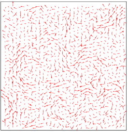
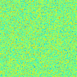
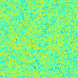
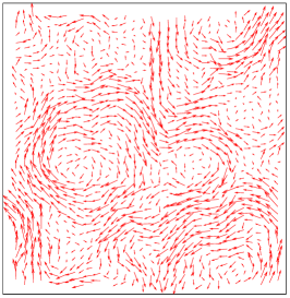
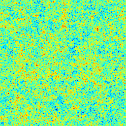
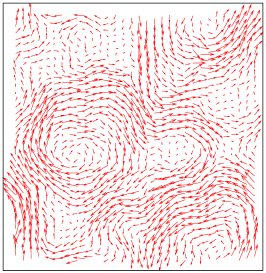
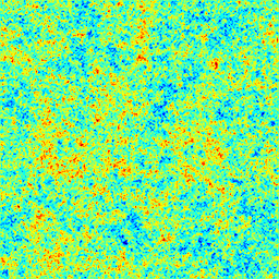
$H=0.01$       $H=\frac{1}{3}$       $H=\frac{1}{2}$       $H=\frac{2}{3}$       $H=1$      

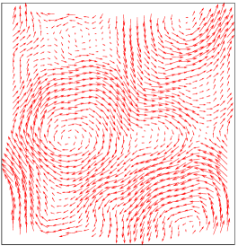
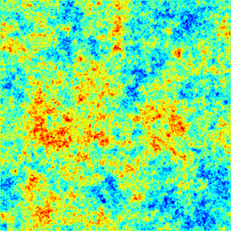
Fig. 1: Synthesized fBms $\mbox{$\mathbf{{u}}$}(\mathbf{x})=(u_{1}(\mathbf{x}),u_{2}(\mathbf{x}))^{T}$ for different values of $H$ (left). Associated vorticity maps, i.e. $\partial_{x}u_{2}(\mathbf{x})-\partial_{y}u_{1}(\mathbf{x})$ (right) .

In order to form an evaluation benchmark for the regularization model, a set of 5 fBm realizations were synthesized (from an identical white noise realization) with a resolution $2^{8}\times 2^{8}$ on the domain $[0,1]^{2}$. The wavelet generator was constructed from periodized Coiflets with 10 vanishing moments, so-called Coiflets-10 [33]. Note that these wavelets are 3 times differentiable so that our regularity assumptions are satisfied for any $H\leq 1$. The realizations are associated to Hurst exponents $H_{1}=0.01$, $H_{2}=\frac{1}{3}$, $H_{3}=\frac{1}{2}$, $H_{4}=\frac{2}{3}$ and $H_{5}=1$. Let us remark that the cases $H=\frac{1}{3}$ and $H=1$ are consistent with isotropic turbulence models introduced by Kolmogorov for 3D flows [27] (resp. by Kraichnan for 2D flows [28]), while the case $H=\frac{1}{2}$ constitutes a standard Brownian motion. Parameter $\sigma$ is chosen so that for any $\mathbf{x}$ belonging to the pixel grid, the displacement $|\mathbf{u}(\mathbf{x})|$ is not greater that $10\times 2^{-8}$, i.e. 10 pixels. Figure 1 displays vector fields $\mbox{$\mathbf{{u}}$}(\mathbf{x})=(u_{1}(\mathbf{x}),u_{2}(\mathbf{x}))^{t}$ and vorticity maps $\partial_{x}u_{2}(\mathbf{x})-\partial_{y}u_{1}(\mathbf{x})$ associated to the 5 fBms.

Let the radial power spectrum of $\mathbf{{u}}$ be defined by:

$$E(\kappa)\triangleq\int_{\mathcal{S}_{\kappa}}E_{1}(\mathbf{x})+E_{2}(\mathbf{x})d\mathbf{x},$$ (42)

where ${\mathcal{S}_{\kappa}}$ is the circle of radius $\kappa$. It is easy to check that according to (4), this function is $E(\kappa)=c\,\kappa^{-2H-1}$, where $c>0$. Therefore, the spectra of our 5 different fBms decay exponentially with power respectively equal to $-1.02$, $-\frac{5}{3}$, $-2$, $-\frac{7}{3}$ and $-3$.

6.2 Synthetic image couple generation

$H=\frac{1}{3}$
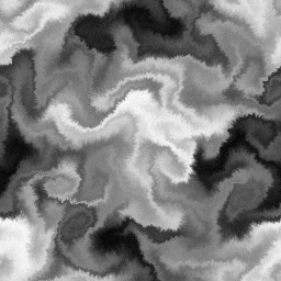
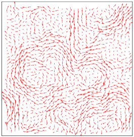
$H=1$

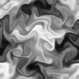
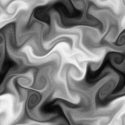
Fig. 2: Initial image $y_{0}$ (left), deformation field $\mathbf{{u}}$ (middle) and final image $y_{1}$ (right) for $H=\frac{1}{3}$ and $H=1$. Images $y_{0}$ and $y_{1}$ have been corrupted by a white noise.

To simulate the couple $(y_{0},y_{1})$ in the data-term (14), we start by a fixed image $y_{1}$ and derive $y_{0}$ from the relation $y_{0}(\mathbf{x})=y_{1}(\mathbf{x}+\mbox{$\mathbf{{u}}$}(\mathbf{x}))$ derived in section 4.1. Since $\mathbf{x}+\mbox{$\mathbf{{u}}$}(\mathbf{x})$ does not necessarily lie on the pixel grid, we used cubic B-splines for interpolation of $y_{1}$. To simulate realistic measurement conditions, the so-generated images were then corrupted by i.i.d. Gaussian noise yielding a peak signal to noise ratio (PSNR) on $y_{0}$ (resp. $y_{1}$) of 33.2 dB (resp. 33.5 dB). The resulting image pairs are displayed in figure 2 for $H=\frac{1}{3}$ and $H=1$.

6.3 Optic-flow evaluation procedure

The divergence-free fBm fields were estimated according to a MAP criterion, solving minimization problems (26) or (28). The proposed approaches are compared to two other standard regularizers, which all require the choice of a basis to decompose $\mathbf{{u}}$. In order to make relevant comparisons, we chose the divergence-free wavelet basis for all these alternatives. The wavelet generator was constructed from divergence-free biorthogonal Coiflets-10 with periodic boundary conditions. Moreover, the optimization procedure used for all regularizers was the same and relied on an identical data-term.

The five different estimation methods used for evaluation are listed and detailed hereafter. They are denoted A, B, C, D and E. Methods A and B are state-of-the-art algorithms while methods C, D and E implement the fBm prior.

• Penalization of $L^{2}$ norm of velocity components gradients. The most common approach in optic-flow estimation, as first proposed in [24], is to penalize the $L^{2}$ norm of the velocity gradients. We used the wavelet-based implementation proposed in [25].

• Penalization of $L^{2}$ norm of vorticity gradient. In fluid motion estimation a popular approach is to penalize the $L^{2}$ norm of the vorticity gradient [11, 45, 52]. Here again, we used the wavelet-based implementation proposed in [25].

• fBm regularization in a fractional Laplacian wavelet basis. This corresponds to solve (26) using algorithms 1 and 2.

• fBm regularization in a divergence-free wavelet basis. This corresponds to solve (28) computed without approximation using algorithms 3 and 4.

• Approached fBm regularization in a divergence-free wavelet basis. This corresponds to solve (28) where the regularization term is approached using algorithms 4 and 6.

Each of the regularizer in methods A, B, C, D and E were optimally tuned, that is to say regularization coefficient were chosen (using a brute-force approach) in order to the RMSE detailed hereafter. Note that an implicit regularization by polynomial approximation has also been tested. It is a well-known approach in computer vision [4, 13, 31, 50]. The performances were clearly below the previous approaches, so we do not display the results in this paper.

Let $\mathcal{S}$ denote the set of pixel sites. The two following criteria were used to evaluate the accuracy of estimated fields denoted by ${\mbox{$\mathbf{{u}}$}}^{*}$: the Root Mean Squared end-point Error (RMSE) in pixel

$$\text{RMSE}=\left(\frac{1}{n^{2}}\sum_{\mathbf{x}\in\mathcal{S}}\big{|}\mbox{$\mathbf{{u}}$}^{*}(\mathbf{x})-\mbox{$\mathbf{{u}}$}(\mathbf{x})\big{|}^{2}\right)^{\frac{1}{2}},$$

and the Mean Barron Angular Error (MBAE) in degrees

$$\text{MBAE}=\frac{1}{n^{2}}\sum_{\mathbf{x}\in\mathcal{S}}\text{arcos}\left(\frac{\mbox{$\mathbf{{u}}$}^{*}(\mathbf{x})\cdot\mbox{$\mathbf{{u}}$}(\mathbf{x})}{|\mbox{$\mathbf{{u}}$}{\rm}(\mathbf{x})|^{2}}\right),$$

where $\mathbf{{u}}$ represents the synthesized fBm. Moreover, we introduce a criterion to evaluate the accuracy of reconstruction of the power-law decay of the radial power spectrum. More precisely, in logarithmic coordinates the power-law (42) writes as an affine function of $\log(\kappa)$ of the form $-(2H+1)\log(\kappa)+\gamma$, depending on two parameters, namely the Hurst exponent $H$ and the intercept $\gamma$, that can be explicitly related to $\sigma$ in (4). Performing a linear regression (by the ordinary least squares method) on the estimated spectrum in logarithmic coordinates, we obtain an estimation of the affine function parameters denoted by $H^{*}$ and $\gamma^{*}$. The quality criterion is then chosen to be the $L^{1}$ distance between the estimated and true affine functions within the interval $[\log(\kappa_{min}),\log(\kappa_{max})]$ , called the Spectrum Absolute Error (SAE):

$$\text{SAE}=\int_{\log(\kappa_{min})}^{\log(\kappa_{max})}\!|2x(H-H^{*})+\gamma^{*}-\gamma|dx,$$

In order to evaluate the power-law reconstruction at small scales, we chose $\kappa_{min}=10$ and $\kappa_{max}=n$.

Finally, we performed an additional visual comparison of the accuracy of restituted vorticity maps.

6.4 Results

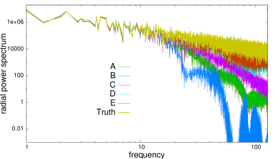
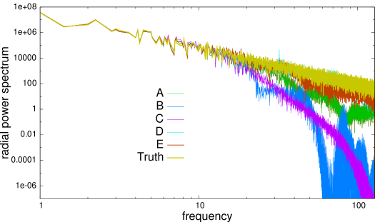
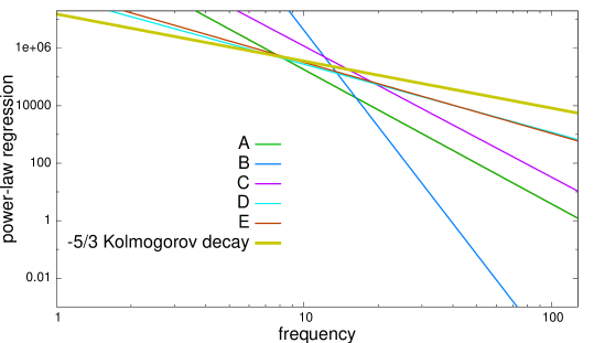
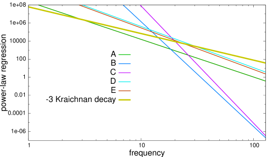
Fig. 4: Radial power spectrum estimates in logarithmic coordinates (above) and ordinary least squares fitting (below) for methods A to E (see section 6.3 for a description) for $H=\frac{1}{3}$ (left) and $H=1$ (right), compared to ground truth and the theoretical decay. Regularization coefficients where chosen to minimize the RMSE.

$H=\frac{1}{3}$
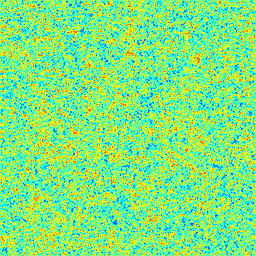
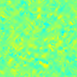
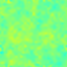
Truth	A	B
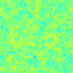
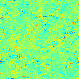
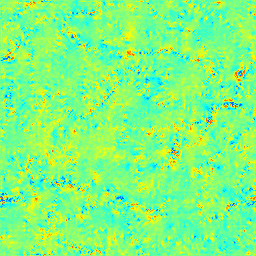
C	D	E
$H=1$
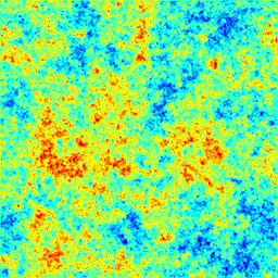
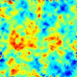
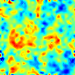
Truth	A	B
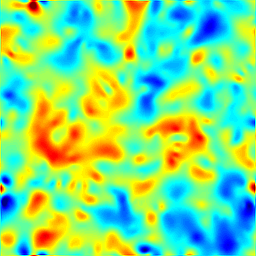
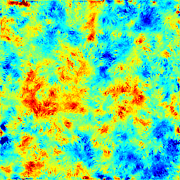
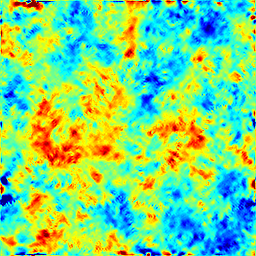
C	D	E

Fig. 5: Estimated vorticity maps for methods A to E (see section 6.3 for a description) and for $H=\frac{1}{3}$ (above) and $H=1$ (below). Regularization coefficients were chosen to minimize the RMSE

In table of figure 3, the performance of the proposed methods (C, D and E) can be compared in terms of RMSE, MBAE and SAE to state-of-the-art approaches (A and B). Let us comment these results. Methods C, D and E yield the best results with respect to each criterion. Method C, i.e. the method based on fractional Laplacian wavelets, provides the lowest RMSE and MBAE. An average RMSE gain of 19% with respect to the best state-of-the-art method is observed, with a peak at 26% for $H=\frac{1}{2}$. However, considering the 3 criteria jointly, methods D and E, i.e. exact and approached method based on divergence-free wavelets, provide the best compromise. In particular, according to SAE it can be noticed that, unlike method C, methods D and E achieve to accurately reconstruct the power-law decay of the fBm spectrum. This is illustrated in figure 4. Moreover, the approximation used to derive method E seems to be accurate since performance of E are very close to those of D. In figure 5, one can visualize estimated vorticity maps with the different methods for $H=\frac{1}{3}$ and $H=1$, i.e. fBms modeling respectively 3D or 2D turbulence. This figure clearly shows the superiority of methods D and E in reconstructing the fractal structure of the vorticity fields.

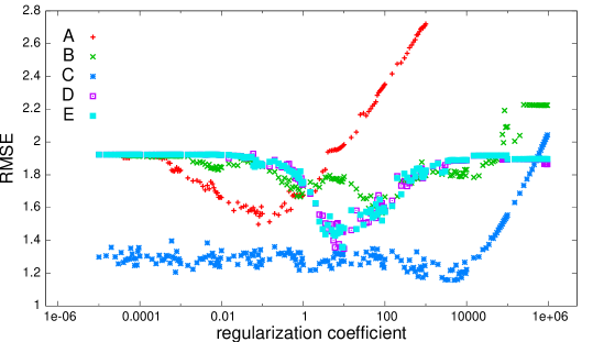
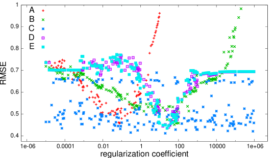
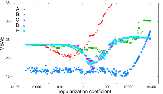
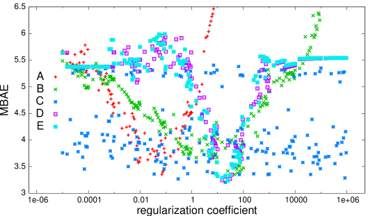
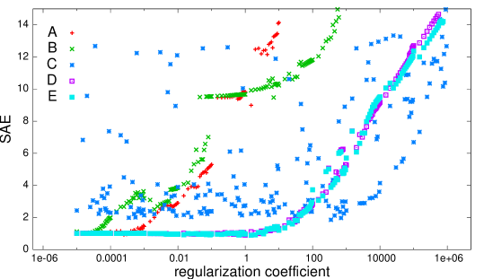
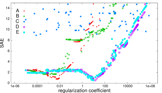
Fig. 6: Influence of regularization coefficient on the accuracy of the estimate in terms of RMSE (above), MBAE (middle) and SAE (below) for methods A to E (see section 6.3 for a description) and for $H=\frac{1}{3}$ (left) and $H=1$ (right).

$H=\frac{1}{3}$
Truth	A	B
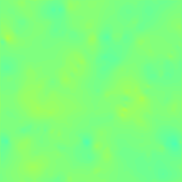
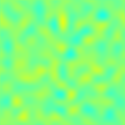
C	D	E
$H=1$
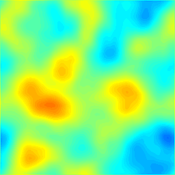
Truth	A	B
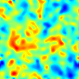
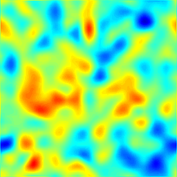
C	D	E

Fig. 7: Estimated vorticity maps for methods A to E (see section 6.3 for a description) for $H=\frac{1}{3}$ and $H=1$ in the case of a very large regularization coefficient $(\sim 1e6)$

Plots of figure 6 show the influence of the regularization parameter in terms of RMSE, MBAE and SAE for $H=\frac{1}{3}$ and $H=1$. Clear minima of RMSE and MBAE are visible for methods A, B, D and E. On the other hand, method C, i.e. fractional Laplacian wavelet basis, seems to be ‘unstable’ in the sense that it yields inhomogeneous performances for small variations of regularization parameter. The saturation of the RMSE and the MBAE for large values of the regularization parameter shows that, on the contrary to state-of-the-art methods, sensitivity of method D and E to the latter parameter is weak, in the sense that it yields reasonable estimation error even for regularization parameter far from an optimal value. This error saturation effect is illustrated in figure 7. It displays vorticity maps produced by the different methods for a very large regularization coefficient.

7 Conclusion

This work addresses the inverse-problem of estimating a hidden turbulent motion field from the observation of a pair of images. We adopt a Bayesian framework where we propose a family of divergence-free, isotropic, self-similar priors for this hidden field. Self-similarity and divergence-free are well known features of incompressible turbulence in statistical fluid mechanics. Our priors are bivariate fractional Brownian fields, resulting from the extra assumptions that the hidden field is Gaussian and has stationary increments. The main purpose of this article is the design of effective and efficient algorithms to achieve MAP estimation, by expanding these specific priors into well-chosen bases. From a spectral integral representation proved in Proposition 2, we represent divergence-free fBms in two specific wavelet bases. The first option (Proposition 3) is a fractional Laplacian wavelet basis which plays the role of a whitening filter in the sense that the wavelet coefficients are uncorrelated. The second alternative is to use a divergence-free wavelet basis, which is well-suited to our case. The latter wavelets simplify the decomposition, since they neither involve fractional operators nor Leray projector on the divergence-free functional space. However, the wavelets coefficients are then correlated. We provide a closed-form expression for the induced correlation structure (Proposition 4), which is necessary to implement this second approach in practice. For these two approaches, the algorithms to reach the MAP involve gradient based LBFGS optimization procedures and rely on fast transforms (FFT or/and FWT). Moreover we propose an approximation of the correlation structure of the coefficients in the divergence-free wavelets expansion. It is based on off-line computation of fractional Laplacian wavelet connection coefficients. This approximation leads to the fastest algorithm without loss of accuracy. According to an intensive numerical evaluation carried out in section 6, all proposed algorithms clearly outperform the state-of-the-art methods. Finally, in the light of our experiments, the divergence-free wavelet expansion seems to be the most appropriated representation to solve our MAP inverse-problem.

An obvious and important perspective is the assessment of the develops algorithms in the context of real turbulence. To simplify the exposition, this work essentially focuses on the bi-variate case, which is of interest in particular geophysical contexts. However, there may be some limitations in studying three-dimensional turbulence from bi-dimensional slices or projections of the flow [18]. Acquisition of three-dimensional data is not an easy task. In fact volume data is generally reconstructed from bi-dimensional information and this inverse problem still represents an active domain of research. Nevertheless, extension of our algorithms to the three-dimensional case is straightforward since no theoretical or technical issue constitute a block.

Appendix A Proofs

A.1 Proof of Proposition 2

Let us recall (see e.g. [51]) that given a standard Gaussian spectral measure $\tilde{W}_{1}$, the integral $\int f(\mathbf{k})\tilde{W}_{1}(d\mathbf{k})$ is well-defined whenever $f\in L^{2}(\mathbb{R}^{2})$, has zero expectation and for $f,g$ in $L^{2}(\mathbb{R}^{2})$:

$$\mathbb{E}\left(\int f(\mathbf{k})\tilde{W}_{1}(d\mathbf{k})\overline{\int g(\mathbf{k})\tilde{W}_{1}(d\mathbf{k})}\right)=\int f(\mathbf{k})\overline{g(\mathbf{k})}d\mathbf{k}.$$ (43)

In (2), the matrix ${\bf P}(\mathbf{k})\triangleq\left[\mathbf{I}-\frac{\mathbf{k}\mathbf{k}^{T}}{\|{\mathbf{k}}\|^{2}}\right]$ corresponds to the Leray projection matrix in the Fourier domain. It is easily verified that all entries of ${\bf P}$ are in $[0,1]$. For this reason the integral (2) is well defined, since for all $\mathbf{x}\in\mathbb{R}^{2}$ and all $H\in(0,1)$, the function $\mathbf{k}\mapsto(e^{i{\bf k}\cdot\mathbf{x}}-1)\|\mathbf{k}\|^{-H-1}$ belongs to $L^{2}(\mathbb{R}^{2})$.

Let us show that the structure function of $\mathbf{{u}}$ is given by (3). For $j=1,2$, denote ${\bf e}_{j}$ the bivariate vector whose $j$-th component is equal to one while the other component is zero. For all $i,j=1,2$, from (2) and (43), since ${\bf P}^{2}={\bf P}$, we get

$$\mathbb{E}[(\mbox{$\mathbf{{u}}$}_{i}(\mathbf{x}_{2})-\mbox{$\mathbf{{u}}$}_{i}(\mathbf{x}_{1}))\overline{(\mbox{$\mathbf{{u}}$}_{j}(\mathbf{x}_{4})-\mbox{$\mathbf{{u}}$}_{j}(\mathbf{x}_{3}))}]$$

$$=\frac{\sigma^{2}}{(2\pi)^{2}}\int_{\mathbb{R}^{2}}\ \|\mathbf{k}\|^{-2H-2}{\bf e}_{i}^{T}{\bf P}(\mathbf{k}){\bf e}_{j}\left(e^{i\mathbf{k}\cdot\mathbf{x}_{2}}-e^{i\mathbf{k}\cdot\mathbf{x}_{1}}\right)\left(e^{-i\mathbf{k}\cdot\mathbf{x}_{4}}-e^{-i\mathbf{k}\cdot\mathbf{x}_{3}}\right)d\mathbf{k}$$

$$=\frac{\sigma^{2}}{(2\pi)^{2}}\int_{\mathbb{R}^{2}}\ \|\mathbf{k}\|^{-2H-2}{\bf e}_{i}^{T}{\bf P}(\mathbf{k}){\bf e}_{j}\left(e^{i\mathbf{k}\cdot(\mathbf{x}_{2}-\mathbf{x}_{4})}-e^{i\mathbf{k}\cdot(\mathbf{x}_{2}-\mathbf{x}_{3})}-e^{i\mathbf{k}\cdot(\mathbf{x}_{1}-\mathbf{x}_{4})}+e^{i\mathbf{k}\cdot(\mathbf{x}_{1}-\mathbf{x}_{3})}\right)d\mathbf{k}.$$

We use Lemma 2.2 in [48] to get the following Fourier transform: for any $\mathbf{x}\in\mathbb{R}^{2}$

$$\frac{1}{(2\pi)^{2}}\int_{\mathbb{R}^{2}}\|\mathbf{k}\|^{-2H-2}{\bf P}(\mathbf{k})e^{i\mathbf{k}\cdot\mathbf{x}}d\mathbf{k}=c_{H}\|\mathbf{x}\|^{2H}\left(2H\frac{\mathbf{x}\mathbf{x}^{T}}{\|\mathbf{x}\|^{2}}-(2H+1)\mathbf{I}\right).$$

where $c_{H}={\Gamma(1-H)}/(\pi 2^{2H+2}\Gamma(H+1)H(2H+2))$. The structure function (3) is then deduced.

Finally (3) coincides with the structure function obtained in [48] Section 4.5 when $\mathbf{{u}}$ is defined by (1). As this structure function characterizes the law of the Gaussian vector field $\mathbf{{u}}$, this shows that the two vector fields defined by (2) and (1) share the same distribution.

$\square$

A.2 Proof of Proposition 3

Let us denote by $\Phi_{0}$ the indicator function $\mathbb{I}_{[0,1]^{2}}(\mathbf{x})$, so that according to the construction explained in Section 3.1, the wavelets $\Phi_{{\boldsymbol{\ell}},{\boldsymbol{s}}}$, for $({\boldsymbol{\ell}},{\boldsymbol{s}})\in\Omega\cup 0$, form an orthonormal basis of $L^{2}([0,1]^{2})$. For any function $\mbox{$\mathbf{{v}}$}\in L^{2}([0,1]^{2})$, we have $\mbox{$\mathbf{{v}}$}(\mathbf{x})=\sum_{({\boldsymbol{\ell}},{\boldsymbol{s}})\in\Omega\cup 0}\langle\mbox{$\mathbf{{v}}$},{\Phi}_{{\boldsymbol{\ell}},{\boldsymbol{s}}}\rangle\Phi_{{\boldsymbol{\ell}},{\boldsymbol{s}}}(\mathbf{x})$ in $L^{2}([0,1]^{2})$, where $\langle.,.\rangle$ denotes the scalar product in $L^{2}([0,1]^{2})$. The same relation holds in $L^{2}(\mathbb{R}^{2})$ if each function is extended outside $[0,1]^{2}$ by zero, and we denote these extensions $\mbox{$\mathbf{{v}}$}^{0}$ and ${\Phi}^{0}_{{\boldsymbol{\ell}},{\boldsymbol{s}}}$ respectively. Hence, by the Plancherel’s theorem, we deduce that $\mathcal{F}\mbox{$\mathbf{{v}}$}^{0}({\bf k})=\sum_{\ell,{\boldsymbol{s}}}\langle\mathcal{F}\mbox{$\mathbf{{v}}$}^{0},\mathcal{F}{\Phi}^{0}_{{\boldsymbol{\ell}},{\boldsymbol{s}}}\rangle\mathcal{F}{\Phi}^{0}_{{\boldsymbol{\ell}},{\boldsymbol{s}}}({\bf k})$ in $L^{2}(\mathbb{R}^{2})$, where now $\langle.,.\rangle$ denotes the scalar product in $L^{2}(\mathbb{R}^{2})$. Therefore, for $j=1,2$,

$$\int_{\mathbb{R}^{2}}\mathcal{F}\mbox{$\mathbf{{v}}$}^{0}({\bf k})\tilde{W}_{j}(d{\bf k}) =\sum_{\ell,{\boldsymbol{s}}}\langle\mathcal{F}\mbox{$\mathbf{{v}}$}^{0},\mathcal{F}{\Phi}^{0}_{{\boldsymbol{\ell}},{\boldsymbol{s}}}\rangle\eta^{j}_{{\boldsymbol{\ell}},{\boldsymbol{s}}}$$ (44)

with

$$\eta^{j}_{{\boldsymbol{\ell}},{\boldsymbol{s}}}=\int_{\mathbb{R}^{2}}\mathcal{F}{\Phi}^{0}_{{\boldsymbol{\ell}},{\boldsymbol{s}}}({\bf k})\tilde{W}_{j}(d{\bf k}).$$ (45)

From (43) and the Plancherel’s theorem, since the wavelets are orthogonal and normalized in $L^{2}$, we note that $\eta^{j}_{{\boldsymbol{\ell}},{\boldsymbol{s}}}$ are i.i.d standard Gaussian random variables.

Now recall from (2) that $\mbox{$\mathbf{{u}}$}(\mathbf{x})=(\mbox{$\mathbf{{u}}$}_{1}(\mathbf{x}),\mbox{$\mathbf{{u}}$}_{2}(\mathbf{x}))^{T}$ where for $i=1,2$, $\mbox{$\mathbf{{u}}$}_{i}(\mathbf{x})=\int\mathcal{F}\mbox{$\mathbf{{v}}$}^{0}_{i1}(\mathbf{k})\tilde{W}_{1}(d\mathbf{k})+\int\mathcal{F}\mbox{$\mathbf{{v}}$}^{0}_{i2}(\mathbf{k})\tilde{W}_{2}(d\mathbf{k})$ with

$$\mathcal{F}\mbox{$\mathbf{{v}}$}^{0}_{ij}(\mathbf{k})=\frac{\sigma}{2\pi}\,(e^{i{\bf k}\cdot\mathbf{x}}-1)\|\mathbf{k}\|^{-H-1}(\delta_{ij}-{k}_{i}{k}_{j}/\|{\bf k\|^{2}}).$$ (46)

Applying (44) to $\mbox{$\mathbf{{v}}$}=\mbox{$\mathbf{{v}}$}_{i1},\mbox{$\mathbf{{v}}$}_{i2},$ we obtain for $i=1,2$

$$\mbox{$\mathbf{{u}}$}_{i}(\mathbf{x}) =\sum_{({\boldsymbol{\ell}},{\boldsymbol{s}})\in\Omega\cup 0,\,j\in\{1,2\}}\eta^{j}_{{\boldsymbol{\ell}},{\boldsymbol{s}}}\langle\mathcal{F}\mbox{$\mathbf{{v}}$}^{0}_{ij},\mathcal{F}{\Phi}^{0}_{{\boldsymbol{\ell}},{\boldsymbol{s}}}\rangle$$

$$=\sum_{({\boldsymbol{\ell}},{\boldsymbol{s}})\in\Omega\cup 0,\,j\in\{1,2\}}\eta^{j}_{{\boldsymbol{\ell}},{\boldsymbol{s}}}\int_{\mathbb{R}^{2}}\mathcal{F}\mbox{$\mathbf{{v}}$}^{0}_{ij}(\mathbf{k})\mathcal{F}{\Phi}^{0}_{{\boldsymbol{\ell}},{\boldsymbol{s}}}(\mathbf{k})d\mathbf{k},$$

and from (46) we deduce the representation

$$\mbox{$\mathbf{{u}}$}(\mathbf{x}) =\frac{\sigma}{2\pi}\sum_{({\boldsymbol{\ell}},{\boldsymbol{s}})\in\Omega\cup 0}\int_{\mathbb{R}^{2}}(e^{i{\bf k}\cdot\mathbf{x}}-1)\left[\mathbf{I}-\frac{\mathbf{k}\mathbf{k}^{T}}{\|{\mathbf{k}}\|^{2}}\right]\boldsymbol{\eta}_{{\boldsymbol{\ell}},{\boldsymbol{s}}}\|\mathbf{k}\|^{-H-1}\mathcal{F}{\Phi}^{0}_{{\boldsymbol{\ell}},{\boldsymbol{s}}}({\bf k})d{\bf k},$$ (47)

where $\boldsymbol{\eta}_{{\boldsymbol{\ell}},{\boldsymbol{s}}}\triangleq(\eta^{1}_{{\boldsymbol{\ell}},{\boldsymbol{s}}},\eta^{2}_{{\boldsymbol{\ell}},{\boldsymbol{s}}})^{T}$.

Since the mother wavelet $\psi$ has $M$ vanishing moments, for any $({\boldsymbol{\ell}},{\boldsymbol{s}})\in\Omega$, $\Phi_{{\boldsymbol{\ell}},{\boldsymbol{s}}}$ has $M$ vanishing moments along at least one direction (say $\mathbf{x}_{1}$). As a consequence, there exists a bounded function ${\theta}_{{\boldsymbol{\ell}},{\boldsymbol{s}}}$ such that $\mathcal{F}{\Phi}^{0}_{{\boldsymbol{\ell}},{\boldsymbol{s}}}(\mathbf{k})=(-ik_{1})^{M}{\theta}_{{\boldsymbol{\ell}},{\boldsymbol{s}}}(\mathbf{k})$ (see [33]). So $|\|\mathbf{k}\|^{-H-1}\mathcal{F}{\Phi}^{0}_{{\boldsymbol{\ell}},{\boldsymbol{s}}}({\bf k})|=|\|\mathbf{k}\|^{-H-1}(-ik_{1})^{M}{\theta}_{{\boldsymbol{\ell}},{\boldsymbol{s}}}(\mathbf{k})|\leq c\|\mathbf{k}\|^{M-H-1}$, where $c$ is some positive constant. Since $M>H$, the latter bound shows that $\mathbf{k}\mapsto\|\mathbf{k}\|^{-H-1}\mathcal{F}{\Phi}^{0}_{{\boldsymbol{\ell}},{\boldsymbol{s}}}({\bf k})$ is square-integrable on any compact. Moreover it is square-integrable at infinity as $\mathbf{k}\mapsto\mathcal{F}{\Phi}^{0}_{{\boldsymbol{\ell}},{\boldsymbol{s}}}({\bf k})$ is, while $\mathbf{k}\mapsto\|\mathbf{k}\|^{-H-1}$ asymptotically vanishes. Hence, for any $({\boldsymbol{\ell}},{\boldsymbol{s}})\in\Omega$, $\mathbf{k}\mapsto\|\mathbf{k}\|^{-H-1}\mathcal{F}{\Phi}^{0}_{{\boldsymbol{\ell}},{\boldsymbol{s}}}({\bf k})\in L^{2}(\mathbb{R}^{2})$ and the integral in (47) can be split, leading to the representation in $(L^{2}([0,1]^{2}))^{2}$,

$$\mbox{$\mathbf{{u}}$}(\mathbf{x})=2\pi\sigma\sum_{({\boldsymbol{\ell}},{\boldsymbol{s}})\in\Omega}\, \mathcal{P}\left[\boldsymbol{\eta}_{{\boldsymbol{\ell}},{\boldsymbol{s}}}{\Phi}^{(-H-1)}_{{\boldsymbol{\ell}},{\boldsymbol{s}}}\right]({\mathbf{x}})-\mathcal{P}\left[\boldsymbol{\eta}_{{\boldsymbol{\ell}},{\boldsymbol{s}}}{\Phi}^{(-H-1)}_{{\boldsymbol{\ell}},{\boldsymbol{s}}}\right](0)$$

$$+\frac{\sigma}{2\pi}\int_{\mathbb{R}^{2}}(e^{i{\bf k}\cdot\mathbf{x}}-1)\left[\mathbf{I}-\frac{\mathbf{k}\mathbf{k}^{T}}{\|{\mathbf{k}}\|^{2}}\right]\boldsymbol{\eta}_{0}\|\mathbf{k}\|^{-H-1}\mathcal{F}{\Phi}^{0}_{0}({\bf k})d{\bf k},$$ (48)

where ${\Phi}^{(-H-1)}_{{\boldsymbol{\ell}},{\boldsymbol{s}}}$ and $\mathcal{P}$ are respectively defined in (8) and (9), and $\boldsymbol{\eta}_{{\boldsymbol{\ell}},{\boldsymbol{s}}}{\Phi}^{(-H-1)}_{{\boldsymbol{\ell}},{\boldsymbol{s}}}$ is the bivariate vector $(\eta^{1}_{{\boldsymbol{\ell}},{\boldsymbol{s}}}{\Phi}^{(-H-1)}_{{\boldsymbol{\ell}},{\boldsymbol{s}}},\eta^{2}_{{\boldsymbol{\ell}},{\boldsymbol{s}}}{\Phi}^{(-H-1)}_{{\boldsymbol{\ell}},{\boldsymbol{s}}})^{T}$.

The decomposition (10) is a consequence of (A.2), where $\boldsymbol{\epsilon}_{{\boldsymbol{\ell}},{\boldsymbol{s}}}\triangleq 2\pi\sigma\boldsymbol{\eta}_{{\boldsymbol{\ell}},{\boldsymbol{s}}}$, provided we prove that

$$\sum_{({\boldsymbol{\ell}},{\boldsymbol{s}})\in\Omega}\mathcal{P}\left[\boldsymbol{\eta}_{{\boldsymbol{\ell}},{\boldsymbol{s}}}{\Phi}^{(-H-1)}_{{\boldsymbol{\ell}},{\boldsymbol{s}}}\right](0)=\frac{1}{(2\pi)^{2}}\int_{\mathbb{R}^{2}}(e^{i{\bf k}\cdot\mathbf{x}}-1)\left[\mathbf{I}-\frac{\mathbf{k}\mathbf{k}^{T}}{\|{\mathbf{k}}\|^{2}}\right]\boldsymbol{\eta}_{0}\|\mathbf{k}\|^{-H-1}\mathcal{F}{\Phi}^{0}_{0}({\bf k})d{\bf k}.$$ (49)

Since by assumption $\int_{[0,1]^{2}}\mbox{$\mathbf{{u}}$}(\mathbf{x})d\mathbf{x}=0$, integrating both sides of (A.2) on $[0,1]^{2}$ leads to

$$\sum_{({\boldsymbol{\ell}},{\boldsymbol{s}})\in\Omega}\int_{[0,1]^{2}}\mathcal{P}\left[\boldsymbol{\eta}_{{\boldsymbol{\ell}},{\boldsymbol{s}}}{\Phi}^{(-H-1)}_{{\boldsymbol{\ell}},{\boldsymbol{s}}}\right]({\mathbf{x}})d\mathbf{x}-\mathcal{P}\left[\boldsymbol{\eta}_{{\boldsymbol{\ell}},{\boldsymbol{s}}}{\Phi}^{(-H-1)}_{{\boldsymbol{\ell}},{\boldsymbol{s}}}\right](0)$$

$$+\frac{1}{(2\pi)^{2}}\int_{[0,1]^{2}}d\mathbf{x}\int_{\mathbb{R}^{2}}(e^{i{\bf k}\cdot\mathbf{x}}-1)\left[\mathbf{I}-\frac{\mathbf{k}\mathbf{k}^{T}}{\|{\mathbf{k}}\|^{2}}\right]\boldsymbol{\eta}_{0}\|\mathbf{k}\|^{-H-1}\mathcal{F}{\Phi}^{0}_{0}({\bf k})d{\bf k}=0.$$ (50)

Let $\boldsymbol{z}(\mathbf{x})=\boldsymbol{\eta}_{{\boldsymbol{\ell}},{\boldsymbol{s}}}{\Phi}^{(-H-1)}_{{\boldsymbol{\ell}},{\boldsymbol{s}}}({\mathbf{x}})$. Since wavelets possess at least one vanishing moment $\int_{[0,1]^{2}}\boldsymbol{z}({\mathbf{x}})d\mathbf{x}=0$. According to Definition (9) of the Leray projector this implies that $\int_{[0,1]^{2}}\mathcal{P}\boldsymbol{z}(\mathbf{x})d\mathbf{x}=0$ and therefore

$$\sum_{({\boldsymbol{\ell}},{\boldsymbol{s}})\in\Omega}\int_{[0,1]^{2}}\mathcal{P}\left[\boldsymbol{\eta}_{{\boldsymbol{\ell}},{\boldsymbol{s}}}{\Phi}^{(-H-1)}_{{\boldsymbol{\ell}},{\boldsymbol{s}}}\right]({\mathbf{x}})d\mathbf{x}=0.$$ (51)

Now consider the last term in (A.2). We have for $j=1,2$

$$\frac{\partial}{\partial x_{j}}\int_{\mathbb{R}^{2}}(e^{i{\bf k}\cdot\mathbf{x}}-1)\left[\mathbf{I}-\frac{\mathbf{k}\mathbf{k}^{T}}{\|{\mathbf{k}}\|^{2}}\right]\boldsymbol{\eta}_{0}\|\mathbf{k}\|^{-H-1}\mathcal{F}{\Phi}^{0}_{0}({\bf k})d{\bf k}$$

$$=\int_{\mathbb{R}^{2}}(ik_{j})e^{i{\bf k}\cdot\mathbf{x}}\left[\mathbf{I}-\frac{\mathbf{k}\mathbf{k}^{T}}{\|{\mathbf{k}}\|^{2}}\right]\boldsymbol{\eta}_{0}\|\mathbf{k}\|^{-H-1}\mathcal{F}{\Phi}^{0}_{0}({\bf k})d{\bf k}$$

$$=\int_{\mathbb{R}^{2}}e^{i{\bf k}\cdot\mathbf{x}}\left[\mathbf{I}-\frac{\mathbf{k}\mathbf{k}^{T}}{\|{\mathbf{k}}\|^{2}}\right]\boldsymbol{\eta}_{0}\|\mathbf{k}\|^{-H-1}\left(\int_{\mathbb{R}^{2}}e^{-i\mathbf{k}\cdot\mathbf{x}}\frac{\partial}{\partial x_{j}}\mathbb{I}_{[0,1]^{2}}({\mathbf{x}})d\mathbf{x}\right)d{\bf k}=0.$$

Therefore, we obtain

$$\int_{[0,1]^{2}}d\mathbf{x}\int_{\mathbb{R}^{2}}(e^{i{\bf k}\cdot\mathbf{x}}-1)\left[\mathbf{I}-\frac{\mathbf{k}\mathbf{k}^{T}}{\|{\mathbf{k}}\|^{2}}\right]\boldsymbol{\eta}_{0}\|\mathbf{k}\|^{-H-1}\mathcal{F}{\Phi}^{0}_{0}({\bf k})d{\bf k}$$

$$=\int_{\mathbb{R}^{2}}(e^{i{\bf k}\cdot\mathbf{x}}-1)\left[\mathbf{I}-\frac{\mathbf{k}\mathbf{k}^{T}}{\|{\mathbf{k}}\|^{2}}\right]\boldsymbol{\eta}_{0}\|\mathbf{k}\|^{-H-1}\mathcal{F}{\Phi}^{0}_{0}({\bf k})d{\bf k}.$$ (52)

Using (51) and (A.2) in (A.2) proves (49), which concludes the proof.

$\square$

A.3 Proof of Proposition 4

From (10), we have

$$d_{{\boldsymbol{\ell}},{\bf s}} =\sum_{({\bf i},{\bf j})\in\Omega}\langle\mathcal{P}\left[\boldsymbol{\epsilon}_{({\bf i},{\bf j})}{\Phi}^{(-H-1)}_{({\bf i},{\bf j})}\right]/\tilde{\boldsymbol{\Psi}}_{{\boldsymbol{\ell}},{\bf s}}\rangle=\sum_{({\bf i},{\bf j})\in{\Omega}}\langle\boldsymbol{\epsilon}_{({\bf i},{\bf j})}{\Phi}^{(-H-1)}_{({\bf i},{\bf j})}/\mathcal{P}\left[\tilde{\boldsymbol{\Psi}}_{{\boldsymbol{\ell}},{\bf s}}\right]\rangle,$$

where the scalar product is in $(L^{2}([0,1]^{2}))^{2}$. In the above formula and in the following, $\tilde{\boldsymbol{\Psi}}_{{\boldsymbol{\ell}},{\bf s}}$ is extended outside $[0,1]^{2}$ by zero, so that the operation $\mathcal{P}\left[\tilde{\boldsymbol{\Psi}}_{{\boldsymbol{\ell}},{\bf s}}\right]$ makes sense according to Definition (9). In other words, the definition of $\tilde{\boldsymbol{\Psi}}_{{\boldsymbol{\ell}},{\bf s}}$ in Section 3.2 becomes in this case $\mathcal{F}\tilde{\boldsymbol{\Psi}}_{{\boldsymbol{\ell}},{\bf s}}=(-1/(ik_{2})\mathcal{F}\Phi^{0}_{{\boldsymbol{\ell}},{\bf s}}(\mathbf{k}),(1/ik_{1})\mathcal{F}\Phi^{0}_{{\boldsymbol{\ell}},{\bf s}}(\mathbf{k}))^{T}$.

Since $\boldsymbol{\epsilon}_{({\bf i},{\bf j})}$ are iid zero-mean Gaussian random variables with variance $(2\pi\sigma)^{2}\bf I$, we have

$${(2\pi\sigma)^{-2}}\mathbb{E}[d_{{\boldsymbol{\ell}},{\bf s}}d_{{\boldsymbol{\ell}}^{\prime},{\bf s}^{\prime}}]=\\ \sum_{({\bf i},{\bf j})\in\Omega}\langle\Phi^{(-H-1)}_{{\bf i},{\bf j}},\mathcal{P}^{1}\tilde{\boldsymbol{\Psi}}_{{\boldsymbol{\ell}},{\bf s}}\rangle\langle\Phi^{(-H-1)}_{{\bf i},{\bf j}},\mathcal{P}^{1}\tilde{\boldsymbol{\Psi}}_{{\boldsymbol{\ell}}^{\prime},{\bf s}^{\prime}}\rangle+\langle\Phi^{(-H-1)}_{{\bf i},{\bf j}},\mathcal{P}^{2}\tilde{\boldsymbol{\Psi}}_{{\boldsymbol{\ell}},{\bf s}}\rangle\langle\Phi^{(-H-1)}_{{\bf i},{\bf j}},\mathcal{P}^{2}\tilde{\boldsymbol{\Psi}}_{{\boldsymbol{\ell}}^{\prime},{\bf s}^{\prime}}\rangle,$$

where $\mathcal{P}^{k}$ is the $k$-th row of matrix operator $\mathcal{P}$, i.e. given in the Fourier domain by $\mathcal{F}\mathcal{P}^{1}=(1-k_{1}^{2}/\|\mathbf{k}\|^{2},-k_{1}k_{2}/\|\mathbf{k}\|^{2})$ and $\mathcal{F}\mathcal{P}^{2}=(-k_{1}k_{2}/\|\mathbf{k}\|^{2},1-k_{2}^{2}/\|\mathbf{k}\|^{2})$.

Let us simplify the sum above. First, recall that ${\Phi}^{(-H-1)}_{{\boldsymbol{\ell}},{\bf s}}(\mathbf{x})={(-\Delta)^{\frac{-H-1}{2}}{\Phi}^{0}_{{\boldsymbol{\ell}},{\bf s}}}({\mathbf{x}})$, so for any $k=1,2$:

$$\sum_{({\bf i},{\bf j})\in\Omega}\langle\Phi^{(-H-1)}_{{\bf i},{\bf j}},\mathcal{P}^{k}\tilde{\boldsymbol{\Psi}}_{{\boldsymbol{\ell}},{\bf s}}\rangle \langle\Phi^{(-H-1)}_{{\bf i},{\bf j}},\mathcal{P}^{k}\tilde{\boldsymbol{\Psi}}_{{\boldsymbol{\ell}}^{\prime},{\bf s}^{\prime}}\rangle$$

$$=\langle\sum_{({\bf i},{\bf j})\in\Omega}\Phi^{(-H-1)}_{{\bf i},{\bf j}}\langle\Phi^{(-H-1)}_{{\bf i},{\bf j}},\mathcal{P}^{k}\tilde{\boldsymbol{\Psi}}_{{\boldsymbol{\ell}}^{\prime},{\bf s}^{\prime}}\rangle,\mathcal{P}^{k}\tilde{\boldsymbol{\Psi}}_{{\boldsymbol{\ell}},{\bf s}}\rangle$$

$$=\langle\sum_{({\bf i},{\bf j})\in\Omega}\Phi^{0}_{{\bf i},{\bf j}}\langle\Phi^{0}_{{\bf i},{\bf j}},(-\Delta)^{\frac{-H-1}{2}}\mathcal{P}^{k}\tilde{\boldsymbol{\Psi}}_{{\boldsymbol{\ell}}^{\prime},{\bf s}^{\prime}}\rangle,(-\Delta)^{\frac{-H-1}{2}}\mathcal{P}^{k}\tilde{\boldsymbol{\Psi}}_{{\boldsymbol{\ell}},{\bf s}}\rangle.$$

Since the mother wavelet $\psi$ has $M>H$ vanishing moments, similar arguments as in the proof of Proposition 3 lead to $|\|\mathbf{k}\|^{-H-1}\mathcal{F}[\mathcal{P}^{k}{\tilde{\boldsymbol{\Psi}}}_{{\boldsymbol{\ell}^{\prime}},{\bf s}^{\prime}}](\mathbf{k})|\leq c\|\mathbf{k}\|^{M-H-1}$, where $c$ is some positive constant. So

$$\int_{[0,1]^{2}}(-\Delta)^{\frac{-H-1}{2}}\mathcal{P}^{k}\tilde{\boldsymbol{\Psi}}_{{\boldsymbol{\ell}}^{\prime},{\bf s}^{\prime}}(\mathbf{x})d\mathbf{x}=\|\mathbf{k}\|^{-H-1}\mathcal{F}[\mathcal{P}^{k}{\tilde{\boldsymbol{\Psi}}}_{{\boldsymbol{\ell}^{\prime}},{\bf s}^{\prime}}](\mathbf{k})\Big{|}_{\mathbf{k}=0}=0$$

and we have the equality in $L^{2}([0,1]^{2})$ :

$$\sum_{({\bf i},{\bf j})\in\Omega}\Phi_{{\bf i},{\bf j}}\langle\Phi^{0}_{{\bf i},{\bf j}},(-\Delta)^{\frac{-H-1}{2}}\mathcal{P}^{k}\tilde{\boldsymbol{\Psi}}_{{\boldsymbol{\ell}}^{\prime},{\bf s}^{\prime}}\rangle =\sum_{({\bf i},{\bf j})\in\Omega\cup 0}\Phi_{{\bf i},{\bf j}}\langle\Phi^{0}_{{\bf i},{\bf j}},(-\Delta)^{\frac{-H-1}{2}}\mathcal{P}^{k}\tilde{\boldsymbol{\Psi}}_{{\boldsymbol{\ell}}^{\prime},{\bf s}^{\prime}}\rangle$$

$$=(-\Delta)^{\frac{-H-1}{2}}\mathcal{P}^{k}\tilde{\boldsymbol{\Psi}}_{{\boldsymbol{\ell}}^{\prime},{\bf s}^{\prime}}.$$

Therefore

$$\sum_{({\bf i},{\bf j})\in\Omega}\langle\Phi^{(-H-1)}_{{\bf i},{\bf j}},\mathcal{P}^{k}\tilde{\boldsymbol{\Psi}}_{{\boldsymbol{\ell}},{\bf s}}\rangle\langle\Phi^{(-H-1)}_{{\bf i},{\bf j}},\mathcal{P}^{k}\tilde{\boldsymbol{\Psi}}_{{\boldsymbol{\ell}}^{\prime},{\bf s}^{\prime}}\rangle =\langle(-\Delta)^{\frac{-H-1}{2}}\mathcal{P}^{k}\tilde{\boldsymbol{\Psi}}_{{\boldsymbol{\ell}}^{\prime},{\bf s}^{\prime}},\,(-\Delta)^{\frac{-H-1}{2}}\mathcal{P}^{k}\tilde{\boldsymbol{\Psi}}_{{\boldsymbol{\ell}},{\bf s}}\rangle$$

and

$$\mathbb{E}[d_{{\boldsymbol{\ell}},{\bf s}}d_{{\boldsymbol{\ell}}^{\prime},{\bf s}^{\prime}}]={(2\pi\sigma)^{2}}\langle(-\Delta)^{\frac{-H-1}{2}}\mathcal{P}\tilde{\boldsymbol{\Psi}}_{{\boldsymbol{\ell}},{\bf s}}/\,(-\Delta)^{\frac{-H-1}{2}}\mathcal{P}\tilde{\boldsymbol{\Psi}}_{{\boldsymbol{\ell}}^{\prime},{\bf s}^{\prime}}\rangle.$$ (53)

Since the operators $\mathcal{P}$ and $(-\Delta)^{\frac{-H-1}{2}}$ commute, and $\mathcal{P}$ is self-adjoint with $\mathcal{P}\mathcal{P}=\mathcal{P}$, we have

$$\mathbb{E}[d_{{\boldsymbol{\ell}},{\bf s}}d_{{\boldsymbol{\ell}}^{\prime},{\bf s}^{\prime}}]={(2\pi\sigma)^{2}}\langle(-\Delta)^{\frac{-H-1}{2}}\mathcal{P}\tilde{\boldsymbol{\Psi}}_{{\boldsymbol{\ell}},{\bf s}}/\,(-\Delta)^{\frac{-H-1}{2}}\tilde{\boldsymbol{\Psi}}_{{\boldsymbol{\ell}}^{\prime},{\bf s}^{\prime}}\rangle,$$

that is by Parseval relation

$$\mathbb{E}[d_{{\boldsymbol{\ell}},{\bf s}} d_{{\boldsymbol{\ell}}^{\prime},{\bf s}^{\prime}}]$$

$$={(2\pi\sigma)^{2}}\langle\|\mathbf{k}\|^{-H-1}\left[\mathbf{I}-\frac{\mathbf{k}\mathbf{k}^{T}}{\|{\mathbf{k}}\|^{2}}\right]\binom{-\frac{1}{ik_{2}}\mathcal{F}\Phi^{0}_{{\boldsymbol{\ell}},{\bf s}}(\mathbf{k})}{\frac{1}{ik_{1}}\mathcal{F}\Phi^{0}_{{\boldsymbol{\ell}},{\bf s}}(\mathbf{k})}/\,\|\mathbf{k}\|^{-H-1}\binom{-\frac{1}{ik_{2}}\mathcal{F}\Phi^{0}_{{\boldsymbol{\ell}},{\bf s}}(\mathbf{k})}{\frac{1}{ik_{1}}\mathcal{F}\Phi^{0}_{{\boldsymbol{\ell}},{\bf s}}(\mathbf{k})}\rangle$$

$$={(2\pi\sigma)^{2}}\langle\|\mathbf{k}\|^{-2H-2}\left(\frac{k_{2}^{2}}{\|\mathbf{k}\|^{2}}\frac{1}{k_{2}}+\frac{k_{1}k_{2}}{\|\mathbf{k}\|^{2}}\frac{1}{k_{1}}\right)\frac{1}{k_{2}}\mathcal{F}\Phi^{0}_{{\boldsymbol{\ell}},{\bf s}}(\mathbf{k}),\mathcal{F}\Phi^{0}_{{\boldsymbol{\ell}},{\bf s}}(\mathbf{k})\rangle$$

$$\qquad+{(2\pi\sigma)^{2}}\langle\|\mathbf{k}\|^{-2H-2}\left(\frac{k_{1}k_{2}}{\|\mathbf{k}\|^{2}}\frac{1}{k_{2}}+\frac{k_{1}^{2}}{\|\mathbf{k}\|^{2}}\frac{1}{k_{1}}\right)\frac{1}{k_{1}}\mathcal{F}\Phi^{0}_{{\boldsymbol{\ell}},{\bf s}}(\mathbf{k}),\mathcal{F}\Phi^{0}_{{\boldsymbol{\ell}},{\bf s}}(\mathbf{k})\rangle$$

$$={(2\pi\sigma)^{2}}\langle 4\|\mathbf{k}\|^{-2H-4}\mathcal{F}\Phi^{0}_{{\boldsymbol{\ell}},{\bf s}}(\mathbf{k}),\mathcal{F}\Phi^{0}_{{\boldsymbol{\ell}},{\bf s}}(\mathbf{k})\rangle.$$

$$=4{(2\pi\sigma)^{2}}\langle{\Phi}^{(-H-2)}_{{\boldsymbol{\ell}},{\bf s}},{\Phi}^{(-H-2)}_{{\boldsymbol{\ell}^{\prime}},{\bf s^{\prime}}}\rangle,$$

where the existence of wavelet ${\Phi}^{(-H-2)}_{{\boldsymbol{\ell}},{\bf s}}$ is guaranteed by the $M>H$ vanishing moments of the mother wavelet $\psi$.

$\square$

A.4 Proof of Lemma 5

When $n\to\infty$, the matrix ${\bf\Sigma}_{n}$ becomes the operator $\underline{\boldsymbol{\Sigma}}:\ell^{2}(\Omega)\rightarrow\ell^{2}(\Omega)$ defined for any $a\in\ell^{2}(\Omega)$ by:

$$[\underline{\boldsymbol{\Sigma}}a]_{{\boldsymbol{\ell}},{\boldsymbol{s}}} \triangleq\sum_{({\boldsymbol{\ell}}^{\prime},{\boldsymbol{s}}^{\prime})\in\Omega}a_{{\boldsymbol{\ell}}^{\prime},{\boldsymbol{s}}^{\prime}}{\Sigma}({{\boldsymbol{\ell}},{\boldsymbol{s}}},{\boldsymbol{\ell}}^{\prime},{\boldsymbol{s}}^{\prime}),\hskip 8.5359pt\forall({\boldsymbol{\ell}},{\boldsymbol{s}})\in\Omega,$$ (54)

where ${\Sigma}({{\boldsymbol{\ell}},{\boldsymbol{s}}},{\boldsymbol{\ell}}^{\prime},{\boldsymbol{s}}^{\prime})$ is given by (4.2). Similarly, the matrix ${\bf\Sigma}_{n}^{-1}$ becomes the operator ${\underline{\boldsymbol{\Sigma}}^{-1}}$ given for any $a\in\ell^{2}(\Omega)$ by:

$$[\underline{\boldsymbol{\Sigma}}^{-1}a]_{{\boldsymbol{\ell}},{\boldsymbol{s}}} =\sum_{({\boldsymbol{\ell}}^{\prime},{\boldsymbol{s}}^{\prime})\in\Omega}a_{{\boldsymbol{\ell}}^{\prime},{\boldsymbol{s}}^{\prime}}{\Sigma}^{-1}({{\boldsymbol{\ell}},{\boldsymbol{s}}},{\boldsymbol{\ell}}^{\prime},{\boldsymbol{s}}^{\prime}),\hskip 8.5359pt\forall({\boldsymbol{\ell}},{\boldsymbol{s}})\in\Omega,$$ (55)

where ${\Sigma}^{-1}({{\boldsymbol{\ell}},{\boldsymbol{s}}},{\boldsymbol{\ell}},{\boldsymbol{s}})$ is given by (4.2).

We denote $\Phi^{(-H-2)}_{per;\boldsymbol{\ell},{\boldsymbol{s}}}\triangleq\mathcal{F}_{per}^{-1}\left(\left\{\|{\bf k}\|^{-H-2}\mathcal{F}_{per}({\Phi}_{{\boldsymbol{\ell}},{\boldsymbol{s}}})(\mathbf{k})\right\}_{\mathbf{k}\in\mathbb{Z}^{2}}\right)$ and similarly $\Phi^{(H+2)}_{per;\boldsymbol{\ell},{\boldsymbol{s}}}$, that are well-defined since the mother wavelet $\psi$ has $M>H$ vanishing moments and is $H+2$ times differentiable. Using the fact that the wavelets $\Phi^{(-H-2)}_{per;{\boldsymbol{\ell}},{\boldsymbol{s}}}$ and the dual wavelets $\Phi^{(H+2)}_{per;{\boldsymbol{\ell}},{\boldsymbol{s}}}$ form a biorthogonal basis of $L^{2}([0,1]^{2})$ when ${({\boldsymbol{\ell}},{\boldsymbol{s}})}\in\Omega$, we have for any $a\in\ell^{2}(\Omega)$:

$$[\underline{\boldsymbol{\Sigma}}\underline{\boldsymbol{\Sigma}}^{-1}a]_{{\boldsymbol{\ell}},{\boldsymbol{s}}} =\sum_{({\bf i},{\bf j})\in\Omega}\sum_{({\boldsymbol{\ell}}^{\prime},{\boldsymbol{s}}^{\prime})\in\Omega}a_{\boldsymbol{\ell}^{\prime},{\boldsymbol{s}}^{\prime}}{\Sigma}^{-1}({{\bf i},{\bf j}},{\boldsymbol{\ell}}^{\prime},{\boldsymbol{s}}^{\prime}){\Sigma}({{\boldsymbol{\ell}},{\boldsymbol{s}}},{\bf i},{\bf j})$$

$$=\sum_{({\boldsymbol{\ell}}^{\prime},{\boldsymbol{s}}^{\prime})\in\Omega}\sum_{({\bf i},{\bf j})\in\Omega}a_{\boldsymbol{\ell}^{\prime},{\boldsymbol{s}}^{\prime}}\langle\Phi^{(H+2)}_{per;\boldsymbol{\ell}^{\prime},{\boldsymbol{s}}^{\prime}},\Phi^{(H+2)}_{per;{\bf i},{\bf j}}\rangle\langle\Phi^{(-H-2)}_{per;\boldsymbol{\ell},{\boldsymbol{s}}},\Phi^{(-H-2)}_{per;{\bf i},{\bf j}}\rangle$$

$$=\sum_{({\boldsymbol{\ell}}^{\prime},{\boldsymbol{s}}^{\prime})\in\Omega}a_{\boldsymbol{\ell}^{\prime},{\boldsymbol{s}}^{\prime}}\langle\Phi^{(H+2)}_{per;\boldsymbol{\ell}^{\prime},{\boldsymbol{s}}^{\prime}},\sum_{({\bf i},{\bf j})\in\Omega}\Phi^{(H+2)}_{per;{\bf i},{\bf j}}\langle\Phi^{(-H-2)}_{per;\boldsymbol{\ell},{\boldsymbol{s}}},\Phi^{(-H-2)}_{per;{\bf i},{\bf j}}\rangle\rangle$$

$$=\sum_{({\boldsymbol{\ell}}^{\prime},{\boldsymbol{s}}^{\prime})\in\Omega}a_{\boldsymbol{\ell}^{\prime},{\boldsymbol{s}}^{\prime}}\langle\Phi^{(H+2)}_{per;\boldsymbol{\ell}^{\prime},{\boldsymbol{s}}^{\prime}},\Phi^{(-H-2)}_{per;\boldsymbol{\ell},{\boldsymbol{s}}}\rangle$$

$$=a_{\boldsymbol{\ell},{\boldsymbol{s}}}.$$

We can show similarly that $\underline{\boldsymbol{\Sigma}}^{-1}\underline{\boldsymbol{\Sigma}}a=a$. Therefore operator $\underline{\boldsymbol{\Sigma}}^{-1}$ corresponds to the inverse operator of $\underline{\boldsymbol{\Sigma}}$.

$\square$

A.5 Proof of Proposition 6

The gradient with respect to ${\epsilon^{1}_{{\boldsymbol{\ell}},{\boldsymbol{s}}}}$ of the data-term $\delta y({\boldsymbol{\epsilon}_{n}})$ in (26) is given by inner products with the fractional divergence-free wavelets. Indeed, we have:

$$\partial_{\epsilon^{1}_{{\boldsymbol{\ell}},{\boldsymbol{s}}}}\delta y({\boldsymbol{\boldsymbol{\epsilon}_{n}}}) =\langle(\bar{y}_{1}(\mathbf{x},{\boldsymbol{\epsilon}_{n}})-y_{0}(\mathbf{x})),\nabla\bar{y}_{1}(\mathbf{x},{\boldsymbol{\epsilon}_{n}})^{T}\frac{\partial}{\partial{\epsilon^{1}_{{\boldsymbol{\ell}},{\boldsymbol{s}}}}}{\color[rgb]{0,0,0}\mathcal{P}_{per}}\left[{\underline{\boldsymbol{\Phi}}^{(-H-1)}_{n}}{\boldsymbol{\epsilon}}_{n}\right](\mathbf{x})\rangle$$

$$=\langle\bar{y}_{1}(\mathbf{x},{\boldsymbol{\epsilon}_{n}})-y_{0}(\mathbf{x}))\nabla\bar{y}_{1}(\mathbf{x},{\boldsymbol{\epsilon}_{n}})/\frac{\partial}{\partial{\epsilon^{1}_{{\boldsymbol{\ell}},{\boldsymbol{s}}}}}{\color[rgb]{0,0,0}\mathcal{P}_{per}}\left[\boldsymbol{\epsilon}_{{\boldsymbol{\ell}},{\boldsymbol{s}}}{\Phi}^{(-H-1)}_{{\boldsymbol{\ell}},{\boldsymbol{s}}}\right]({\mathbf{x}})\rangle$$

and by Fourier-Plancherel formula:

$$\partial_{\epsilon^{1}_{{\boldsymbol{\ell}},{\boldsymbol{s}}}}\delta y({\boldsymbol{\epsilon}_{n}})=$$

$$\langle\mathcal{F}_{per}\left((\bar{y}_{1}(\mathbf{k},{\boldsymbol{\epsilon}_{n}})-y_{0}(\mathbf{k}))\nabla\bar{y}_{1}(\mathbf{k},{\boldsymbol{\epsilon}_{n}})\right)/\frac{\partial}{\partial{\epsilon^{1}_{{\boldsymbol{\ell}},{\boldsymbol{s}}}}}\left[\mathbf{I}-\frac{\mathbf{k}\mathbf{k}^{T}}{\|{\mathbf{k}}\|^{2}}\right]\boldsymbol{\epsilon}_{{\boldsymbol{\ell}},{\boldsymbol{s}}}\|\mathbf{k}\|^{\!-\!H\!-\!1\!}\mathcal{F}_{per}({\Phi}_{{\boldsymbol{\ell}},{\boldsymbol{s}}})({\mathbf{k}})\rangle$$

$$=\langle\mathcal{F}_{per}\left((\bar{y}_{1}(\mathbf{k},{\boldsymbol{\epsilon}_{n}})-y_{0}(\mathbf{k}))\nabla\bar{y}_{1}(\mathbf{k},{\boldsymbol{\epsilon}_{n}})\right)/\|\mathbf{k}\|^{\!-\!H\!-\!1\!}\begin{pmatrix}1-\frac{k_{1}^{2}}{\|k\|^{2}}\\ -\frac{k_{1}k_{2}}{\|k\|^{2}}\end{pmatrix}\mathcal{F}_{per}({\Phi}_{{\boldsymbol{\ell}},{\boldsymbol{s}}})({\mathbf{k}})\rangle$$

$$=\langle\|\mathbf{k}\|^{\!-\!H\!-\!1\!}\begin{pmatrix}1-\frac{k_{1}^{2}}{\|k\|^{2}}\\ -\frac{k_{1}k_{2}}{\|k\|^{2}}\end{pmatrix}^{T}\mathcal{F}_{per}\left((\bar{y}_{1}(\mathbf{k},{\boldsymbol{\epsilon}_{n}})-y_{0}(\mathbf{k}))\nabla\bar{y}_{1}(\mathbf{k},{\boldsymbol{\epsilon}_{n}})\right),\mathcal{F}_{per}({\Phi}_{{\boldsymbol{\ell}},{\boldsymbol{s}}})(\mathbf{k})\rangle$$

where scalar products are in $\ell^{2}(\mathbb{Z}^{2})$. Hence (30) is deduced when $i=1$ by Parseval formula. The gradient with respect to ${\epsilon^{2}_{{\boldsymbol{\ell}},{\boldsymbol{s}}}}$ is obtain similarly. The gradient of the regularization term is simply: $\partial_{{\boldsymbol{\epsilon}_{n}}}\mathcal{R}({\boldsymbol{\epsilon}_{n}})={\color[rgb]{0,0,0}\frac{1}{\beta\sigma^{2}}}{\boldsymbol{\epsilon}_{n}}.$ $\square$

A.6 Proof of Proposition 7

The gradient (34) of the data-term $\delta y(d_{n})$ is obtained analogously to (30). For the gradient of the regularizer term, by Definition (4.2) of ${\boldsymbol{\Sigma}}^{-1}_{n}$:

$$\partial_{d_{{\boldsymbol{\ell}},{\boldsymbol{s}}}}\mathcal{R}({d_{n}}) =\frac{1}{\beta}\sum_{({{\boldsymbol{\ell}}^{\prime},{\boldsymbol{s}}^{\prime}})\in\Omega_{n}}{\boldsymbol{\Sigma}}^{-1}_{n}({\boldsymbol{\ell}},{\boldsymbol{s}},{\boldsymbol{\ell}}^{\prime},{\boldsymbol{s}}^{\prime})d_{{\boldsymbol{\ell}}^{\prime},{\boldsymbol{s}}^{\prime}}$$

$$={\color[rgb]{0,0,0}\frac{1}{\beta\sigma^{2}}}\sum_{({{\boldsymbol{\ell}}^{\prime},{\boldsymbol{s}}^{\prime}})\in\Omega_{n}}\langle{\Phi}^{(H+2)}_{{\boldsymbol{\ell}},{\bf s}},{\Phi}^{(H+2)}_{{\boldsymbol{\ell}^{\prime}},{\bf s^{\prime}}}\rangle d_{{\boldsymbol{\ell}}^{\prime},{\boldsymbol{s}}^{\prime}}$$

Formula (35) follows from definition of ${\underline{\boldsymbol{\Phi}}^{1,{(H+2)}}_{n}}$, see (33).

$\square$

Appendix B Adaptation of algorithm 3 for irregular wavelets

If $\psi$ is not $2H+4$ but only $\max(2H,H+2)$ times differentiable, one may replace $iii)$-$v)$ in algorithm 3 by the following steps:

• compute $\mathcal{F}^{-1}_{per}\left(\|\mathbf{k}\|^{2H}\mathcal{F}_{per}({\underline{\boldsymbol{\Phi}}_{n}^{1,(0)}}d_{n})\right)$ by FFT

• compute the FWT using orthogonal wavelets $\{\Phi_{{\boldsymbol{\ell}},{\boldsymbol{s}}};({{\boldsymbol{\ell}},{\boldsymbol{s}}})\in\Omega_{n}\}$ to get the $n\times n$ matrix denoted by $\llbracket{e_{n}}\rrbracket$ whose element at row index $({{\ell}_{1},{s}_{1}})$ and column index $({{\ell}_{2},{s}_{2}})$ is $\langle\mathcal{F}^{-1}_{per}\left(\|\mathbf{k}\|^{2H}\mathcal{F}_{per}({\underline{\boldsymbol{\Phi}}_{n}^{1,(0)}}d_{n})\right),\Phi_{{\boldsymbol{\ell}},{\boldsymbol{s}}}\rangle$.

• compute off-line matrices $\mathbf{F}^{(\alpha)}$ for $\alpha=0,1,2$ with algorithm 5 (section 5.2.2)

• obtain the scalar product in (35) by addition of matrix products

  $$\langle{\underline{\boldsymbol{\Phi}}^{1,{(H+2)}}_{n}} d_{n},{\Phi}^{(H+2)}_{{\boldsymbol{\ell}},{\boldsymbol{s}}}\rangle$$

  $$=\sum_{({\boldsymbol{\ell}}^{\prime},{\boldsymbol{s}}^{\prime})\in\Omega_{n}}\bigg{(}\langle\mathcal{F}^{-1}_{per}\left(\|\mathbf{k}\|^{2H}\mathcal{F}_{per}({\underline{\boldsymbol{\Phi}}_{n}^{1,(0)}}d_{n})\right),\Phi_{{\boldsymbol{\ell}}^{\prime},{\boldsymbol{s}}^{\prime}}\rangle$$

  $$\quad\qquad\langle\mathcal{F}^{-1}_{per}\left(\|\mathbf{k}\|^{2}\mathcal{F}_{per}(\Phi_{{\boldsymbol{\ell}}^{\prime},{\boldsymbol{s}}^{\prime}})\right),\mathcal{F}^{-1}_{per}\left(\|\mathbf{k}\|^{2}\mathcal{F}_{per}(\Phi_{{\boldsymbol{\ell}},{\boldsymbol{s}}})\right)\rangle\bigg{)}$$

  $$=\left(\mathbf{F}^{(2)^{T}}\llbracket{e_{n}}\rrbracket\mathbf{F}^{(0)}+2\mathbf{F}^{(1)^{T}}\llbracket{e_{n}}\rrbracket\mathbf{F}^{(1)}+\mathbf{F}^{(0)^{T}}\llbracket{e_{n}}\rrbracket\mathbf{F}^{(2)}\right)_{{\boldsymbol{\ell}},{\boldsymbol{s}}},$$

  where $({\mathbf{M}})_{{\boldsymbol{\ell}},{\boldsymbol{s}}}$ denotes the $({{\boldsymbol{\ell}},{\boldsymbol{s}}})$-th element of matrix ${\mathbf{M}}$

Appendix C Matrices of mono-dimensional connection coefficients

The matrices $\mathbf{F}^{(\alpha)}$ involved in (41), where $0\leq\alpha<H+2$, are composed of wavelets connection coefficients defined in (37). Note that $\mathbf{F}^{(0)}$ is the identity matrix since we are considering an orthonormal basis. Moreover, for $\alpha$ being a positive integer, fractional Laplacian operator $\mathbf{v}\mapsto\mathcal{F}^{-1}_{per}\left(\|\mathbf{k}\|^{\alpha}\mathcal{F}_{per}(\mathbf{v})\right)$ becomes a standard differentiation up to factor $(-2\pi)^{\alpha}$ and $\mathbf{F}^{(\alpha)}$ can be computed by solving an eigenvalue problem as detailed in [5, 12]. However, in the more general case of fractional Laplacian differentiation, no method have been explicitly proposed in literature. In this appendix we provide an approximation of $\mathbf{F}^{(\alpha)}$ in terms of scaling functions connection coefficients, that turn out to be easily computable as the solution of a linear system, as explained in the following.

C.1 Matrix $\mathbf{F}^{(\alpha)}$

In this section we assume $\alpha>0$ and we show that any entry $f^{(\alpha)}_{\ell,s,\ell^{\prime},s^{\prime}}$ of $\mathbf{F}^{(\alpha)}$ can be determined recursively from an infinite series of connection coefficients of scaling functions defined at the finest scale $s_{n}=log_{2}(n)$. These connection coefficients, denoted by $e_{s_{n}}^{(\alpha)}$, are given for any $\ell$, $\ell^{\prime}\in\mathbb{Z}$ by

$$e_{s_{n}}^{(\alpha)}(\ell,\ell^{\prime}) \triangleq\langle\varphi(2^{s_{n}}x-\ell),\left(\frac{-\partial^{2}}{\partial x^{2}}\right)^{\alpha}\varphi(2^{s_{n}}x-\ell^{\prime})\rangle_{\mathbb{R}}$$ (56)

where $\varphi$ denotes the scaling function associated to wavelet $\psi$. An efficient algorithm for the computation of $e_{s_{n}}^{(\alpha)}$ is obtained in section C.2. We hereafter propose an approximation of $f^{(\alpha)}_{\ell,s,\ell^{\prime},s^{\prime}}$ as a truncation of these infinite series of scaling function connection coefficients.

Let us begin by recalling the two-scale relations associated to the orthonormal wavelet basis $\{\psi_{\ell,s}(x);x\in\mathbb{R},\ell,s\in\mathbb{Z}\}$ defined in (6), see [33]:

$$\varphi(x)=\sqrt{2}\sum_{k}h_{k}\varphi(2x-k),$$ (57)

$$\psi(x)=\sqrt{2}\sum_{k}g_{k}\varphi(2x-k),$$ (58)

where $h$ and $g$ are the conjugate mirror filters of finite impulse response given by $h_{k}=\frac{1}{\sqrt{2}}\langle\varphi(x),\varphi(2x-k)\rangle$ and $g_{k}=\frac{1}{\sqrt{2}}\langle\psi(x),\varphi(2x-k)\rangle$. For any function $b(\ell,\ell^{\prime})\in L^{2}(\mathbb{Z}^{2})$, let us define the following convolution operators:

$$\underline{G}_{1}b(\ell,\ell^{\prime}) \triangleq\sum_{k}g_{k}b(2\ell+k,\ell^{\prime}).$$ (59)

$$\underline{G}_{2}b(\ell,\ell^{\prime}) \triangleq\sum_{k}g_{k}b(\ell,2\ell^{\prime}+k)$$ (60)

$$\underline{H}_{1}b(\ell,\ell^{\prime}) \triangleq\sqrt{2}\sum_{k}h_{k}b(2\ell+k,\ell^{\prime})$$ (61)

$$\underline{H}_{2}b(\ell,\ell^{\prime}) \triangleq\sqrt{2}\sum_{k}h_{k}b(\ell,2\ell^{\prime}+k).$$ (62)

We also consider operator $\underline{H}_{1}^{(i)}$ (resp. $\underline{H}_{2}^{(i)}$) defined by iterating $i$ times operator $\underline{H}_{1}$ (resp. $\underline{H}_{2}$). Following the methodology introduced in [7] (see details in [39]), we obtain from (57)-(62) that for ${s},s^{\prime}\leq s_{n}$

$$\langle\psi_{{\ell},s},{\left(\frac{-\partial^{2}}{\partial x^{2}}\right)}^{\alpha}{\psi}_{\ell^{\prime},s^{\prime}}\rangle =\underline{G}_{1}\underline{G}_{2}\underline{H}_{1}^{(s_{n}-s)}\underline{H}_{2}^{(s_{n}-s^{\prime})}e_{s_{n}}^{(\alpha)}(\ell,\ell^{\prime}).$$ (63)

To get a similar representation for $f^{(\alpha)}_{\ell,s,\ell^{\prime},s^{\prime}}$, we need to consider the same procedure with periodized wavelets and scaling functions instead of $\psi$ and $\varphi$. It can be shown that in the case of scaling functions defined at scale ${s_{n}}$ and periodized over $[0,1]$, connection coefficients are $(2^{s_{n}})$-periodic functions

$$\sum_{k,k^{\prime}=-\infty}^{+\infty}\langle\varphi(2^{s_{n}}x-\ell+k),\left(\frac{-\partial^{2}}{\partial x^{2}}\right)^{\alpha}\varphi(2^{s_{n}}x-\ell^{\prime}+k^{\prime})\rangle_{[0,1]}=\sum_{k=-\infty}^{+\infty}e_{s_{n}}^{(\alpha)}(\ell+k2^{s_{n}},\ell^{\prime}),$$

provided the latter series converges. Therefore, by redefining operators (59)-(62) with circular convolution on $(2^{s_{n}})$-periodic signals, we obtain similarly as (63): for $0<{s},s^{\prime}\leq s_{n}$ and for $0\leq\ell\!<\!2^{s-1},0\leq\ell^{\prime}\!<\!2^{s^{\prime}-1}$,

$$f^{(\alpha)}_{\ell,s,\ell^{\prime},s^{\prime}} ={\color[rgb]{0,0,0}(2\pi)^{-2\alpha}}\underline{G}_{1}\underline{G}_{2}\underline{H}_{1}^{(s_{n}-s)}\underline{H}_{2}^{(s_{n}-s^{\prime})}\sum_{k=-\infty}^{+\infty}e_{s_{n}}^{(\alpha)}(\ell+k2^{s_{n}},\ell^{\prime}),$$ (64)

provided the latter series is convergent. The remaining terms of $\mathbf{F}^{(\alpha)}$ can be treated in the same way: for $0<s\leq s_{n},\,0\leq\ell\!<\!2^{s-1}$

$$\left\{\begin{aligned} f^{(\alpha)}_{0,0,\ell,s}&={\color[rgb]{0,0,0}(2\pi)^{-2\alpha}}\underline{G}_{2}\underline{H}_{1}^{(s_{n})}\underline{H}_{2}^{(s_{n}-s)}\sum_{k=-\infty}^{+\infty}e_{s_{n}}^{(\alpha)}(k2^{s_{n}},\ell)\\ f^{(\alpha)}_{\ell,s,0,0}&={\color[rgb]{0,0,0}(2\pi)^{-2\alpha}}\underline{G}_{1}\underline{H}_{1}^{(s_{n}-s)}\underline{H}_{2}^{(s_{n})}\sum_{k=-\infty}^{+\infty}e_{s_{n}}^{(\alpha)}(\ell+k2^{s_{n}},0)\\ f^{(\alpha)}_{0,0,0,0}&={\color[rgb]{0,0,0}(2\pi)^{-2\alpha}}\underline{H}_{1}^{(s_{n})}\underline{H}_{2}^{(s_{n})}\sum_{k=-\infty}^{+\infty}e_{s_{n}}^{(\alpha)}(k2^{s_{n}},0)\end{aligned}\right..$$ (65)

Recursive formulae (64)-(65) show that the knowledge of $e_{s_{n}}^{(\alpha)}$ entirely determines the matrix $\mathbf{F}^{\alpha}$.

Finally, as it will be explained in section C.2, $e_{s_{n}}^{(\alpha)}(\ell,0)\sim c_{\alpha}|\ell|^{-1-2\alpha}$ as $\ell\to\infty$, where $c_{\alpha}>0$. Since $e_{s_{n}}^{(\alpha)}(\ell,\ell^{\prime})=e_{s_{n}}^{(\alpha)}(\ell-\ell^{\prime},0)$, we deduce that for any $0\leq\ell,\ell^{\prime}\!<\!2^{s_{n}}$, and for any $k\neq 0$, $e_{s_{n}}^{(\alpha)}(\ell+k2^{s_{n}},\ell^{\prime})$ behaves as $c_{\alpha}|\ell^{\prime}-\ell-k2^{s_{n}}|^{-1-2\alpha}$ if $2^{s_{n}}$ is sufficiently large. This shows that the terms associated to $k\neq 0$ in (64)-(65) are negligible with respect to the the terms associated to $k=0$, provided $2^{s_{n}}$ is sufficiently large. The latter condition is a reasonable assumption in standard image setting where typically $s_{n}\geq 8$. This is the reason why we propose the following approximation, for any $0\leq\ell,\ell^{\prime}\!<\!2^{s_{n}}$:

$$\sum_{k=-\infty}^{+\infty}e_{s_{n}}^{(\alpha)}(\ell+k2^{s_{n}},\ell^{\prime})\approx\begin{cases}e_{s_{n}}^{(\alpha)}(\ell,\ell^{\prime})&\textrm{for}\hskip 8.5359pt0\leq|\ell^{\prime}-\ell|<2^{s_{n}-1},\\ e_{s_{n}}^{(\alpha)}(\ell,\ell^{\prime}-2^{s_{n}})&\textrm{for}\hskip 8.5359pt2^{s_{n}-1}\leq|\ell^{\prime}-\ell|<2^{s_{n}}.\end{cases}$$ (66)

This approximation is based on the above explanation when $|\ell^{\prime}-\ell|<2^{s_{n}-1}$ and is extended to $2^{s_{n}-1}\leq|\ell^{\prime}-\ell|<2^{s_{n}}$ in order to respect $(2^{s_{n}})$-periodicity.

The derivation of matrix $\mathbf{F}^{(\alpha)}$ is thus very simple: from (64)-(65), we see that matrix $\mathbf{F}^{(\alpha)}$ is a bi-dimensional anisotropic discrete wavelet transform of the $(2^{s_{n}})$-periodic function $\sum_{k=-\infty}^{+\infty}e_{s_{n}}^{(\alpha)}(\ell+k2^{s_{n}},\ell^{\prime})$, where the latter is approximated by (66). In other words, relations (64)-(65) perform a basis change from the orthonormal family $\{\sum_{k,k^{\prime}}\varphi(2^{s_{n}}(x_{1}+k)-\ell)\varphi(2^{s_{n}}(x_{2}+k)-\ell^{\prime});0\leq\ell,\ell^{\prime}<2^{s_{n}}\}$ to the orthonormal family $\{{\Phi}_{{\boldsymbol{\ell}},{\boldsymbol{s}}};({{\boldsymbol{\ell}},{\boldsymbol{s}}})\in\Omega_{n}\cup 0\}$. Indeed, recursive convolutions appearing in (64)-(65) implement (up to the multiplicative constant $2^{s_{n}}$) the fast recursive filtering algorithm proposed by Mallat [33] for FWT. In practice, we thus compute $\mathbf{F}^{(\alpha)}$ by a simple FWT of the discrete function defined in the right hand side of(66) multiplied by factor $(2\pi)^{-2\alpha}$.

C.2 Computation of connection coefficients $e_{s_{n}}^{(\alpha)}$

We hereafter adapt the general framework proposed by Beylkin in [5, 6] to the case of the computation of scaling function connection coefficients appearing in (66).

The fractional Laplacian operator is rewritten as a convolution operator for any scaling function with a compact support. Indeed, if $\alpha-1/2\in\mathbb{R}\backslash\mathbb{N}$, fractional Laplacian can also be defined by Riesz potential [19]:

$$\varphi^{(\alpha)}(x)\triangleq\left(\frac{-\partial^{2}}{\partial x^{2}}\right)^{{\alpha}}\varphi(x)=\frac{1}{c_{\alpha}}\int_{-\infty}^{+\infty}\varphi(z)\frac{1}{|x-z|^{2\alpha+1}}dz,$$

with $c_{\alpha}=\frac{\sqrt{\pi}\Gamma(-\alpha)2^{-2\alpha}}{\Gamma((1+2\alpha)/2)}$. In the previous expression, the convolution kernel writes

$$k(x)=\frac{1}{c_{\alpha}|x|^{2\alpha+1}}.$$ (67)

Since we have $e_{s_{n}}^{(\alpha)}(\ell,\ell^{\prime})=e_{s_{n}}^{(\alpha)}(\ell-\ell^{\prime},0)$, the computation of all scaling function connection coefficients reduces to the computation of $e_{s_{n}}^{(\alpha)}(\ell,0)$ for $\ell\in\mathbb{Z}$. From (57), we derive that

$$\varphi^{(\alpha)}(x) =\sqrt{2}\sum_{k=0}^{L-1}h_{k}\left(\frac{-\partial^{2}}{\partial x^{2}}\right)^{{\alpha}}\varphi(2x-k)=\sqrt{2}2^{2\alpha}\sum_{k=0}^{L-1}h_{k}\varphi^{(\alpha)}(2x-k),$$

where $L$ denotes the number of non zero coefficients of the scaling filter $h$. Using (57) for $\varphi$ and the above relation for $\varphi^{(\alpha)}$ in (56) leads to

$$e_{s_{n}}^{(\alpha)}(\ell,0)=2^{2\alpha}\sum_{k=0}^{L-1}\sum_{j=2\ell-k}^{L-1+2\ell-k}h_{k}h_{k-2\ell+j}\,e_{s_{n}}^{(\alpha)}(j,0).$$ (68)

Moreover, an asymptotic behavior can be derived from the Taylor expansion of the kernel (67) as in [5, 6]: for $\ell\to\infty$,

$$e_{s_{n}}^{(\alpha)}(\ell,0) =\frac{1}{c_{\alpha}|\ell|^{1+2\alpha}}+\mathcal{O}\left(\frac{1}{|\ell|^{1+2\alpha+2M}}\right).$$ (69)

In order to compute $e_{s_{n}}^{(\alpha)}(\ell,0)$, we solve the linear system (68) subjected to the above asymptotic behavior as boundary conditions. Specifically, for $|\ell|>\ell_{\textrm{min}}$, where $\ell_{\textrm{min}}$ is chosen sufficiently large (typically $\ell_{\textrm{min}}>n/8$), we set $e_{s_{n}}^{(\alpha)}(\ell,0)=\frac{1}{c_{\alpha}|\ell|^{1+2\alpha}}$. Then for $\ell=-\ell_{\textrm{min}},...,\ell_{\textrm{min}}$, an analytical solution ${e}^{({\alpha})}_{s_{n}}(\ell,0)$ of (68) is obtained as described below.

Let ${H}_{k}$ be the function defined for any of $\ell,j\in\mathbb{Z}$ by

$${H}_{k}({\ell,j})=\begin{cases}h_{k}h_{k-2\ell+j}&\textrm{if}\hskip 8.5359pt2\ell-k\leq j\leq L-1+2\ell-k,\\ 0&\textrm{otherwise}.\end{cases}$$

Let ${\bf H}_{k}$ be the matrix of size $(2\ell_{min}+1)\times(2\ell_{min}+1)$ whose element at row $\ell$ and column $j$ is ${H}_{k}({\ell-\ell_{min},j-\ell_{min}})$. Let ${\bf I}$ denote the identity matrix. Then

$${\bf e}^{({\alpha})}_{s_{n}} =[2^{2\alpha}\sum_{k=0}^{L-1}{\bf H}_{k}-{\bf I}]^{-1}{\bf b}$$ (70)

where ${\bf e}^{({\alpha})}_{s_{n}}$ and ${\bf b}$ are $(2\ell_{\textrm{min}}+1)$-dimensional vector whose components are respectively ${e}^{({\alpha})}_{s_{n}}(\ell,0)$ and

$${\bf b}_{\ell}=-2^{2\alpha}\left(\sum_{j=\ell_{\textrm{min}}+1}^{\ell_{\textrm{min}}+L}\sum_{k=0}^{L-1}\frac{{H}_{k}(\ell-\ell_{min},j)}{c_{\alpha}|j|^{1+2\alpha}}+\sum_{j=-\ell_{\textrm{min}}-L}^{-\ell_{\textrm{min}}-1}\sum_{k=0}^{L-1}\frac{{H}_{k}(\ell-\ell_{min},j)}{c_{\alpha}|j|^{1+2\alpha}}\right).$$

$H$	RMSE/MBAE/SAE
	A	B	C	D	E
0.01	2.03/37.67/10.12	2.09/38.59/12.95	1.69/30.23/2.34	1.96/34.46/1.88	1.96/35.73/2.08
$1/3$	1.50/19.60/5.08	1.55/20.44/11.55	1.15/15.18/3.20	1.35/17.41/1.01	1.36/17.52/1.11
$1/2$	1.19/12.71/4.04	1.25/13.55/11.10	0.88/9.52/3.17	1.14/12.31/1.40	1.11/11.98/1.31
$2/3$	0.89/7.77/4.16	0.93/8.37/10.67	0.68/6.08/10.16	0.87/7.55/0.84	0.85/7.51/1.00
1	0.46/3.40/3.25	0.45/3.38/9.87	0.41/3.21/9.18	0.44/3.27/2.28	0.43/3.24/2.23

Fig. 3: Performance of the regularizers according to the value of $H$. Regularization coefficient for methods A to E (see section 6.3 for a description) were chosen to minimize the RMSE. The given criteria are in order RMSE/MBAE/SAE. For each value of $H$, the 3 best results with respect to each criterion are displayed in blue.

$H=\frac{1}{3}$	$H=1$

$H=\frac{1}{3}$	$H=1$

References

- [1] Abry, P., Sellan, F.: The wavelet-based synthesis for fractional brownian motion proposed by F. Sellan and Y. Meyer: Remarks and fast implementation. Applied and Computational Harmonic Analysis 3, 377–383 (1996)
- [2] Amblard, P.O., Coeurjolly, J.F., Lavancier, F., Philippe, A.: Basic properties of the multivariate fractional Brownian motion. Séminaires et Congrès 28, 65–87 (2013)
- [3] Bardet, J.M., Lang, G., Oppenheim, G., Philippe, A., Taqqu, M.S.: Generators of long-range dependent processes: A survey, pp. 579–623. Birkhaeuser (2003)
- [4] Becker, F., Wieneke, B., Petra, S., Schroeder, A., Schnoerr, C.: Variational adaptive correlation method for flow estimation. Image Processing, IEEE Trans. on 21(6), 3053–3065 (2012)
- [5] Beylkin, G.: On the representation of operator in bases of compactly supported wavelets. SIAM J. Numer. Anal 6(6), 1716–1740 (1992)
- [6] Beylkin, G.: Wavelets and fast numerical algorithms. Lecture Notes for short course, AMS-93 (1993)
- [7] Beylkin, G., Coifman, R., Rokhlin, V.: Fast wavelet transforms and numerical algorithms I. Communications on Pure and Applied Mathematics 44, 141–183 (1991)
- [8] Blu, T., Unser, M.: Wavelets, fractals, and radial basis functions. Signal Processing, IEEE Trans. on 50(3), 543 –553 (2002)
- [9] Chevillard, L., Robert, R., Vargas, V.: A stochastic representation of the local structure of turbulence. EPL (Europhysics Letters) 89(5), 54,002 (2010)
- [10] Corpetti, T., Heas, P., Memin, E., Papadakis, N.: Pressure image assimilation for atmospheric motion estimation. Tellus A 61(1) (2009)
- [11] Corpetti, T., Mémin, E., Pérez, P.: Dense estimation of fluid flows. Pattern Anal Mach Intel 24(3), 365–380 (2002)
- [12] Dahmen, W., Micchelli, C.A.: Using the refinement equation for evaluating integrals of wavelets. SIAM Journal on Numerical Analysis 30(2), pp. 507–537 (1993)
- [13] Dérian, P., Héas, P., Herzet, C., Mémin, E.: Wavelets and optic flow motion estimation. Numerical Mathematics: Theory, Methods and Applications (to appear, hal-00737566)
- [14] Deriaz, E., Perrier, V.: Divergence-free and Curl-free wavelets in 2D and 3D, application to turbulence. J. of Turbulence 7, 1–37 (2006)
- [15] Deriaz, E., Perrier, V.: Direct numerical simulation of turbulence using divergence-free wavelet. SIAM Multi. Mod. and Simul. 7(3), 1101–1129 (2008)
- [16] Elliott, F., Horntrop, D., Majda, A.: A fourier-wavelet monte carlo method for fractal random fields. Journal of Computational Physics 2, 384–408 (1996)
- [17] Flandrin, P.: On the spectrum of fractional brownian motions. Information Theory, IEEE Transactions on 35(1), 197 –199 (1989)
- [18] Frisch, U.: Turbulence : the legacy of A.N. Kolmogorov. Cambridge university press (1995)
- [19] Gorenflo, R., Mainardi, F.: Random walk models for space-fractional diffusion processes. Fractional Calculus and Applied Analysis 1(2), 167–191 (1998)
- [20] Heas, P., Herzet, C., Memin, E.: Bayesian inference of models and hyper-parameters for robust optic-flow estimation. IEEE Trans. Image Processing 4(21), 1437 –1451 (2012)
- [21] Heas, P., Herzet, C., Memin, E., D., H., Mininni, P.: Bayesian estimation of turbulent motion (to appear, hal-00745814). IEEE Trans. Pattern Analysis and Machine Intelligence (2012)
- [22] Heas, P., Memin, E., Heitz, D., Mininni, P.: Power laws and inverse motion modeling: application to turbulence measurements from satellite images. Tellus A 64, 1–24 (2012)
- [23] Hida, T., Si, S.: An Innovation Approach to Random Fields: Application of White Noise Theory. World Scientific (2004)
- [24] Horn, B., Schunck, B.: Determining optical flow. Artificial Intelligence 17, 185–203 (1981)
- [25] Kadri-Harouna, S., Derian, P., Heas, P., Memin, E.: Divergence-free wavelets and high order regularization (to appear, hal-00646104). Int. J. Computer Vision (2012)
- [26] Kadri Harouna, S., Perrier, V.: Effective construction of divergence-free wavelets on the square. J. Computational Applied Mathematics 240, 74–86 (2013)
- [27] Kolmogorov, A.: The local structure of turbulence in inompressible viscous fluid for very large reynolds number. Dolk. Akad. Nauk SSSR 30, 301–5 (1941)
- [28] Kraichnan, R.: Inertial ranges in two-dimensional turbulence. Phys. Fluids 10, 1417–1423 (1967)
- [29] Lemarié-Rieusset, P.: Analyses multirésolutions non orthogonales, commutation entre projecteurs et dérivation et ondelettes vecteurs à divergence nulle. Revista Matematica Iberoamericana 8, 221–237 (1992)
- [30] Liu, T., Shen, L.: Fluid flow and optical flow. Journal of Fluid Mechanics 614, 253–291 (2008)
- [31] Lucas, B., Kanade, T.: An iterative image registration technique with an application to stereovision. In: Int. Joint Conf. on Artificial Intel. (IJCAI), pp. 674–679 (1981)
- [32] MacKay, D.J.C.: Bayesian interpolation. Neural Computation 4(3), 415–447 (1992)
- [33] Mallat, S.: A Wavelet Tour of Signal Processing: The Sparse Way. Academic Press (2008)
- [34] Mandelbrot, B.B., Ness, J.W.V.: Fractional brownian motions, fractional noises and applications. SIAM Review 10, 422–437 (1968)
- [35] Meyer, Y., Sellan, F., Taqqu, M.S.: Wavelets, generalized white noise and fractional integration: the synthesis of fractional brownian motion. J. of Fourier Analysis and Applications 5(5), 465–494 (1999)
- [36] Monin, A., Yaglom, A.: Statistical Fluid Mechanics: Mechanics of Turbulence. JDover Pubns (1971)
- [37] Nocedal, J., Wright, S.J.: Numerical Optimization. Springer Series in Operations Research. Springer-Verlag, New York (1999)
- [38] Papadakis, N., Memin, E.: Variational assimilation of fluid motion from image sequences. SIAM Journal on Imaging Science 1(4), 343–363 (2008)
- [39] Perrier, V., Wickerhauser, M.V.: Multiplication of short wavelet series using connection coefficients. In: in Advances in Wavelets, pp. 77–101. Springer-Verlag (1999)
- [40] Raviart, P., Thomas, J.: Introduction à l’analyse numérique des équations aux dérivées partielles. Collection Mathématiques appliquées pour la maîtrise. Masson (1983)
- [41] Reed, I., Lee, P., Truong, T.: Spectral representation of fractional brownian motion in n dimensions and its properties. IEEE Trans. on information theory 41(5), 1439–1451 (1995)
- [42] Reichel, W.: Characterization of balls by riesz-potentials. Annali di Matematica Pura ed Applicata 188, 235–245 (2009)
- [43] Robert, R., Vargas, V.: Hydrodynamic turbulence and intermittent random fields. Communications in Mathematical Physics 284, 649–673 (2008)
- [44] Stein, C.M.: Estimation of the mean of a multivariate normal distribution. The Annals of Statistics 9(6), pp. 1135–1151 (1981)
- [45] Suter, D.: Motion estimation and vector splines. In: Proc. Conf. Comp. Vision Pattern Rec., pp. 939–942. Seattle, USA (1994)
- [46] Tafti, P., Van De Ville, D., Unser, M.: Invariances, Laplacian-like wavelet bases, and the whitening of fractal processes. IEEE Trans. on Image Processing 18(4), 689–702 (2009)
- [47] Tafti, P.D., Unser, M.: Self-similar random vector fields and their wavelet analysis. In: M. Papadakis, V.K. Goyal, D. VanDeVille (eds.) Proceedings of the SPIE Conference on Mathematical Imaging: Wavelets XIII., vol. 7446, pp. 1–8 (2009)
- [48] Tafti, P.D., Unser, M.: Fractional Brownian vector fields. Multiscale modeling & simulation 8(5), 1645–1670 (2010)
- [49] Tafti, P.D., Unser, M.: On regularized reconstruction of vector fields. Image Processing, IEEE Trans. on 20(11), 3163 –3178 (2011)
- [50] Wu, Y., Kanade, T., Li, C., Cohn, J.: Image registration using wavelet-based motion model. Int. J. Computer Vision 38(2), 129–152 (2000)
- [51] Yaglom, A.M.: Correlation Theory of Stationary and Related Random Functions. Springer-Verlag, New York (1987)
- [52] Yuan, J., Schnörr, C., Memin, E.: Discrete orthogonal decomposition and variational fluid flow estimation. Journ. of Math. Imaging & Vison 28, 67–80 (2007)