Multimode circuit QED with hybrid metamaterial transmission lines

Abstract

Quantum transmission lines are central to superconducting and hybrid quantum computing. In this work we show how coupling them to a left-handed transmission line allows circuit QED to reach a new regime: multi-mode ultra-strong coupling. Out of the many potential applications of this novel device, we discuss the preparation of multipartite entangled states and the simulation of the spin-boson model where a quantum phase transition is reached up to finite size effects.

Quantum optics addresses the interaction of quanta of matter — atoms — with quanta of electromagnetic fields — photons. This is beautifully realized in cavity quantum electrodynamics (QED) Haroche and Raimond (2006), where the interaction between those units is made strong by confining the field into a small mode volume Blais et al. (2004). Circuit QED takes this further by confining microwave photons in a quasi 1D strip-line cavity and using superconducting qubits as artificial atoms with a large dipole moment Blais et al. (2004); Schoelkopf and Girvin (2008). Next to being a promising architecture for quantum computing, a multitude of basic quantum optical effects has been demonstrated You and Nori (2011). Going beyond what can be reached in atomic systems, an ultrastrong coupling regime — where the coupling strength becomes comparable to the atomic energy scales — has been proposed Bourassa et al. (2009) and achieved Forn-Diaz et al. (2010); Niemczyk et al. (2010). Furthermore in the circuit QED approach, elements are entirely human-made and can hence be flexibly engineered. This can lead to coupling to multiple modes Filipp et al. (2011); Mariantoni et al. (2008); Merkel and Wilhelm (2010); Wang et al. (2011); Mariantoni et al. (2011) either in the same or distinct cavities. There is a wealth of proposals exploiting these features to create complex photonic states Nunnenkamp et al. (2011); Hartmann et al. (2006); Underwood et al. (2012) involving a large number of cavities. Parallel to these developments are those of left-handed meta-materials. They have a wide variety of applications in photonics from the microwave to the visible range such as invisibility cloaks and perfect flat lenses Veselago (1968); Pendry (2000). For classical guided microwaves, left-handed transmission lines have been proposed Eleftheriades et al. (2002) and studied Salehi et al. (2005) on the macroscopic scale. In the following we show how a hybrid transmission line, made of left and right-handed media, coupled to a flux qubit gives rise to ultrastrong multimode coupling.

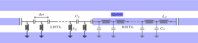
Figure 1: (color online). Discrete LHTL coupled to a continuous RHTL . The regular right-handed part of the transmission line is on the right, connected to a left-handed line shown on the left. The terminating capacitors allow to externally access the modes. The qubit couples to the right-handed component. In the supplementary material it is shown that stray capacitance to ground in the left handed line does not change the physics. Additional stray inductances and capacitances can be taken into account as shown by Eleftheriades, et al. Eleftheriades et al. (2002). The light blue areas indicate strip-lines and ground planes.

The System: In one-dimension, left-handedness is defined as the wave vector $\mathbf{k}_{l}$ and the Poynting vector having opposite orientation; the phase and group-velocity are opposite corresponding to a falling dispersion relation $\partial\omega(k)/\partial k<0$. This can be achieved Eleftheriades et al. (2002) by a discrete array of series capacitors and parallel inductors to ground, see Fig. 1. A low loss left-handed transmission line (LHTL) can be realized with superconductors Salehi et al. (2005); Jung et al. . This is the dual (inductors and capacitors interchanged) of the usual Pozar (2005) discrete representation of the right-handed transmission line (RHTL). In practice, the LHTL remains a metamaterial composed of discrete elements, whereas the RHTL is a metal strip represented as the continuum limit of a ladder network Pozar (2005). We can understand the physics of this line as follows: For any ladder network with discrete time-translation symmetry, the eigenmodes are (propagating or decaying) plane waves with a dispersion relation derived from the solutions of Pozar (2005)

$$\sin\left(\frac{k\Delta x}{2}\right)=\pm\frac{1}{2}i\sqrt{\frac{Z_{s}}{Z_{p}}}$$ (1)

For a RHTL, substituting impedances of the series elements $Z_{s}=i\omega L_{r}$ and parallel elements $Z_{p}=(i\omega C_{r})^{-1}$ gives the usual dispersion

$$\omega_{r}\left(k_{r}\right)=~{}\frac{2}{\sqrt{C_{r}L_{r}}}\sin\left(\frac{k_{r}\Delta x}{2}\right)\xrightarrow[\text{continuum}]{}\frac{k_{r}}{\sqrt{c_{r}l_{r}}}$$ (2)

For the LHTL, we interchange the roles of inductors and capacitors and obtain from equation (1) propagating modes (real-valued $k$ for real $\omega$) with the opposite dispersion relation

$$\omega_{l}\left(k_{l}\right)=~{}\frac{1}{2\sqrt{C_{l}L_{l}}\sin\left(\frac{k_{l}\Delta x}{2}\right)}$$ (3)

Here, $C_{l/r}$ and $L_{l/r}$ are capacitances and inductances as defined in Fig. 1 and $c_{r}$ and $l_{r}$ are the capacitance and inductance per unit length in the RHTL. $\Delta x$ is the size of a unit cell. More details are in the supplementary material.

Unusual physics arises when right- and left-handed media are interfaced Veselago (1968). We realize this with a coupled transmission line (CTL) shown in Fig. 1, a discrete LHTL coupled to a RHTL to be taken into the continuum limit. A key unusual feature of the LHTL, as compared to a regular RHTL, is the divergence of the density of modes (DoM) at a low-frequency bound $\omega_{\text{IR}}=1/2\sqrt{C_{l}L_{l}}$, seen in Fig. 2(a), implying the existence of a quasi-continuous band even in a cavity. In the LHTL, low frequencies correspond to short wavelengths due to the falling dispersion relation $\omega(k)$. Thus, by only a small change in frequency, a new orthogonal mode can be found that is different by one node in the left-handed component. As the wavelength approaches the lattice constant, the dispersion relation in equation (3) becomes flat due to Bragg reflection Ashcroft and Mermin (1976) — the DoM develops a van-Hove-type singularity setting the aforementioned divergence at $\omega_{\rm IR}$. Due to the hybrid nature of this new CTL, the closely spaced frequencies at this lower band-edge have nearly-identical spatial structures in the RHTL. The fast oscillation in the LHTL ensure orthogonality between modes. Figure 2(b) shows three consecutive low frequency modes obtained from the full solution. Close to $\omega_{\text{IR}}$ the RHTL provides a mere constant contribution thus the DoM is dominated by the divergence due to the LHTL and vice versa. In consequence, the DoM can be approximated by the sum of the densities in the uncoupled lines

$$\mathcal{D}\left(\omega\right)=\frac{4N_{l}\sqrt{C_{l}L_{l}}}{\pi}\tan\phi_{L}\sin\phi_{L},\quad\phi_{L}=\frac{k_{l}(\omega)\Delta x}{2}.$$

$N_{l}$ is the number of cells in the LHTL. The agreement between this prediction and the numerically obtained modes of the full model is excellent up to small oscillations, see Figure 2. To engineer the DOM, one can control $\omega_{\rm IR}$ by the mesh size and independently $N_{l}$ by the length of the LHTL.

To provide good coupling between both components one would like to have an impedance $Z_{0}$ (typically $50~{}\Omega$) requiring $C_{l}=(2\omega_{\text{IR}}Z_{0})^{-1}$ and $L_{l}=Z_{0}/2\omega_{\text{IR}}$. Furthermore for coupling to qubits $\omega_{\text{IR}}$ should be chosen to lie around qubit frequencies (e.g. $4$ GHz). The capacitances could be realized with interdigitated as well as with overlap capacitors and the parallel inductors could be realized with Josephson Junctions in the linear regime since they provide sufficient inductance in a small footprint. Furthermore it is shown in the supplementary material that disorder in these parameters has little effect.

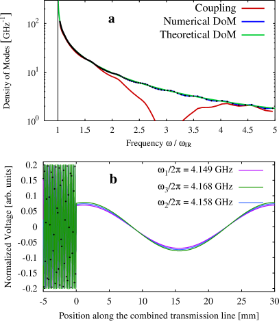
Figure 2: (color online). (a) Example of density of modes, showing a lower band-edge at $\omega_{\rm IR}$. Dots indicate actual modes, the green curve the approximate formula which is in excellent agreement. The red curve shows the coupling strength between a $0.5$ mm long flux qubit placed at a current anti-node of the transmission line, as in Fig. 1. Designing the qubit to couple to the $4.579~{}\mathrm{GHz}$ mode with strength $460~{}\mathrm{MHz}$, results in ultrastrong-coupling to 50 modes within a $\pm 460~{}\mathrm{MHz}$ range. (b) Example of the first three consecutive normal modes, the voltage profiles in the RHTL are almost identical. The LHTL has 200 unit cells measuring $100~{}\mathrm{\mu m}$ each. In the LHTL the voltages at the discrete unit cells, for the first mode only, are shown by the black dots; the continuous lines serve as a guide to the eye to see the mode structure. Requiring a $50~{}\Omega$ impedance and an IR cutoff at $\omega_{\text{IR}}/2\pi=4$ GHz sets $C_{l}=398~{}\mathrm{fF}$ and $L_{l}=995~{}\mathrm{pH}$. The parameters for the RHTL were chosen so that it supports a full wavelength at $\omega_{\text{IR}}$. This sets the values for its total inductance and capacitance. Therefore a $3~{}\mathrm{cm}$ long RHTL requires a capacitance and inductance per unit length of $c_{r}=1667~{}\mathrm{fF/\mu m}$ and $l_{r}=4167~{}\mathrm{pH/\mu m}$.

The quantum behavior of the CTL is obtained through canonical quantization of the circuit in Fig. 1. This leads to a system of uncoupled quantum harmonic oscillators, each described by operators $\hat{a}^{\dagger}_{n}$,$\hat{a}_{n}^{\phantom{\dagger}}$ acting on modes with frequencies $\omega_{n}$. A qubit described in its energy eigenbasis by Pauli matrices $\hat{\sigma}_{x/z}$ placed close to the CTL will couple to mode $n$ with strength $g_{n}$

$$\hat{H}/\hbar=\frac{\Delta_{0}}{2}\hat{\sigma}_{z}+\sum_{n}g_{n}\hat{\sigma}_{x}\left(\hat{a}_{n}^{\phantom{\dagger}}+\hat{a}_{n}^{\dagger}\right)+\sum_{n}\omega_{n}\hat{a}^{\dagger}_{n}\hat{a}_{n}^{\phantom{\dagger}}\,.$$ (4)

If the qubit is coupled to the RHTL, $g_{n}\simeq g_{n+1}$ for low frequency modes since they have similar spatial profiles in the RHTL. For a flux qubit Mooij et al. (1999); Clarke and Wilhelm (2008), the mode dependent part of the coupling strength is given by $\mathcal{D}(\omega_{n})\langle I_{n}(x)\rangle/\mathrm{max}_{n}\{\langle I_{n}(x)\rangle\}$. The current $I_{n}$ is averaged over the spatial extent of the qubit. Figure 2 shows that the qubit can be coupled to a wide range of modes. For frequencies sufficiently above $\omega_{IR}$ the wavelength in the RHTL also starts to change away from the antinode towards a node, creating a deep minimum in coupling strength. This mode structure allows the qubit to simultaneously couple to multiple modes when $N>1$ modes fall within a frequency interval of $2g_{n}$. We refer to this regime as multi-mode strong-coupling. It can be reached with other superconducting qubits, notably transmons Koch et al. (2007), which should be placed at a charge antinode. Flux qubits on the other hand allow us to reach multi-mode ultrastrong coupling Bourassa et al. (2009); Forn-Diaz et al. (2010) — $g_{n}/\omega_{n}>0.1$. This regime offers many new possibilities for circuit QED.

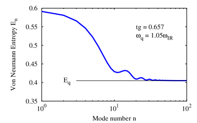
Figure 3: (color online). Von Neumann entropy as function of the traced out mode $n$. Here the qubit is put in the bath at a frequency $\omega_{q}>\omega_{\text{IR}}$ and the system left to evolve for a dimensionless time $tg$. The Von Neumann entropy is computed for the system after having traced out the qubit and mode $n$. We then vary $n$ to see how much the entropy increases from $E_{q}$, the entropy when only the qubit is traced out. $E_{q}>0$ indicates that their is at least bi-partite entanglement. When additionally tracing out mode $n$ the entropy $E_{n}$ increase above $E_{q}$ and this for all modes. The latter indicates complex multi-partite entanglement.

Applications: The multimode Rabi Hamiltonian, equation (4), allows us to prepare multimode entangled states. Within the rotating wave approximation it conserves the number of excitations. Exciting the qubit and placing its $0\leftrightarrow 1$ resonance frequency slightly above $\omega_{\rm IR}$ allows the qubit excitation to distribute itself over many modes, i.e., produce arbitrary superpositions of the form $c_{0}|1;0\rangle+\sum_{n}c_{n}|0;n\rangle$. $|0;n\rangle$ indicates the qubit in the ground state, a single photon in mode $n$ and none in the other modes. For $|1;0\rangle$ only the qubit is excited. These states are in general entangled as seen from their Von Neumann entropy Gühne and Toth (2009). Figure 3 shows the entropy, indicating multimode entanglement, of a single excitation, starting in $|1;0\rangle$, that spread out over all modes for a time $t$.

The Spin-Boson model Leggett et al. (1987) is a fundamental model of quantum dissipation which allows to understand the transition between coherent and incoherent behaviour as well as a quantum phase transition suppressing quantum tunneling. It is described by the Hamiltonian in equation (4) in the limit where the modes form a continuum. The dense modes at the low-frequency end provide a generic and realizable quantum simulator for this model. Our unusual density of modes provides a novel regime of sub-subhomic models with a low-frequency cutoff, i.e., a spectral density of the form

$$J(\omega)=\sum_{n}g_{n}^{2}\delta(\omega-\omega_{n})\simeq\frac{N_{l}}{\pi\sqrt{2\omega_{\text{IR}}}}\frac{\Theta(\omega-\omega_{\text{IR}})}{\sqrt{\omega-\omega_{\text{IR}}}}.$$

The ground and lowest excited states are well approximated by a multimode Schrödinger cat state of the qubit dressed by coherent photonic states Leggett et al. (1987)

$$|\pm\rangle=\frac{1}{\sqrt{2}}\left(|L\rangle\bigotimes_{n}|\lambda_{n}\rangle\pm|R\rangle\bigotimes_{n}|-\lambda_{n}\rangle\right).$$ (5)

$|L,R\rangle$ are the eigenstates of $\hat{\sigma}_{x}$. The renormalized energy splitting is

$$\Delta_{\rm eff}=\left\langle+\left|\hat{H}\right|-\right\rangle=\Delta_{0}\exp\bigg{(}-2\sum_{n}\lambda_{n}^{2}\bigg{)}.$$ (6)

The multimode cat state in equation (5) involves, according to the principle of adiabatic renormalization, all fast modes , those with $\omega_{n}>\Delta_{\rm eff}$, as they can adiabatically follow the qubit. Slow modes remain unaffected. Thus $\lambda_{n}=\frac{g_{n}^{2}}{\omega_{n}^{2}}\Theta(\omega_{n}-\Delta_{\rm eff})$ which leads to a self-consistency relation for $\Delta_{\rm eff}$. The ratio $\Delta_{\rm eff}/\Delta_{0}$ measures the accumulated phase space distance of the dressing clouds, i.e. the total cat size Haroche and Raimond (2006), by taking the logarithm of equation (6). Thus, the low-energy states of the system are strongly renormalized as are their effective energies.

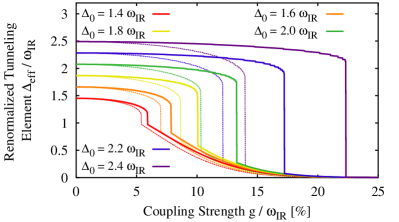
Figure 4: (color online). Plot of the renormalized tunnelling as function of the global coupling strength $g$. The individual mode coupling $g_{n}$ is the product of $g$ and the mode-dependent spatial contribution bounded by unity. The thin dashed lines correspond to the case when this effect is neglected i.e. $\langle I_{n}(x)\rangle/\max_{n}\{\langle I_{n}(x)\rangle\}=1$. This allows simultaneous tuning of the coupling to all modes. The discontinuous drop in $\Delta_{\text{eff}}$ distinguishes the regions of weakly and strongly renormalized energy splitting.

A true dissipative quantum phase transition Leggett et al. (1987); Weiss (1999) has $\Delta_{\rm eff}=0$ in the localised phase. This limit would be reached if the modes were infinitely close (hence arbitrarily close to $\omega_{\rm IR}$) as would result from an infinitely long LHTL or if $\omega_{\rm IR}\rightarrow 0$ as in the case of infinitely dense LHTL unit cells. Note that in the usual sub-Ohmic spin-boson model, the latter is assumed. We thus conclude that our system approaches a quantum phase transition in the infinite sample limit.

To corroborate the finite size-behaviour, we have studied the ground and first excited state of the qubit-CTL model using its actual modes in the adiabatic renormalization approach. We identify multiple regimes: for weak coupling or large $\Delta_{0}/\omega_{\rm IR}$, there is only weak dressing manifest by a small shift of $\Delta_{0}$. At stronger coupling, we observe the quasi-localized phase, with $\Delta_{\rm eff}\ll\Delta_{0}$. Remarkably, even at finite length, the two regimes are separated by a discontinuous transition as indicated by Figure 4. Figure 5 shows the corresponding finite-size phase diagram highlighting the need for ultrastrong coupling. We see that by tuning the bare qubit frequency slightly above the cutoff, $\Delta_{0}>\omega_{\rm IR}$ Paauw et al. (2009) we can tune the system through the phase transition in situ, or by employing a tunable coupler. The phase transition is manifest by a discontinuous drop in the energy splitting (as measured through spectroscopy) of the qubit that is inconsistent with the tuning of the circuit alone, see FIg. 4. Engineering the transmission line to have dense enough modes and an appropriate $\omega_{IR}$ can be accomplished using equation (Multimode circuit QED with hybrid metamaterial transmission lines) and $\omega_{IR}=1/2\sqrt{C_{l}L_{l}}$.

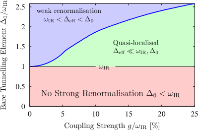
Figure 5: (color online). Finite-size phase diagram of the qubit-CTL system. The density of states for the case at hand is the same is in Fig. 2 with the dip in coupling taken into account.

On the level of partition functions, this model is equivalent to a one-dimensional Ising chain Cardy (1981); Weiss (1999). This is discussed in more detail in the supplementary material. In the present case, this would be an Ising chain with an interaction that decays as $\propto|i-j|^{-1/2}$, where $i$ and $j$ are site indices, up to a range $r\propto\omega_{\rm IR}^{-1}$, after which it decays exponentially. Thus, when cooled from high-temperatures the system is well described by mean-field theory, which predicts a ferromagnetic phase transition, until the correlation length reaches $r$. At that point, the system follows short-range physics and remains paramagnetic between magnetized blocks of size $r$ — in analogy to the tunnel coupling in the spin-boson model falling deeply, but not to zero.

In conclusion, we have proposed an engineered hybrid transmission line that allows to reach a new multimode strong coupling regime of circuit QED by combining a regular line with a metamaterial. This will open the way for novel applications in microwave photonics and strongly correlated photon states, out of which we have outlined the generation of multimode entanglement, multimode Schrödinger cat states and quantum phase transitions.

We acknowledge useful discussions with Heiko Rieger and Britton Plourde. We thank Emily Pritchett for her careful reading of the manuscript. This work was funded in parts by DARPA through the QuEST program and by the European Union through ScaleQIT.

References

- Haroche and Raimond (2006) S. Haroche and J.-M. Raimond, Exploring the Quantum: Atoms, Cavities, and Photons (Oxford University Press, Oxford, 2006).
- Blais et al. (2004) A. Blais, R.-S. Huang, A. Wallraff, S. M. Girvin, and R. J. Schoelkopf, Phys. Rev. A 69, 062320 (2004).
- Schoelkopf and Girvin (2008) R. Schoelkopf and S. Girvin, Nature 451, 664 (2008).
- You and Nori (2011) J. You and F. Nori, Nature 474, 589 (2011).
- Bourassa et al. (2009) J. Bourassa, J. M. Gambetta, A. A. Abdumalikov, O. Astafiev, Y. Nakamura, and A. Blais, Phys. Rev. A 80, 032109 (2009).
- Forn-Diaz et al. (2010) P. Forn-Diaz, J. Lisenfeld, D. Marcos, J. J. Garcia-Ripoll, E. Solano, C. J. P. M. Harmans, and J. E. Mooij, Phys. Rev. Lett. 105, 237001 (2010).
- Niemczyk et al. (2010) T. Niemczyk, F. Deppe, H. Huebl, E. P. Menzel, F. Hocke, M. J. Schwarz, J. J. Garcia-Ripoll, D. Zueco, T. Hümmer, E. Solano, et al., Nat. Phys. 6, 772 (2010).
- Filipp et al. (2011) S. Filipp, M. Göppl, J. M. Fink, M. Baur, R. Bianchetti, L. Steffen, and A. Wallraff, Phys. Rev. A 83, 063827 (2011).
- Mariantoni et al. (2008) M. Mariantoni, F. Deppe, A. Marx, R. Gross, F. K. Wilhelm, and E. Solano, Phys. Rev. B 78, 104508 (2008).
- Merkel and Wilhelm (2010) S. T. Merkel and F. K. Wilhelm, New J. Phys. 12, 093036 (2010).
- Wang et al. (2011) H. Wang, M. Mariantoni, R. C. Bialczak, M. Lenander, E. Lucero, M. Neeley, A. D. O’Connell, D. Sank, M. Weides, J. Wenner, et al., Phys. Rev. Lett. 106, 060401 (2011).
- Mariantoni et al. (2011) M. Mariantoni, H. Wang, R. C. Bialczak, M. Lenander, E. Lucero, M. Neeley, A. D. O’Connell, D. Sank, M. Weides, J. Wenner, et al., Nat. Phys. 7, 287 (2011).
- Nunnenkamp et al. (2011) A. Nunnenkamp, J. Koch, and S. M. Girvin, New J. Phys. 13, 095008 (2011).
- Hartmann et al. (2006) M. Hartmann, F. Brandao, and M. Plenio, Nat. Phys. 2, 849 (2006).
- Underwood et al. (2012) D. L. Underwood, W. E. Shanks, J. Koch, and A. A. Houck, Phys. Rev. A 86, 023837 (2012).
- Veselago (1968) V. Veselago, Sov. Phys. Usp. 10, 517 (1968).
- Pendry (2000) J. B. Pendry, Phys. Rev. Lett. 85, 3966 (2000).
- Eleftheriades et al. (2002) G. Eleftheriades, A. Izer, and P. Kremer, IEEE Trans. Microwave Theory and Techniques 50, 2702 (2002).
- Salehi et al. (2005) H. Salehi, A. H. Majedi, and R. R. Mansour, IEEE Trans. Appl. Superconductivity 15, 996 (2005).
- (20) P. Jung, S. Butz, S. V. Shitov, and A. V. Ustinov, arXiv.1301.0440v1.
- Pozar (2005) D. Pozar, Microwave Engineering (Wiley, New York, 2005), 3rd ed.
- Ashcroft and Mermin (1976) N. Ashcroft and N. Mermin, Solid state physics (Holt-Saunders, 1976).
- Mooij et al. (1999) J. E. Mooij, T. P. Orlando, L. Levitov, L. Tian, C. H. van der Wal, and S. Lloyd, Science 285, 1036 (1999).
- Clarke and Wilhelm (2008) J. Clarke and F. K. Wilhelm, Nature 453, 1031 (2008).
- Koch et al. (2007) J. Koch, T. M. Yu, J. Gambetta, A. A. Houck, D. I. Schuster, J. Majer, A. Blais, M. H. Devoret, S. M. Girvin, and R. J. Schoelkopf, Phys. Rev. A 76, 042319 (2007).
- Gühne and Toth (2009) O. Gühne and G. Toth, Physics Reports 474, 1 (2009).
- Leggett et al. (1987) A. Leggett, S. Chakravarty, A. Dorsey, M. Fisher, A. Garg, and W. Zwerger, Rev. Mod. Phys. 59, 1 (1987).
- Weiss (1999) U. Weiss, Quantum Dissipative Systems, no. 10 in Series in modern condensed matter physics (World Scientific, Singapore, 1999), 2nd ed.
- Paauw et al. (2009) F. G. Paauw, A. Fedorov, C. J. P. M. Harmans, and J. E. Mooij, Phys. Rev. Lett. 102, 090501 (2009).
- Cardy (1981) J. Cardy, J. Phys. A: Math. Gen. 14, 1407 (1981).