Exotic spin orders driven by orbital fluctuations in the Kugel-Khomskii model

Abstract

We study zero temperature phase diagram of the three-dimensional Kugel-Khomskii model on a cubic lattice using the cluster mean field theory and different perturbative expansions in the orbital sector. The phase diagram is rich, goes beyond the single-site mean field theory due to spin-orbital entanglement. In addition to the antiferromagnetic (AF) and ferromagnetic (FM) phases, one finds also a plaquette valence-bond phase with singlets ordered either on horizontal or vertical bonds. More importantly, for increasing Hund’s exchange we identify three phases with exotic magnetic order stabilized by orbital fluctuations in between the AF and FM order: (i) an AF phase with two mutually orthogonal antiferromagnets on two sublattices in each $ab$ plane and AF order along the $c$ axis (ortho-$G$-type phase), (ii) a canted-$A$-type AF phase with a non-trivial canting angle between nearest neighbor FM layers along the $c$ axis, and (iii) a striped-AF phase with anisotropic AF order in the $ab$ planes. We elucidate the mechanism responsible for each of the above phases by deriving effective spin models which involve second and third neighbor Heisenberg interactions as well as four-site spin interactions going beyond Heisenberg physics, and explain how the entangled nearest neighbor spin-orbital superexchange generates spin interactions between more distant spins.
    Published in Physical Review B 87, 064407 (2013).

I Introduction

Recent interest and progress in the theory of spin-orbital superexchange models was triggered by the observation that orbital degeneracy drastically increases quantum fluctuations (QF) which may suppress long-range order in the regime of strong competition between different types of ordered states near the quantum critical point.Feiner et al. (1997) The simplest and archetypical three-dimensional (3D) model for the spin-orbital physics is the Kugel–Khomskii (KK) model introduced for KCuF₃ by Kugel and Khomskii long ago.Kugel and Khomskii (1973); *Kug82 KCuF₃ is a strongly correlated system with a single hole within degenerate $e_{g}$ orbitals at each Cu²⁺ ion. Kugel and Khomskii showed that interactions between strongly correlated electrons could then stabilize orbital order by a purely electronic mechanism, the superexchange. A similar situation occurs in a number of compounds with active orbital degrees of freedom, where strong on-site Coulomb interactions localize electrons (or holes) and give rise to spin-orbital superexchange. Tokura and Nagaosa (2000); van den Brink et al. (2011); Khaliullin (2005); Oleś et al. (2005); Oleś (2012)

The orbital superexchange may stabilize the orbital order by itself, but in $e_{g}$ systems it is usually helped by the Jahn-Teller distortions of the lattice which generate effective intersite orbital interactions. Zaanen and Oleś (1993); Feiner and Oleś (1999); van den Brink et al. (1999) For instance, in LaMnO₃ the terms that originate from the superexchange and the Jahn-Teller distortions are of equal importance and both are necessary to explain the observed high temperature $T_{\rm OO}\simeq 780K$ of the structural transition.Feiner and Oleś (1999) Also in KCuF₃ the lattice distortions play an important role Paolasini et al. (2002); *Cac02; *Bin04; Deisenhofer et al. (2008); Leonov et al. (2010) and are responsible for its strongly anisotropic magnetic and optical properties. The latest theoretical and experimental results for this compound show that other types of interactions, like Goodenough processes in the superexchange,Oleś et al. (2005) direct orbital exchange driven by a combination of electron–electron interactions and ligand distortions, Lee et al. (2012) or dynamical Dzyaloshinsky-Moriya interaction,Eremin et al. (2008) are necessary to explain structural phase transition in KCuF₃ at $T_{\rm OO}\simeq 800K$ and peculiarities in spin dynamics.Yamada and Kato (1994) The compound itself is believed to be the best realization of the one-dimensional (1D) antiferromagnetic (AF) Heisenberg model above the Néel temperature $T_{N}=39K$,Lake et al. (2005) and spinon excitations were indeed observed in neutron scattering.Tennant et al. (1993)

While the coexisting $A$-type AF ($A$-AF) order and the orbital order are well established in KCuF₃ below the Néel temperature $T_{N}\simeq 39$ K,Lee et al. (2012) and this phase is reproduced by the spin-orbital $d^{9}$ superexchange model in the mean field (MF) approximation,Oleś et al. (2000) the phase diagram of this model is still unknown beyond the MF approach because of strongly coupled spin and orbital degrees of freedomFeiner et al. (1997, 1998) which poses an outstanding question in the theory: Which types of coexisting spin and orbital order (or disorder) are possible when its microscopic parameters (splitting of the $e_{g}$ orbitals $E_{z}$ and Hund’s exchange $J_{H}$) are varied? So far, it was suggested that the long-range AF order is destroyed by spin-orbital QF,Feiner et al. (1997, 1998) but another possibility that the ordered state might be stabilized by the order-out-of-disorder mechanism was also pointed out in the regime of ferro-orbital (FO) order of $3z^{2}-r^{2}$ orbitals.Khaliullin and Oudovenko (1997) An alternative to magnetic order are spin-disordered phases with pronounced valence-bond spin-orbital correlations, as suggested by simple variational wave functions.Feiner et al. (1997)

The purpose of this paper is to investigate the phase diagram of the 3D KK model, in the presence of spin-orbital QF. This subject is of interest in the broad context of frustration in magnetic systems,Normand (2009); Balents (2010) which appears to be intrinsic for the orbital superexchange.Feiner et al. (1997); Cincio et al. (2010) To establish reliable results concerning short-range order in the crossover regime between phases with long-range AF or ferromagnetic (FM) order, we developed a cluster MF approach which goes beyond the single-site MF in the spin-orbital system Silva et al. (2003) and is based on an exact diagonalization of a cluster coupled to its neighbors by the MF terms. The cluster is chosen to be sufficient for investigating both AF phases with four sublattices and valence-bond states, with spin singlets either along the $c$ axis or within the $ab$ planes. This theoretical approach is motivated by possible spin-orbital entanglementOleś et al. (2006); Oleś (2012) which is particularly pronounced in the 1D SU(4) [or SU(2)$\otimes$SU(2)] spin-orbital modelFrischmuth et al. (1999); *Ole07; *You12 and occurs also on the frustrated triangular lattice,Normand and Oleś (2008); *Nor11; *Cha11; *Tro12 and in the models for perovskites when spin correlations are AF on the bonds Oleś (2012) — then the Goodenough-Kanamori rulesGoodenough (1963); *Kan59 are violated in some cases. In the perovskite vanadates such entangled states play an important role at finite temperature: in their optical properties,Khaliullin et al. (2004) in the phase diagram,Horsch et al. (2008) and in the dimerization of FM interactions along the $c$ axis in the $C$-AF phase of YVO₃,Ulrich et al. (2003); *Hor03 understood within the 1D spin-orbital model.Sirker et al. (2008); *Sir03; *Her11 Previous studies employing the cluster MF approach have shown that phases with entangled spin-orbital degrees of freedom occur in the KK bilayer,Brzezicki and Oleś (2011); *cam11 while a noncollinear spin order emerges from entangled spin-orbital fluctuations in the two-dimensional (2D) KK monolayer.Brzezicki et al. (2012) Below we investigate whether spin-orbital entangled states could also play a role in the present 3D KK model.

The paper is organized as follows. In Sec. II.1 we briefly introduce the spin-orbital superexchange in the KK model. As the first approximation, in Sec. II.2 we present the phase diagram of the model obtained in the single-site MF approximation — this approach ignores any possible spin-orbital entanglement. To include the effects of spin-orbital QF we introduce the cluster MF method for the 3D system in Sec. III.1, with two different topologies of the cluster, and present the phase diagram modified by spin-orbital entanglement in Sec. III.1. It contains three phases with exotic magnetic order: the ortho-$G$-AF phase similar to that found recently for the monolayer,Brzezicki et al. (2012) the canted-$A$-AF phase, and the striped-AF phase. Next we present the behavior of the order parameters, spin angles, total magnetization, correlations and spin-orbital covariances for two paths in the phase diagram which include certain exotic phases: (i) from the $A$-AF through canted-$A$-AF to FM phase in Sec. III.3, and (ii) from the striped-AF to $G$-AF phase in Sec. III.4. As we show in Sec. III.5, rather weak orbital fluctuations are found in several phases and the orbital moments are reduced by them. Then we explain and highlight the origin of the exotic magnetic phases by deriving effective spin Hamiltonians within perturbative expansion in the orbital sector. Spin models for the ortho-G-AF phase, canted-$A$-AF phase, and striped-AF phase are derived in Secs. IV.1, IV.2, and IV.4, respectively. In Sec. IV.3, using a similar perturbative expansion, we explain the absence of the $C$-AF phase in the phase diagram of the KK model obtained within the cluster MF approximation. Summary and conclusions are given in Sec. V, while certain additional details of the performed perturbative analysis are presented in Appendices A-C.

II The Kugel–Khomskii model

II.1 Frustrated spin-orbital superexchange

For realistic parameters the late transition metal oxides or fluorides are strongly correlated and electrons localize in the $3d$ orbitals, Oleś et al. (1987); *Grz91; Grant and McMahan (1992) leading in cuprates to Cu²⁺ ions with spin $S=1/2$ in $d^{9}$ configuration and $e_{g}$ orbitals occupied by one hole:

$$|x\rangle\equiv(x^{2}-y^{2})/\sqrt{2},\hskip 14.22636pt|z\rangle\equiv(3z^{2}-r^{2})/\sqrt{6}\,.$$ (1)

The examples of such systems are: KCuF₃ with 3D cubic lattice, K₃Cu₂F₇ representing bilayer compounds, and K₂CuF₄ and La₂CuO₄ with 2D square lattice. We also use below the short-hand notation for the orbital basis, $\{x,z\}$. Here $t_{2g}$ orbitals are split in the octahedral field and do not couple to $e_{g}$’s by hopping through fluorine, so they can be neglected. In what follows we investigate the 3D spin-orbital superexchange model obtained by considering charge excitations between transition metal ions,Oleś et al. (2000) $d_{i}^{9}d_{j}^{9}\rightleftharpoons d_{i}^{8}d_{j}^{10}$ in the regime of large $U$, and neglect the coupling to lattice distortions arising due to the Jahn-Teller lattice distortions.

One finds the Heisenberg Hamiltonian for $S=\frac{1}{2}$ spins coupled to the orbital problem,

$${\cal H}=-\frac{1}{2}J\sum_{\gamma=a,b,c}\sum_{\langle ij\rangle||\gamma}H_{ij}^{\gamma}-E_{z}\sum_{i}\tau_{i}^{c},$$ (2)

where bond-interaction terms $H_{ij}^{\gamma}$ are defined as follows,

$$H_{ij}^{\gamma} = \left(r_{1}\,\Pi_{t}^{(ij)}+r_{2}\,\Pi_{s}^{(ij)}\right)\left(\frac{1}{4}-\tau_{i}^{\gamma}\tau_{j}^{\gamma}\right)$$ (3)

$$+ \left(r_{2}+r_{4}\right)\Pi_{s}^{(ij)}\left(\frac{1}{2}-\tau_{i}^{\gamma}\right)\left(\frac{1}{2}-\tau_{j}^{\gamma}\right).$$

Here $\gamma=a,b,c$ labels the direction of a bond $\langle ij\rangle$ in the 3D system. The energy scale is given by the superexchange constant,

$$J=\frac{4t^{2}}{U},$$ (4)

where the hopping $t$ is the effective intersite $(dd\sigma)$ hopping element for an $e_{g}$ hole between $z$ orbitals along the $c$ axis, Zaanen and Oleś (1993) and the other $e_{g}$ hopping elements obey the cubic symmetry.Feiner and Oleś (2005) The orbital operators at site $i$ are $\vec{\tau}_{i}=\{\tau_{i}^{a},\tau_{i}^{b},\tau_{i}^{c}\}$. These operators represent $e_{g}$ orbital degrees of freedom, have cubic symmetry in the 3D lattice and are expressed in terms of Pauli matrices $\{\sigma_{i}^{x},\sigma_{i}^{y},\sigma_{i}^{z}\}$ in the following way:

$$\tau_{i}^{a(b)}\equiv\frac{1}{4}(-\sigma_{i}^{z}\pm\sqrt{3}\sigma_{i}^{x}),\hskip 14.22636pt\tau_{i}^{c}\equiv\frac{1}{2}\sigma_{i}^{z}.$$ (5)

The matrices $\{\sigma_{i}^{\gamma}\}$ act in the orbital space (and have nothing to do with the physical spin ${\bf S}_{i}$ present in this problem). Note that $\{\tau_{i}^{\gamma}\}$ operators are not independent from one another because they satisfy the local constraint, $\sum_{\gamma}\tau_{i}^{\gamma}\equiv 0$. The operators $\Pi_{ij}^{s}$ and $\Pi_{ij}^{t}$ stand for projections of spin states on the bond $\langle ij\rangle$ on a singlet ($\Pi_{ij}^{s}$) and triplet ($\Pi_{ij}^{t}$) configuration, respectively,

$$\Pi_{s}^{(ij)}=\left(\frac{1}{4}-{\bf S}_{i}\cdot{\bf S}_{j}\right),\hskip 14.22636pt\Pi_{t}^{(ij)}=\left(\frac{3}{4}+{\bf S}_{i}\cdot{\bf S}_{j}\right),$$ (6)

for spins $S=\frac{1}{2}$ at both sites $i$ and $j$ of the bond $\langle ij\rangle$. Spin interactions obey the SU(2) symmetry. More details on the derivation of Eq. (3) may be found in Ref. Oleś et al., 2000.

The model Eq. (2) depends thus on two parameters: Oleś et al. (2000) (i) Hund’s exchange coupling $\eta$, and (ii) the crystal-field splitting of $e_{g}$ orbitals $E_{z}/J$. The first of them is given by the ratio of Hund’s exchange $J_{H}$ and intraorbital Coulomb element $U$ defined in a standard way as in the degenerate Hubbard model,Oleś (1983)

$$\eta\equiv\frac{J_{H}}{U},$$ (7)

and determines the values of the coefficients in Eq. (3):

$$r_{1}=\frac{1}{1-3\eta},\hskip 14.22636ptr_{2}=\frac{1}{1-\eta},\hskip 14.22636ptr_{4}=\frac{1}{1+\eta}.$$ (8)

The typical energies for the Coulomb $U$ and Hund’s exchange $J_{H}$ can be deduced from the atomic spectra or from density functional theory with constrained electron densities. Earlier studies performed within the local density approximation (LDA) gave rather large values of the interaction parameters for Cu²⁺ ions: Grant and McMahan (1992) $U=8.96$ eV and $J_{H}=1.19$ eV. More recent studies used the Coulomb interactions treated within the LDA+$U$ scheme and gave somewhat reduced values:Liechtenstein et al. (1995) $U=7.5$ eV and $J_{H}=0.9$ eV. However, both parameter sets give a rather similar value of Hund’s exchange parameter $\eta$, being within the expected range $0.10<\eta<0.15$ for strongly correlated late transition metal oxides. Oleś et al. (2005) Note that the physically acceptable range is much broader, i.e., $0<\eta<1/3$. The upper limit follows from the condition $(U-3J_{H})>0$ for the high-spin excitation energy.

The last term of the $H_{e_{g}}$ Hamiltonian (2) lifts the degeneracy of the two $e_{g}$ orbitals,

$$H_{z}=-\frac{1}{2}E_{z}\sum_{i}(n_{ix}-n_{iz})\equiv-E_{z}\sum_{i}\tau_{i}^{c}\,,$$ (9)

where $\{n_{ix\sigma},n_{iz\sigma}\}$ are hole number operators in $\{x,z\}$ orbitals (1) at site $i$. It favors hole occupancy of $x$ ($z$) orbitals when $E_{z}>0$ ($E_{z}<0$) and can be associated with a uniaxial pressure along the $c$ axis or a crystal-field splitting induced by a static Jahn-Teller effect.

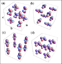
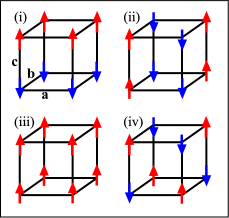
Figure 1: (Color online) Left panel: schematic view of four representative orbital configurations on a representative cube of the 3D lattice: (a) AO order with $\langle\tau_{i}^{a(b)}\rangle=1/2$ changing from site to site and $\langle\tau_{i}^{c}\rangle=-1/4$, obtained for $E_{z}<0$, (b) AO order with $\langle\tau_{i}^{a(b)}\rangle=-1/2$ changing from site to site and $\langle\tau_{i}^{c}\rangle=1/4$, obtained for $E_{z}>0$, (c) FO order with occupied $z$ orbitals and $\langle\tau_{i}^{c}\rangle=-1/2$ (cigar-shaped orbitals), and (d) FO order with occupied $x$ orbitals and $\langle\tau_{i}^{c}\rangle=1/2$ (clover-shaped orbitals). Right panel: schematic view of four representative spin configurations (arrows stand for up or down spins) shown on a cubic cluster: (i) $A$-AF configuration, (ii) $C$-AF configuration, (iii) FM configuration, and (iv) $G$-AF configuration.

In Figs. 1(a)-1(d) we present typical orbital configurations with FO order and alternating orbital (AO) order considered in the $e_{g}$ orbital models.van den Brink et al. (1999); Feiner and Oleś (2005) In the next sections we analyze their possible coexistence with spin order in the KK model Eq. (2). As we can see, the maximal (minimal) value of the orbital operators $\tau_{i}^{\gamma}$ is related with orbital taking shape of a clover (cigar) with symmetry axis pointing along the direction $\gamma$.

II.2 Phase diagram in single-site mean field

After averaging over spins, the Hamiltonian of Eq. (2), originally expressed in terms of bond operators, can be rewritten as an effective orbital Hamiltonian,

$${\cal H}_{{\rm MF}}\! = \frac{1}{2}J\sum_{i,\gamma}\left\{\tau_{i}^{\gamma}\tau_{i+\gamma}^{\gamma}(\chi^{\gamma}-\xi^{\gamma})+\tau_{i}^{\gamma}\xi^{\gamma}-\frac{1}{4}(\chi^{\gamma}+\xi^{\gamma})\right\}$$ (10)

$$- E_{z}\sum_{i}\tau_{i}^{c},$$

where $i$ runs over sites of the cubic lattice, and $i+\gamma$ is the nearest neighbor (NN) of site $i$ along the axis $\gamma=a,b,c$. The coefficients,

$$\chi^{\gamma}=r_{1}\Pi_{t}^{\gamma}+r_{2}\Pi_{s}^{\gamma},\hskip 14.22636pt\xi^{\gamma}=(r_{2}+r_{4})\Pi_{s}^{\gamma},$$ (11)

are parameters obtained by averaging of the spin projectors in Eq. (6) under assumption that the spin order depends only on the direction $\gamma$ and all the bonds $\langle i,i+\gamma\rangle$ along the axis $\gamma$ are equivalent:

$$\Pi_{s}^{\gamma}=\frac{1}{4}-\langle{\bf S}_{i}\cdot{\bf S}_{i+\gamma}\rangle,\hskip 14.22636pt\Pi_{t}^{\gamma}=\frac{3}{4}+\langle{\bf S}_{i}\cdot{\bf S}_{i+\gamma}\rangle.$$ (12)

In the single-site MF the spin QF are absent at zero temperature and the projectors can be replaced by their average values. This is sufficient to investigate the phases with either AF or FM long-range order.

Table 1: Mean values of triplet $\Pi_{t}^{\gamma}$ and singlet $\Pi_{s}^{\gamma}$ projection operators Eqs. (12) for a bond $\langle ij\rangle$ along the axis $\gamma=a,b,c$ in different phases with long-range magnetic order which occur in the MF phase diagram, see Figs. 1(i)-1(iv).

Phase	$\Pi_{t}^{a(b)}$	$\Pi_{t}^{c}$	$\Pi_{s}^{a(b)}$	$\Pi_{s}^{c}$
$G$-AF	1/2	1/2	1/2	1/2
$C$-AF	1/2	1	1/2	0
$A$-AF	1	1/2	0	1/2
FM	1	1	0	0

The values of the projection operators (12) depend on the assumed spin order. Here we consider four different spin configurations shown in Fig. 1: (i) $A$-AF phase — with FM order in the $ab$ planes and AF correlations along the $c$ axis [Fig. 1(i)], (ii) $C$-AF phase — with AF order in the $ab$ planes and FM correlations along the $c$ axis [Fig. 1(ii)], (iii) FM phase [Fig. 1(iii)], and (iv) $G$-AF phase Néel state [Fig. 1(iv)]. In the single-site MF approximation we use the classical average values of the spin projection operators in the above phases listed in Table 1. Apart from fully AF and FM phase we include also $A$-AF ($C$-AF) configurations with spin correlations being AF along the $c$ axis (in the $ab$ planes), and FM otherwise. Solutions of the self-consistency equations and ground state energies in different phases can be obtained analytically, as shown in Ref. Brzezicki and Oleś, 2011.

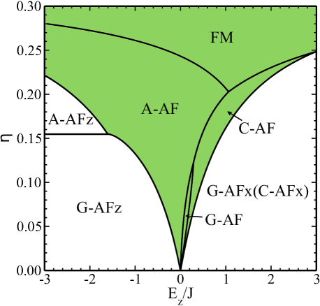
Figure 2: (Color online) Phase diagram of the 3D KK model obtained in the single-site MF approximation. Shaded dark gray (green) area indicates phases with AO order while the remaining magnetic phases are accompanied by FO order with fully polarized orbitals, either $x$ (for $E_{z}>0$) or $z$ (for $E_{z}<0$). In this approach the $G$-AF$x$ and $C$-AF$x$ phases with FO order are degenerate.

The phase diagram presented in Fig. 2 was obtained by purely energetic considerations — it shows the border lines between phases with the lowest energies in the $(E_{z},\eta)$ plane. Remarkably, this phase diagram is almost the same as the one obtained for the bilayer systemBrzezicki and Oleś (2011) — the same phases were found both in the 3D and in the bilayer KK model, and the major difference is the location of the multicritical point, being now at $(E_{z},\eta)=(0,0)$. This reflects the cubic symmetry in the model (2) at $E_{z}=0$, while this symmetry is broken by the crystal-field term in both planar models — indeed, for the KK bilayer the multicritical point is located at $(E_{z},\eta)=(-0.25J,0)$,Brzezicki and Oleś (2011) and it is moved further to $(E_{z},\eta)=(-0.5J,0)$ for the monolayer KK model. Brzezicki et al. (2012) At $\eta=0$ one finds only two AF phases: (i) $G$-AF$z$ for $E_{z}<0$ and (ii) $G$-AF$x$ for $E_{z}>0$, both with polarized orbital configuration (FO order) which involves either cigar-shaped $z$ orbitals in the $G$-AF$z$ phase, see Fig. 1(c), or clover-shaped $x$ orbitals in the $G$-AF$x$, see Fig. 1(d). Because of the planar orbital configuration in the $G$-AF$x$ phase one finds no interplane exchange coupling — thus the spin order along the $c$ axis is undetermined and this phase is degenerate with the $C$-AF one. This degeneracy is lifted in the cluster MF approach, see below.

For higher $\eta$ the number of phases increases abruptly by those with AO configurations (green areas), as shown in Figs. 1(a) and 1(b), coexisting with different possible spin orders: the $A$-AF, $C$-AF, $G$-AF and FM phases, respectively. Altogether, the phase diagram obtained here reproduces qualitatively the one obtained before for the simplified model using the lowest order expansion in $\eta$.Feiner et al. (1997) The $C$-AF phase occurs in a narrow range of parameters in between the $G$-AF and either $A$-AF or FM phase.

In contrast to the FO phases, the AO order in the shaded phases is never trivial in the sense that the orbitals are never fully polarized in any direction, which is a feature of the self-consistent MF solution (see Ref. Brzezicki and Oleś, 2011). The only new phase with FO configuration is the $A$-AF$z$ one appearing above $\eta=0.155$ for $E_{z}<0$. On the other hand, the FM spin order coexists solely with alternating orbitals. Finally, the new exotic magnetic phases reported in Sec. III (ortho-$G$-A, canted-$A$-AF, and striped-AF phase) cannot appear here as their stabilizing mechanism is absent in the single-site MF, so they are not included in Table 1.

III Cluster mean field approach

III.1 Clusters and order parameters

Following the ideas from Ref. Brzezicki and Oleś, 2011 and Brzezicki et al., 2012, to obtain more insight into the phase diagram of the 3D KK model and to include the QF and spin-orbital entanglement on the bonds, we divide the lattice into clusters, either plaquettes shown in Fig. 3(a), or chain clusters shown in Fig. 3(b). The most natural choice of the cluster would be a cube with eight sites as it was done in the bilayer caseBrzezicki and Oleś (2011) but, since we want to keep two components of the spin order parameter, we adopted here a simpler and less time-consuming approach using four-site clusters. The geometry of the selected clusters depends on the direction in which we expect a large energy gain due to QF. For example, if we want to study the transition between the $G$-AF and $A$-AF phases then the reasonable cluster topology is a square in the $ab$ plane, shown in Fig. 3(a), because the order along the $c$ axis does not change across the transition. On the other hand, if we are interested in a transition between the $A$-AF and FM phase where the order in the $ab$ planes remains constant, then a better choice is a chain along the $c$ axis — see Fig. 3(b).

The interactions along bonds corresponding to the solid lines in Fig. 4 are treated by exact diagonalization as they stand in the 3D KK model (2), while the bonds represented by dashed lines are decoupled in the MF approximation using the approximate identity for any bond operator:

$$O_{i}O_{j} \approx O_{i}\langle O_{j}\rangle-\frac{1}{2}\langle O_{i}\rangle\langle O_{j}\rangle$$ (13)

$$+ O_{j}\langle O_{i}\rangle-\frac{1}{2}\langle O_{i}\rangle\langle O_{j}\rangle\,.$$

To simulate infinite 3D lattice we need MF bonds in all three directions. Now we assume that site $i$ belongs to a chosen cluster and $j$ belongs to a neighboring one, and the bond is splitted into two halves — the first one is added to the Hamiltonian of the cluster $i$ and the other one to the cluster $j$. In this way the original KK Hamiltonian transforms into the sum of commuting cluster Hamiltonians interacting via MF terms.

The MFs follow from Eq. (13) applied to all the two-site operator products encountered in the Hamiltonian (2) and are defined as follows:

$$s_{i}^{\alpha}\equiv\left\langle S_{i}^{\alpha}\right\rangle,\hskip 14.22636ptt_{i}^{\gamma}\equiv\left\langle\tau_{i}^{\gamma}\right\rangle,\hskip 14.22636ptv_{i}^{\alpha,\gamma}\equiv\left\langle S_{i}^{\alpha}\tau_{i}^{\gamma}\right\rangle\,.$$ (14)

Here $\alpha=x,z$, $\gamma=a,b$ ($\gamma=c$) and $i=1,2,3,4$ for the cluster sites of a plaquette (chain) cluster, see Fig. 3. Note that the SU$(2)$ symmetry of the spin sector does not need to be broken in the $z$ spin direction ($\alpha=z$), but we also allow $\alpha=x$ to capture more exotic types of magnetic order suggested by the results reported recently for the 2D system.Brzezicki et al. (2012) However, we do not need to consider $\alpha=y$ because the KK Hamiltonian is real.

Figure 3: Schematic view of the clusters (solid lines) used in the cluster MF approach of Sec. III to the 3D KK model: (a) a plaquette in the $ab$ plane, and (b) a chain along the $c$ axis. Vertices $i=1,2,3,4$ and directions $\gamma=a,b,c$ are marked; dashed lines stand for the outgoing bonds where the spin-orbital interactions are replaced by the MF terms at neighboring sites, see Eq. (13).

To obtain the unbiased and the most general phase diagram, we do not assume anything about the order inside the cluster because the considered plaquette is small enough to keep the order parameters at all its sites as independent variables along the MF iteration process. Nevertheless, we still need to relate different clusters to one another to make the problem solvable. In the case of a square cluster we assume that the neighboring clusters in the $c$ direction can have either the same spin or inverted spin configuration (it gives either FM or AF bonds along $c$ axis). Furthermore, we assume that the neighbors in the $ab$ plane can have either the same orbital configuration that gives AO and FO orders in the $ab$ planes, or the orbital configuration is rotated by $\pi/2$ in the $ab$ plane — it gives the plaquette valence-bond (PVB) phase. Similarly, we assume that the chain clusters are copied without any change along the $c$ axis and the neighboring chains in the $ab$ planes have: (i) orbital configuration rotated by $\pi/2$, and (ii) spin configuration either inverted (it gives planar AF order) or unchanged (it gives planar FM order). All these assumptions are necessary to solve the self-consistent cluster MF problem and are motivated by the phase diagrams of the bilayer and the monolayer systems (see Refs. Brzezicki and Oleś, 2011 and Brzezicki et al., 2012).

The self–consistency equations still cannot be solved exactly because the effective cluster Hilbert space is of the size $d=2^{8}$ which is too large for analytical methods. The way out is to use Bethe–Peierls–Weiss method, i.e., to set certain initial values for the order parameters Eq. (14), $\{s_{i}^{\alpha},t_{i}^{\gamma},v_{i}^{\alpha,\gamma}\}$, and next to employ numerical diagonalization algorithm to the cluster Hamiltonian. We recalculate the order parameters, $\{s_{i}^{\alpha},t_{i}^{\gamma},v_{i}^{\alpha,\gamma}\}$, along the iteration process, and this procedure is repeated until the convergence conditions for energy and order parameters are satisfied.

III.2 Phase diagram

The phase diagram obtained in the cluster MF approach is shown in Fig. 4. One finds the phases with magnetic long-range order, obtained in the single-site MF and explained in Sec. II.2, in the broad (unshaded) part of the phase diagram: the $G$-AF, $A$-AF and FM phase. The shading in the center marks the spin disordered PVB phase with pairs of spin singlets alternating in the $ab$ planes and accompanied by $z$-like $3x^{2}-r^{2}/3y^{2}-r^{2}$ orbitals pointing along the singlet bonds.Feiner et al. (1997) Analogous valence-bond phases were also found in the bilayerBrzezicki and Oleś (2011) and monolayer Brzezicki et al. (2012) KK model. The darker (orange) shading indicates exotic magnetic orders which can be found when some AF spin interactions change into FM ones; they are: (i) ortho-$G$-AF phase already encountered in the 2D KK model and called there ortho-AF phase,Brzezicki et al. (2012) (ii) canted-$A$-AF phase, and (iii) striped-AF phase. These new phases arise from orbital fluctuations in the regimes of strongly frustrated spin-orbital superexchange, as explained below.

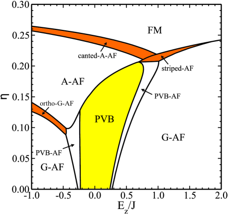
Figure 4: (Color online) Phase diagram of the 3D KK model in the cluster MF approximation. Plaquette valence-bond (PVB) phase with alternating spin singlets in the $ab$ planes, highlighted in light gray (yellow), occurs between the phases with magnetic long-range order, see Fig. 1. Phases with exotic magnetic order are shaded in dark gray (orange).

We begin with the ortho-$G$-AF phase, with the spin order consisting of two interpenetrating AF sublattices in the $ab$ planes, as shown in Fig. 5. This configuration repeats itself in the next $ab$ plane but all spins are inverted, meaning AF order along the $c$ axis. Note that this phase separates phases with antiferromagnetism ($G$-AF) and ferromagnetism ($A$-AF) within $ab$ planes, as found before in the 2D KK model.Brzezicki et al. (2012) The interactions along the $c$ axis are compatible with the in-plane magnetic order and even stabilize it as one finds here the ortho-$G$-AF phase at a given $\eta$ for a lower value of $E_{z}$ than that in the 2D phase. The ortho-$G$-AF phase with interplanar antiferromagnetism replaces here the resonating valence-bond (RVB) phase found before in the 3D KK model,Feiner et al. (1997) where it was proposed as an intermediate phase separating the $G$-AF and $A$-AF phases. We believe that the present result is more realistic (at zero temperature) than the RVB phase within 1D chains along the $c$ axis found before Feiner et al. (1997) — this latter phase would be easily modified by any in-plane magnetic order because the 1D Heisenberg antiferromagnet is critical and thus easily destabilized. In addition, orbital fluctuations remove locally AF spin coupling and thus block the resonance in the RVB phase. We argue below that the ortho-$G$-AF phase is well justified by the effective perturbative spin model derived for the 2D KK model in Ref. Brzezicki et al., 2012 and for the present 3D model in Sec. IV.1.

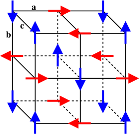
Figure 5: (Color online) Classical view of the ortho-$G$-AF spin order realized in the 3D KK model within $ab$ planes, and staggered along the $c$ axis. Vertical and horizontal arrows correspond to two interpenetrating AF states on the sublattices of next nearest neighbor sites. Up (down) arrows stand for $\left\langle S_{i}^{z}\right\rangle=\pm 1/2$, right (left) arrows stand for $\left\langle S_{i}^{x}\right\rangle=\pm 1/2$.

As $\eta$ is further increased in the $A$-AF phase, one finds a second magnetic transition, with spin correlations along the $c$ axis changing sign. Here the canted-$A$-AF phase is found as an intermediate phase connecting smoothly (in contrast to the ortho-$G$-AF) the $A$-AF phase with the FM one. In the canted-$A$-AF configuration the spins are FM in the $ab$ planes and the order along the direction $c$ changes gradually from AF to FM with interplane spin angle $\theta$, being the canting angle and taking values between $\theta=0$ and $\theta=\pi$, see Fig. 6(b). On the other side of the phase diagram, i.e., for $E_{z}>0$, one finds the striped-AF phase characterized by symmetry breaking between the $a$ and $b$ directions in the orbital and spin sectors, for similar values of $\eta$. The magnetic order in striped-AF phase is AF with anisotropy; along one direction in the $ab$ plane the order is purely AF and in the perpendicular direction the angle between neighboring spins is close to (but not exactly) $\pi$ as shown in Fig. 6(a). The orbital configuration is FO with one preferred direction, i.e., $t^{a}\not=t^{b}$. Striped-AF phase connects with left $G$-AF phase by a smooth phase transition. Further on we will present some analytical arguments explaining both canted-$A$-AF and striped-AF phase by perturbative expansion, see Sec. IV.2 and Appendix B and Sec. IV.4 and Appendix C, respectively.

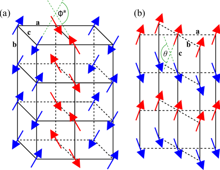
Figure 6: (Color online) Schematic views of the two exotic spin orders realized by the 3D KK model at large Hund’s exchange $\eta>0.2$: (a) striped-AF order in the $ab$ plane, with AF order along the $c$ axis and angle $\phi^{a}$ between the NN spins along the $a$ axis; (b) spin order realized in the canted-$A$-AF phase with FM order in $ab$ planes and spin canting angle $\theta$ along the $c$ axis. The regions of stability of these phases are shown in Fig. 4 by dark gray (orange) shading.

Otherwise, the phase diagram of Fig. 4 contains the $G$-AF, $A$-AF and FM configurations placed similarly as in the single-site MF phase diagram of Fig. 2. The degeneracy between the left $G$-AF and $C$-AF phase is now removed, as in the bilayer KK model,Brzezicki and Oleś (2011) and this time we provide a perturbative explanation of this fact in Sec. IV.3. Similarly to the bilayer phase diagram, the PVB phase connects with the left $G$-AF phase by the intermediate PVB-AF configuration, but due to the presence of the right $G$-AF phase we have also the right PVB-AF phase. One can summarize that the whole bottom part of the phase diagram up to $\eta\approx 0.085$ contains only smooth (second order) phase transitions when $E_{z}$ is varied. Before deriving the effective spin models for the new magnetic configurations found in the 3D KK model we will look more closely at the phase transitions along two cuts in the phase diagram of Fig. 4: (i) connecting the $A$-AF and FM phases through the canted-$A$-AF phase (Sec. III.3), and (ii) from the striped-AF to the $G$-AF phase (Sec. III.4).

III.3 From the $A$-AF to FM phase

First, we consider the negative crystal-field splitting $E_{z}=-0.5J$ — for this representative value the order changes first from the $A$-AF into the canted-$A$-AF phase, and next into the FM phase when Hund’s exchange $\eta$ increases. We selected the chain cluster of Fig. 3(b) to study these phase transitions as the spin order in the $ab$ planes does not change. The changes of spin order along the $c$ axis are captured by the cosine of the spin canting angle $\theta$ along the $c$ axis and the total magnetization $|s|$, defined in the following way:

$$\cos\theta = \frac{1}{s^{2}}\left(s_{1}^{x}s_{2}^{x}+s_{1}^{z}s_{2}^{z}\right),$$ (15)

$$|s| \equiv \sqrt{\left(s^{x}\right)^{2}+\left(s^{z}\right)^{2}},$$ (16)

and displayed in Figs. 7(a) and 7(b). For the AF configuration (in the $A$-AF phase) one finds $\theta=\pi$ ($\cos\theta=-1$), while for the FM order $\theta=0$ ($\cos\theta=1$). In the canted-$A$-AF phase $\cos\theta$ interpolates smoothly between these two limiting values. Figure 7(b) shows that the spin order parameter $|s|$ is gradually reduced and the QF increase when $\eta$ decreases and the $A$-AF phase is approached, but even in the $A$-AF phase the spin order is almost classical with $|s|\simeq 0.5$. Indeed, the QF in the $A$-AF phase with all the bonds in $ab$ planes being FM are expected to be considerably reduced from the 2D Heisenberg antiferromagnet, as shown in the spin-wave theory.Raczkowski and Oleś (2002) In the canted-$A$-AF phase the slope of $|s|$ is the largest and the QF almost saturate when the spins have rotated completely to the $A$-AF phase.

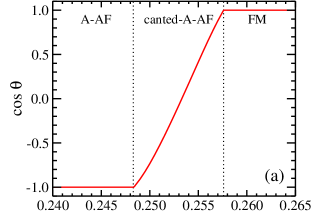
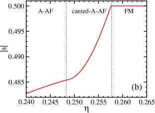
Figure 7: (Color online) Evolution of the magnetic order for increasing $\eta$ at $E_{z}=-0.5J$: (a) cosine of the canting angle $\theta$ (15), and (b) total magnetization $|s|$ (16); both in the $A$-AF, canted-$A$-AF and FM phases from left to right. Quantum phase transitions are indicated by vertical dotted lines.

The spin correlations,

$$C_{s}^{c}(d)=\langle{\bf S}_{1}\!\cdot\!{\bf S}_{1+d}\rangle\,,$$ (17)

along the $c$ axis for the NN, NNN and 3NN (distance $d=1,2,3$) are shown in Fig. 8(a), for the same path in the parameter space as in Fig. 7. The NN and 3NN correlations confirm that the order along the $c$ axis changes from the AF to FM one in a continuous way, with spin correlations passing through zero. The NNN spin correlation stays FM and is almost constant in the entire range of $\eta$. This peculiar behavior will be explained by an effective perturbative spin Hamiltonian in Sec. IV.2.

Figure 8(b) presents the spin-orbital covariances: the on-site ones,

$$r_{i}^{\gamma}=v_{i}^{z,\gamma}-s_{i}^{z}t_{i}^{\gamma}\,,$$ (18)

considered here only for the $z$ spin component $s_{i}^{z}$, and the bond covariances,

$$R^{c}\left(d\right)=\left\langle({\bf S}_{1}\!\cdot\!{\bf S}_{1+d})\,\tau_{1}^{c}\tau_{1+d}^{c}\right\rangle-\left\langle{\bf S}_{1}\!\cdot\!{\bf S}_{1+d}\right\rangle\left\langle\tau_{1}^{c}\tau_{1+d}^{c}\right\rangle\,,$$ (19)

for the NN ($d=1$) and for further neighbor ($d=2,3$) operators in the chain cluster of Fig. 3(b). As one expects, in the FM phase all the covariances vanish and the factorization of spin and orbital operators is exact.

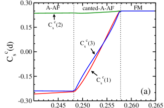
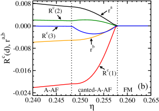
Figure 8: (Color online) Evolution of spin and orbital correlations along the $c$ axis at distance $d$, for $E_{z}=-0.5J$ and increasing $\eta$: (a) spin correlation functions $C_{s}^{c}(d)$ (17), and (b) on-site $r^{a(b)}$ (18) and bond $R^{c}(d)$ (19) spin-orbital covariances, as obtained in the $A$-AF, canted-$A$-AF and FM phase. Quantum phase transitions are indicated by vertical dotted lines.

In the canted-$A$-AF phase the slopes of the covariances are the steepest. The $R^{c}(1)$ function is the one of the largest magnitude meaning that the spin-orbital entanglement on the NN bondsOleś et al. (2006) is high. In contrast to that, the covariances $R^{c}(d)$ are close to zero for $d>1$, but $R^{c}(3)$ as the only one becomes more significant in the canted-$A$-AF phase, indicating that this phase can be governed by longer range spin interactions accompanied by orbital fluctuations. The on-site covariances behave in a monotonous way and reach relatively small absolute values meaning that they are not of the prime importance in the considered phases.

III.4 From the striped-AF to $G$-AF phase

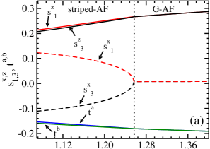
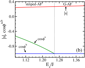
Figure 9: (Color online) Evolution from the striped-AF to $G$-AF phase at $\eta=0.22$: (a) spin $s_{1,3}^{x(z)}$ and orbital $t^{a(b)}$ order parameters, and (b) total magnetization $|s|$ (16) and cosines of spin angles $\phi^{a}$ and $\phi^{b}$, see Fig. 6(a). Quantum phase transition is indicated by vertical dotted lines.

Another exotic type of magnetic order found in the 3D KK model is the striped-AF phase. This phase can evolve smoothly towards the ordinary $G$-AF Néel order when $E_{z}$ increases. Here we use the plaquette cluster of Fig. 3(a) as the spin order in the $ab$ planes changes. In Fig. 9(a) we present the evolution of the order parameters near this transition at $\eta=0.22$. The orbital order parameters $\{t^{a},t^{b}\}$ confirm breaking of the $a$-$b$ symmetry in the striped-AF phase where they take slightly different values; this difference vanishes at the phase transition. In the magnetic sector we can distinguish four spin sublattices, see Fig. 6(a), two of which are not related by a spin inversion. To show the full complexity of the spin order we present spin averages on sites $i=1,3$ and both spin components $\alpha=x,z$. The behavior of curves confirms the striped character of the magnetic order in the striped-AF phase, vanishing at the transition point.

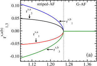
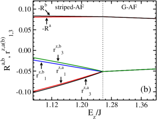
Figure 10: (Color online) Evolution of covariances from the striped-AF to $G$-AF phase at $\eta=0.22$ under increasing $E_{z}/J$ in the $ab$ planes: (a) on-site spin-orbital covariances (18) for the $x$ spin component, $r_{1(3)}^{x,a}$ and $r_{1(3)}^{x,b}$, and (b) on-site spin-orbital covariances (18) for the $x$ spin component, $r_{1(3)}^{z,a}$ and $r_{1(3)}^{z,b}$ (18), together with bond spin-orbital covariances $R^{a,b}$ (19). Quantum phase transitions are indicated by vertical dotted lines.

The quantities derived from the original order parameters, the cosines of the angle between the neighboring spins along the $a$ and $b$ axis, $\phi^{a(b)}$, and the total magnetization $|s|$, are shown in Fig. 9(b). The behavior of $\cos\phi^{a}$ and $\cos\phi^{b}$ confirms the AF order along the $b$ axis independent of $E_{z}$, while in the $a$ direction the angle $\phi^{a}$ changes at the phase transition (at $E_{z}=1.27J$) from around $2\pi/3$ to $\pi$. After the transition the cosines remain equal as expected in the isotropic AF phase. The total magnetization $|s|$ is almost constant, increasing monotonically when $E_{z}$ grows, showing that the essential physics of the striped-AF phase lies in the spin angles, although its relatively low starting value means that the striped-AF phase is affected by strong spin quantum fluctuation that weaken AF order.

In Figs. 10(a) and 10(b) we present the on-site and bond spin-orbital covariances for the same parameter range as in Fig. 9. The bond covariance $R^{\gamma}$ for a square cluster of Fig. 3(a) is defined as

$$R^{\gamma}=\left\langle({\bf S}_{1}\!\cdot\!{\bf S}_{1+\gamma})\tau_{1}^{\gamma}\tau_{1+\gamma}^{\gamma}\right\rangle-\left\langle{\bf S}_{1}\!\cdot\!{\bf S}_{1+\gamma}\right\rangle\left\langle\tau_{1}^{\gamma}\tau_{1+\gamma}^{\gamma}\right\rangle,$$ (20)

with $\gamma=a,b$. The striped-AF phase exhibits relatively large on-site entanglement in the $x$ spin component, vanishing in the $G$-AF phase, see Fig. 9(a). In contrast, the entanglement in the $z$ spin component persists in the $G$-AF phase, see Fig. 9(b). For the $x$ component the dominating covariances are the ones for the $b$ axis and for the $z$ component those along the $a$ axis. The fact that the $z$ covariances remain finite in the $G$-AF phase is somewhat surprising as one could expect that this phase with no frustration and almost fully polarized FO configuration could be trivially factorized into spin and orbital wave functions. This expectation based on the previous experienceOleś (2012) turns out to be incorrect and we show in Sec. IV.3 that high order orbital fluctuation are essential for stabilizing the AF order along the $c$ axis in this phase.

III.5 Orbital fluctuations

To estimate the strength of the orbital fluctuations in the 3D KK model one can evaluate the total orbital moment, defined in a similar way as the total magnetic moment of Eq. (16), i.e.,

$$|\tau|\equiv\frac{1}{2}\sqrt{\langle\sigma^{z}\rangle^{2}+\langle\sigma^{x}\rangle^{2}}=\frac{2\sqrt{3}}{3}\sqrt{(t^{a})^{2}+(t^{b})^{2}+t^{a}t^{b}}.$$ (21)

We investigate its value for a representative cut in the phase diagram of Fig. 4, taking $\eta=0.13$, a realistic value for KCuF₃,Oleś et al. (2005) and for $-2J<E_{z}<1.5J$ within the cluster MF and the single-site MF approximation, see Fig. 11. As expected, for algebraic reasons the orbital moment (21) in the latter approach is trivial – $|\tau|=0.5$ for all values of $E_{z}$. On the contrary, the moment $|\tau|$ found in the cluster MF is reduced from the above maximal classical value in all phases except for the $A$-AF phase where this reduction is marginal. Quantum phase transitions for increasing $E_{z}$ are marked either by discontinuities in $|\tau|$ (first order transitions) or by discontinuities in the derivative of $|\tau|$ (second order transitions).

The reduction of $|\tau|$ is most pronounced in the ortho-$G$-AF, where orbital QF couple to spins, and in the PVB-AF phase where the continuous orbital phase transition takes place but still it does not exceed $20\%$. We observe that the orbital order in the 3D KK model is robust and stable against weak QF in all phases. This result follows from the rather classical directional nature of $e_{g}$ orbitals which leads to the reduction of QF in the orbital space.van den Brink et al. (1999) The orbital order found here in the entire phase diagram justifies the perturbative expansions in the orbital sector which are used in Sec. IV to derive effective spin models. We note that this case is different from $t_{2g}$ orbitals, where orbital liquid was found both for the perovskite latticeKhaliullin and Maekawa (2000) and for the frustrated triangular lattice Normand and Oleś (2008) for the occupancy of one electron per site.

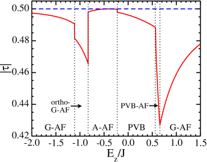
Figure 11: (Color online) Orbital moment $|\tau|$ (21) found in the cluster MF approximation at the horizontal cut of the phase diagram of Fig. 4 for $\eta=0.13$ and increasing $E_{z}$ (solid line). Quantum fluctuations reduce $|\tau|$ from the classical value of $0.5$ found in the single-site MF (dashed line). Quantum phase transitions are indicated by vertical dotted lines.

IV Effective spin models

In this Section we describe effective spin models explaining the origin of the exotic magnetic phases. Each model is obtained by perturbative expansion around the ground state with orbital order stabilized by the dominant orbital Hamiltonian ${\cal H}_{0}$. The expansion eliminates the orbital degrees of freedom yielding an effective spin Hamiltonian $H_{s}$ having the ground state with the exotic magnetic order.

IV.1 The ortho-$G$-AF phase

We begin with the exotic magnetic order found in the ortho-$G$-AF phase shown in Fig. 5 and derive an effective spin model for this phase following the same ideas as those employed in the 2D KK model (see Ref. Brzezicki et al., 2012). The idea is to use the standard quantum perturbation theory with degeneracy for the orbital sector of the KK Hamiltonian. We can divide the Hamiltonian given by Eq. (2) into the unperturbed part ${\cal H}_{0}$ and perturbation ${\cal V}$ in the following way:

$${\cal H}_{0} \equiv -J\varepsilon_{z}\sum_{i}\tau_{i}^{c}\,,$$ (22)

$${\cal V} \equiv {\cal H}-{\cal H}_{0}\,,$$ (23)

where for simplicity we use a dimensionless parameter,

$$\varepsilon_{z}\equiv\frac{E_{z}}{J}.$$ (24)

This can serve as a starting point for the perturbative treatment for large $|E_{z}|>J$. For negative $E_{z}$ (from now on in units of $J$) the ground state $\left|0\right\rangle$ of ${\cal H}_{0}$ is the state with all $z$ orbitals occupied by the holes, i.e.,

$$\forall i:\quad\tau_{i}^{c}\left|0\right\rangle=-\frac{1}{2}\left|0\right\rangle\,,$$ (25)

with energy per site $\varepsilon_{0}=\frac{1}{2}J\varepsilon_{z}$. Following the quantum perturbation theory we can construct the effective spin Hamiltonian $H_{s}$ using the expansion in powers of $\varepsilon_{z}^{-1}$:

$$H_{s}=N\varepsilon_{0}+\left\langle 0\right|{\cal V}\left|0\right\rangle-\sum_{n\not=0}\frac{|\left\langle n\right|{\cal V}\left|0\right\rangle|^{2}}{{\cal E}_{n}}+O\left(\varepsilon_{z}^{-2}\right)\,,$$ (26)

where all the overlaps are taken between the orbital states leaving the spin operators alone, ${\cal E}_{n}=\left|E_{n}-E_{0}\right|$ is the excitation energy in the physical units ($\propto J\varepsilon_{z}$), and $N$ is the number of sites. Knowing the definition of the orbital operators $\tau_{i}^{\gamma}$ Eq. (5), we can easily calculate the desired orbital overlaps. The first order gives, up to the constant term,

$$H_{s}^{(1)}=Jg_{ab}^{(1)}\sum_{i,\gamma=a,b}\left({\bf S}_{i}\cdot{\bf S}_{i+\gamma}\right)+Jg_{c}^{(1)}\sum_{i}\left({\bf S}_{i}\cdot{\bf S}_{i+c}\right)\,,$$ (27)

where $g_{ab}^{(1)}=\left(-3r_{1}+4r_{2}+r_{4}\right)/2^{5}$, $g_{c}^{(1)}=\left(r_{2}+r_{4}\right)/2$ are the in-plane and interplane coupling constants. Note that $g_{c}^{(1)}$ is positive in the whole physical range of $\eta$, while $g_{ab}^{(1)}$ is changing sign at $\eta_{0}\approx 0.1547$. If the first order term $H_{s}^{(1)}$ alone were the only spin interaction, then $\eta_{0}$ would be the point of a quantum phase transition between the $G$-AF and $A$-AF phases. However, we have found that these two phases are separated by a stripe of the exotic ortho-$G$-AF order.

Since $H_{s}^{(1)}$ vanishes at $\eta_{0}$ and therefore the first order in-plane interactions can be arbitrarily weak around $\eta_{0}$, it is necessary to go to higher order terms of the perturbative expansion to determine the in-plane interactions leading to the exotic magnetic order. In the second order the sum runs over all excited orbital states, but from the superexchange terms, Eqs. (2) and (3), one observes that ${\cal V}$ has non-zero overlap only with states either with one or with two orbitals being excited on the considered NN bond. This brings us to the second order correction of the form:

$$H_{s,ab}^{(2)}=\frac{Jg^{(2)}}{|\varepsilon_{z}|}\sum_{\left\langle\left\langle ij\right\rangle\right\rangle_{ab}}\!\left({\bf S}_{i}\cdot{\bf S}_{j}\right)-\frac{Jg^{(2)}}{2|\varepsilon_{z}|}\sum_{\left\langle\left\langle\left\langle ij\right\rangle\right\rangle\right\rangle_{ab}}\!\left({\bf S}_{i}\cdot{\bf S}_{j}\right),$$ (28)

with $g^{(2)}=3\left(r_{1}+2r_{2}+3r_{4}\right)^{2}/2^{10}$. Here $\langle\langle ij\rangle\rangle_{ab}$ and $\langle\langle\langle ij\rangle\rangle\rangle_{ab}$ denote pairs of next NN (NNN) and third NN (3NN) sites, respectively, in the $ab$-plane (for details of this deriviation see Appendix A). The second order expansion also yields an $\varepsilon_{z}^{-1}$ correction to the NN interaction strength $g_{ab}^{(1)}$, but this only moves the transition point $\eta_{0}$ and does not change the magnetic order.

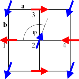
Figure 12: (Color online) Schematic view of the order imposed by the Hamiltonian (28) in the $ab$ plane. Interactions between NNN spins 1 and 3 (and equivalent) are AF, between 3NN 1 and 4 are FM, but they vanish for NN spins 1 and 2, leaving the angle $\varphi$ undetermined.

One can easily see that the ground state of the Hamiltonian (28) consists of two antiferromagnets on two interpenetrating sublattices of the square lattice, stabilized by the NNN AF Heisenberg interaction on each sublattice. Its ground state has long-range AF order renormalized by large QF. The additional 3NN FM interaction makes this AF state more classical and closer to the Néel order by suppressing partly QF. In the absence of NN coupling at $\eta_{0}$, the two AF states on sublattice are uncorrelated and the angle $\varphi$ between the respective AF order parameters remains undetermined, as shown in Fig. 12. Such ground state is similar to the ortho-$G$-AF state of Fig. 5 with AF interaction along the $c$ axis governed by $g_{c}^{(1)}$, but we still have to find the reason why the magnetic moments in two antiferromagnets prefer to be perpendicular to each other.

To answer this question we have to go to the third order of the perturbative expansion given by

$$H_{s}^{(3)}=\sum_{n\not=0}\sum_{m\not=0}\left\langle 0\right|{\cal V}\left|n\right\rangle\frac{1}{{\cal E}_{n}}\left\langle n\right|{\cal V}\left|m\right\rangle\frac{1}{{\cal E}_{m}}\left\langle m\right|{\cal V}\left|0\right\rangle.$$ (29)

After long but elementary calculations, presented in more detail in Appendix A, and under the assumption that the order shown in Fig. 12 exhibits only weak QF (see Ref. Brzezicki et al., 2012 for the arguments supporting this statement in the 2D model based on the spin-wave theory, which apply even more here in higher dimension) we obtain a classical expression for the energy per site related with the angle $\varphi$,

$$\varepsilon_{\perp}^{(3)}\approx J\frac{3^{5}}{2^{21}\varepsilon_{z}^{2}}\,(r_{1}+r_{4})\left(r_{1}\!+2r_{2}\!+3r_{4}\right)^{2}\cos^{2}\varphi\,.$$ (30)

This expression arises from a third-order four-spin interaction. As we can easily see, it is minimized by $\varphi=\pi/2$ which implies the perpendicularity of the NN spins. This finally explains the origin of the ortho-$G$-AF spin order.

IV.2 The canted-$A$-AF phase

To explain the exotic magnetic order found in the canted-$A$-AF phase, displayed in Fig. 6(b) and described in Sec. III.3, we derive an effective spin model for this phase near the orbital degeneracy at $E_{z}=0$ in a similar way as described above for the the ortho-$G$-AF phase. This time the starting unperturbed orbital Hamiltonian stabilizes the AO order,

$${\cal H}_{0}^{x}=J\varepsilon_{x}\sum_{\gamma=a,b}\sum_{{\left\langle i,j\right\rangle\parallel\gamma}}\sigma_{i}^{x}\sigma_{j}^{x},$$ (31)

where we gather all the $\sigma_{i}^{x}\sigma_{j}^{x}$ terms from the full KK Hamiltonian ${\cal H}$ in Eq. (2) (plus all constant terms which are not relevant and omitted here). This sets the coupling constant in Eq. (31) as

$$\varepsilon_{x}\equiv\frac{3}{2^{7}}\left(3r_{1}+r_{4}\right).$$ (32)

The perturbation is all the rest: ${\cal V}^{x}={\cal H}-{\cal H}_{0}^{x}$. The ground state of ${\cal H}_{0}^{x}$ is a classical configuration with the alternating eigenstates $\sigma_{i}^{x}$. This order is consistent with the cluster MF results showing that the canted-$A$-AF is an AO phase, just like the neighboring $A$-AF and FM phases.

The effective spin Hamiltonian $H_{s}$ can be constructed using the formal expansion of Eq. (26). In the zeroth order we get the ground state energy of ${\cal H}_{0}^{x}$, and in the first order the spin Hamiltonian:

$$H_{s}^{(1)}=-Jg_{ab}^{(1)}\sum_{i,\gamma=a,b}\left({\bf S}_{i}\cdot{\bf S}_{i+\gamma}\right)+Jg_{c}^{(1)}\sum_{i}\left({\bf S}_{i}\cdot{\bf S}_{i+c}\right),$$ (33)

with $g_{ab}^{(1)}\!=7(-8r_{2}+7r_{1}-r_{4})/2^{5}$, $g_{c}^{(1)}\!=(2r_{2}-r_{1}+r_{4})/2^{3}$. The NN interaction along the $c$ axis $g_{c}^{(1)}(\eta)$ is changing sign at $\eta_{0}^{x}\simeq 0.236$. This agrees well with the AF-FM crossover in the $c$ axis taking place in the canted-$A$-AF phase that separates the $A$-AF and FM phases for $\eta$ close to $\eta_{0}^{x}$. The NN interaction in the $ab$ planes $g_{ab}^{(1)}$ is FM in this region. Since the first order interaction along the $c$ axis can be made arbitrarily weak near $\eta_{0}^{x}$, we have to go to higher orders to describe interactions between different $ab$ planes.

In the second order ${\cal V}$ can produce two types of excited states: (i) with a single orbital rotated by $\pi/2$ in the $ab$ plane, or (ii) with a rotated pair of neighboring orbitals. This leads to two type of terms in the interplanar Hamiltonian,

$$H_{s,c}^{(2)}=-\frac{Jg_{c}^{(2)}}{8\varepsilon_{x}}\!\sum_{i}\left({\bf S}_{i}\!\cdot\!{\bf S}_{i+c}\right)-\frac{Jg_{cc}^{(2)}}{8\varepsilon_{x}}\sum_{i}\left({\bf S}_{i-c}\!\cdot\!{\bf S}_{i+c}\right),$$ (34)

with $g_{c}^{(2)}\!=\{\frac{2}{3}\left(r_{1}^{2}-r_{4}^{2}\right)-(r_{2}+r_{4})^{2}\}/2^{6}+\frac{1}{12}\varepsilon_{z}(r_{2}+r_{4})$, and $g_{cc}^{(2)}=(r_{2}+r_{4})^{2}/2^{7}$ (for more details see Appendix B). The NN Heisenberg interaction $g_{c}^{(2)}$ renormalizes again the first order term $g_{c}^{(1)}$, modifying slightly the value of $\eta_{0}^{x}$ where the NN coupling changes sign and makes it dependent on $E_{z}$. The $E_{z}$-dependence of the crossover from the $A$-AF to FM phase is consistent with the phase diagram in Fig. 4. The NNN interaction $g_{cc}^{(2)}$ is FM in agreement with the FM NNN correlations in the canted magnetic order shown in Fig. 6(b) and supported by the numerical result in Fig. 8(a). The nontrivial canting angle $\theta$, interpolating between $\theta=\pi$ and $\theta=0$ when passing from the $A$-AF to FM phase, remains undetermined and we must proceed to the third order of the perturbative expansion, see Appendix B.

The perturbative expansion up to third order leads to the classical expression for the ground state energy:

$$\frac{E_{0}(\theta)}{J}=\frac{\cos\theta}{4}\!\left\{\!g_{c}^{(1)}\!-\!\frac{1}{8\varepsilon_{x}}g_{c}^{(2)}\!+\!O\left(\frac{1}{\varepsilon_{x}^{2}}\right)\!\right\}\!+\!\frac{\cos^{2}\theta}{32}\frac{1}{\varepsilon_{x}^{2}}g_{c}^{(3)},$$ (35)

and we write

$$E_{0}(\theta)\equiv JA(\eta)\cos\theta+JB(\eta)\cos^{2}\theta\,.$$ (36)

Since $B(\eta)>0$, the energy has a nontrivial minimum at $\theta_{0}$ given by the equation:

$$\cos\theta_{0}=\left\{\begin{array}[]{ll}-1&\quad{\rm for}\quad\hskip 5.69046ptA(\eta)<-\frac{1}{2}B(\eta)\\ -2\frac{A(\eta)}{B(\eta)}&\quad{\rm for}\quad\left|A(\eta)\right|<\frac{1}{2}B(\eta)\\ 1&\quad{\rm for}\quad\hskip 5.69046ptA(\eta)>\frac{1}{2}B(\eta).\end{array}\right.$$ (37)

This reproduces well the behavior of $\cos\theta$ obtained via the cluster MF method, see Fig. 7(a).

IV.3 The $G$-AF versus $C$-AF spin order

Here we derive an effective spin Hamiltonian around the FO ordered state with $x$ orbitals occupied by holes to explain the energy difference between the $G$-AF and $C$-AF phase, favoring the $G$-AF order in the cluster MF approach, see Fig. 4. As in Sec. IV.1, we can divide the Hamiltonian given by Eq. (2) into the unperturbed part ${\cal H}_{0}$ (22) and the perturbation ${\cal V}$ consists of intersite terms in the $ab$ planes (${\cal V}_{ab}$) and along the $c$ axis (${\cal V}_{c}$),

$${\cal V}=J({\cal V}_{ab}+{\cal V}_{c})\,.$$ (38)

They are given as follows:

$${\cal V}_{ab}=-\frac{1}{2}\sum_{i,\gamma=a,b}H_{i,i+\gamma}^{\gamma}\,,\hskip 8.5359pt{\cal V}_{c}=-\frac{1}{2}\sum_{i}H_{i,i+c}^{c}\,.$$ (39)

For positive $E_{z}$ the ground state $\left|0\right\rangle$ of ${\cal H}_{0}$ is the state with all $x$ orbitals occupied, i.e.,

$$\forall i:\quad\tau_{i}^{c}\left|0\right\rangle=\frac{1}{2}\left|0\right\rangle,$$ (40)

with energy $E_{0}=-\frac{1}{2}J\varepsilon_{z}$ per site. Using Eq. (26) we construct the effective spin Hamiltonian $H_{s}$ as a power expansion in ${\cal V}$. Note that the ground state $\left|0\right\rangle$ is an eigenstate of ${\cal V}_{c}$ to zero eigenvalue; for this reason ${\cal V}_{c}$ gives no contribution to $H_{s}$ up to second order in ${\cal V}$ and the interplane interactions appear as $\varepsilon_{z}^{-2}$ terms.

The effective spin Hamiltonian $H_{s}$ up to second order in ${\cal V}$ can be calculated in the same way as in Sec. IV.1 and contains the same spin interactions,

$$H_{s} = J\left\{g^{(1)}\!+O\left(\varepsilon_{z}^{-1}\right)\!\right\}\!\sum_{\left\langle ij\right\rangle_{ab}}\!\left({\bf S}_{i}\!\cdot\!{\bf S}_{j}\right)+\frac{Jg^{(2)}}{\varepsilon_{z}}\!\!\!\sum_{\left\langle\left\langle ij\right\rangle\right\rangle_{ab}}\!\!\!\left({\bf S}_{i}\!\cdot\!{\bf S}_{j}\right)$$ (41)

$$\!- \frac{Jg^{(2)}}{2\varepsilon_{z}}\!\!\sum_{\left\langle\left\langle\left\langle ij\right\rangle\right\rangle\right\rangle_{ab}}\left({\bf S}_{i}\cdot{\bf S}_{j}\right)+O\left(\varepsilon_{z}^{-2}\right),$$

$g^{(1)}=3(4r_{2}-r_{1}+3r_{4})/2^{5}$, $g^{(2)}=3(2r_{2}+r_{4}-r_{1})^{2}/2^{10}$, and where all bonds are in the $ab$ planes. Again, one can think of an ortho-$G$-AF phase similar to the one obtained in the limit of $E_{z}\to-\infty$ for $\eta$ close to $\eta_{0}$ where the NN interaction $g^{(1)}$ vanishes (in this case $\eta_{0}\simeq 0.2915$) but this is not our aim here — we search for an effective description of the interplane interactions.

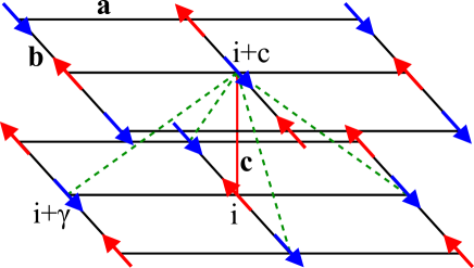
Figure 13: (Color online) Schematic view of the $G$-AF spin order on two $ab$ planes of 3D cubic lattice stabilized by the third-order FM NNN Heisenberg interactions between sites $i+\gamma$ and $i+c$ shown by dashed (green) lines (see Eq. (43)). The NN FM interactions between $i$ and $i+c$, shown by vertical (red) line, are frustrated in the $G$-AF phase.

Looking at the third order correction to $H_{s}$ given in Eq. (29) and at the form of ${\cal V}_{c}$ we can see that the interplane part of the third order correction $H_{s,c}^{(3)}$ has the following structure:

$$H_{s,c}^{(3)}=\sum_{n\not=0}\left\langle 0\right|{\cal V}_{ab}\left|n\right\rangle\frac{1}{{\cal E}_{n}}\left\langle n\right|{\cal V}_{c}\left|n\right\rangle\frac{1}{{\cal E}_{n}}\left\langle n\right|{\cal V}_{ab}\left|0\right\rangle.$$ (42)

This can be greatly simplified if we take into account two facts: (i) ${\cal V}_{ab}$ can excite only single orbitals or pair of neighboring orbitals so the sum over $n$ turns into the sum over excited sites $i$, and (ii) ${\cal V}_{c}$ is non-zero only around the excited orbitals. The final form of $H_{s,c}^{(3)}$ can be obtained using some identities for spin products and assuming that the spins form classical AF state in the $ab$ planes (see Appendix C). Of course, this is not exact because we neglect QF but these should be small in the 3D long-range ordered magnetic configuration being either $G$-AF or $C$-AF. The final formula for interplane interactions is:

$$H_{s,c}^{(3)} = -J\,\frac{9\delta_{r}}{2^{12}\varepsilon_{z}^{2}}\sum_{i}\Big{\{}g_{c}^{(3)}\left({\bf S}_{i}\cdot{\bf S}_{i+c}\right)$$ (43)

$$+ g_{ab}^{(3)}\sum_{\gamma}\left({\bf S}_{i+c}\cdot{\bf S}_{i+\gamma}\right)\Big{\}}\,,$$

with $g_{c}^{(3)}=r_{1}\left(r_{1}-r_{4}\right)$ and $g_{ab}^{(3)}=\frac{1}{4}\left(r_{1}+r_{4}\right)\left(3r_{1}-r_{4}\right)$ containing NN and NNN Heisenberg bonds both favoring ferromagnetism ($\delta_{r}$ takes only non-negative values).

This could lead to frustration as the NN bonds favor the $C$-AF state while the NNN bonds prefer the $G$-AF one, but one can easily check that the number of NNN bonds per site is four times larger than that of NN bonds (see Fig. 13). If we take into account this factor of $4$ comparing the coupling constants $g^{(3)}_{c}$ and $g^{(3)}_{ab}$ of the NN and NNN interactions we obtain:

$$4g_{ab}^{(3)}-g_{c}^{(3)}=4\frac{1+\eta\left(1-4\eta\right)}{\left(3\eta^{2}+2\eta-1\right)^{2}}>0$$ (44)

in the physical range of $\eta\in[0,1/3)$. This finally explains why the $G$-AF phase is favored over the $C$-AF phase, as long as we go beyond the single-site MF approximation which cannot capture the subtle third-order orbital fluctuations (compare Figs. 2 and 4).

IV.4 The striped-AF phase

In Sec. III.4 we summarized cluster MF results for the striped-AF phase and the continuous phase transition between the striped-AF and $G$-AF phases. These results show in particular that, unlike all other exotic phases, the striped phase has relatively large QF in both the orbital and the spin sector. Nevertheless, we attempt explaining its origin by an effective spin model keeping in mind qualitative character of our analysis.

The perturbative expansion follows the same lines as in Sec. IV.3. We assume that $E_{z}>0$ and the unperturbed ground state $|0\rangle$ is fully polarized by $E_{z}$, see Eq. (40). This is not an unreasonable starting approximation, because in Fig. 9(a) we find $t^{c}=\langle\tau^{c}_{i}\rangle\approx 0.38$ in the striped phase, i.e., only about $12\%$ of orbitals are flipped with respect to the fully polarized state $|0\rangle$. We believe that it is still justified to make a perturbative expansion in the orbital sector around the FO$x$ state. We proceed with the expansion in the same way as in Sec. 9, but here we assume AF order along the $c$ axis and focus on the $ab$ planes only.

Up to second order the effective Hamiltonian is given by Eq. (41) which can be rewritten in a more compact form,

$$H_{s} = J_{1}\sum_{\left\langle ij\right\rangle}\left({\bf S}_{i}\!\cdot\!{\bf S}_{j}\right)$$ (45)

$$+ J_{2}\left\{\sum_{\left\langle\left\langle ij\right\rangle\right\rangle}\left({\bf S}_{i}\!\cdot\!{\bf S}_{j}\right)-\frac{1}{2}\sum_{\left\langle\left\langle\left\langle ij\right\rangle\right\rangle\right\rangle}\left({\bf S}_{i}\!\cdot\!{\bf S}_{j}\right)\right\},$$

with both $J_{1},J_{2}>0$ in the physically interesting range of $\eta$ and $E_{z}$. The first two terms are the same as in the $J_{1}-J_{2}$ model whose ground state is AF when $J_{1}\gg J_{2}$ and collinear when $J_{1}\ll J_{2}$. The extra 3NN FM coupling is consistent with the NNN AF coupling, hence the phase diagram of the present model should be qualitatively the same.

In a classical approximation, the phase diagram of the $J_{1}-J_{2}$ model (45) motivates an Ansatz, where

$${\bf S}_{i}\!\cdot\!{\bf S}_{i+b}={\bf S}_{i}\!\cdot\!{\bf S}_{i+c}=-\frac{1}{2}~{},$$

$${\bf S}_{i}\!\cdot\!{\bf S}_{i+a}=\frac{1}{2}\cos\phi^{a}=-\frac{1}{2}\cos\alpha,$$ (46)

with $\alpha=\pi-\phi^{a}$, see Fig. 6(a). Here the angle $\alpha$ is a variational parameter. The Ansatz breaks the symmetry between the $a$ and $b$ axes. It can describe the AF phase when $\alpha=0$, the collinear phase when $\alpha=\pi$, and the intermediate striped-AF phase when $\alpha\in(0,\pi)$. Up to an additive constant, the energy per site is

$$\varepsilon(\alpha)~{}=~{}(-J_{1}+2J_{2})\cos\alpha\,.$$ (47)

It suggests a discontinuous (first order) transition between the AF and collinear phases at $J_{1}=2J_{2}$. Thus, up to second order in the perturbative expansion, the striped phase is unstable in the classical version of the effective spin Hamiltonian $H_{s}$. However, near the critical point, where the energy $\varepsilon(\alpha)$ does not depend on $\alpha$, the ground state can be very susceptible to any perturbation from higher order terms in $H_{s}$.

Indeed, the third order term $H^{(3)}_{s}$ contains the relevant perturbation (29) of the form

$$H_{s,ab}^{(3)}=J_{3}\sum_{\left\langle ij\right\rangle\|\gamma}\left({\bf S}_{i}\cdot{\bf S}_{j}\right)\sum_{{\gamma^{\prime}\not=\gamma\atop\gamma^{\prime\prime}\not=-\gamma}}s_{\gamma^{\prime}}s_{\gamma^{\prime\prime}}\left({\bf S}_{i+\gamma^{\prime}}\cdot{\bf S}_{j+\gamma^{\prime\prime}}\right)\,,$$ (48)

where $\gamma^{\prime}$, $\gamma^{\prime\prime}$ stand for possible direction $\{a,b\}$ in the square lattice, and $s_{\pm a(}=1$, $s_{\pm b}=-1$, respectively. Including these interactions, the energy per site becomes

$$\varepsilon(\alpha)~{}=~{}(-J_{1}+2J_{2}+4J_{3})\cos\alpha~{}+~{}5J_{3}\cos^{2}\alpha\,.$$ (49)

Now the system undergoes a continuous symmetry-breaking phase transition from the AF phase ($|\alpha|=0$) to the striped phase ($|\alpha|>0$) when $J_{1}$ becomes less than $2J_{2}+14J_{3}$. This is where the quadratic term $\varepsilon_{2}$ in the Landau expansion of energy, $\varepsilon(\alpha)\approx\varepsilon_{0}+\varepsilon_{2}\alpha^{2}+\varepsilon_{4}\alpha^{4}$, becomes negative favoring a finite value of the order parameter $\alpha$. The continuous character of the transition is consistent with the cluster MF results in Fig. 9.

In conclusion, the effective classical spin model provides a qualitative explanation for the origin of the striped-AF phase. We do not present any quantitative predictions here — they would be rather poor due to large spin QF in the striped phase.

V Summary and conclusions

We have presented a rather complete analysis of the phase diagram of the 3D Kugel–Khomskii model in the framework of the cluster MF theory and effective perturbative models. It is found that spin disordered plaquette valence-bond phase is stable near the orbital degeneracy in the broad range of Hund’s exchange, resolving the existing controversy and in agreement with the earlier studies.Feiner et al. (1997, 1998) Furthermore, we managed to obtain a very transparent picture in the left part of the phase diagram of Fig. 4 (for negative crystal-field splitting), with a sequence of phase transitions occurring for increasing $\eta$ and involving two intermediate phases with exotic magnetic orders. This sequence is caused by the (first order) NN Heisenberg interactions changing their sign from AF to FM spin interaction: (i) first in the $ab$ plane, where the ortho-$G$-AF phase occurs, and (ii) next along the $c$ axis, which leads to the canted-$A$-AF configuration. In both cases we found perturbative expansions around certain orbital configurations explaining these puzzling magnetic orders by further neighbor spin interactions. In case of the ortho-$G$-AF phase the effective Hamiltonian is the same as for the 2D KK model with additional AF interactions along the $c$ axis. In the other case the intermediate configuration turned out to be essentially classical, with FM planes damping spin quantum fluctuations, and we have used this fact to construct the effective spin model around the AO configuration to explain the canted-$A$-AF ordering.

To supplement these analytical considerations we presented the plots of order parameters, correlations and spin-orbital covariances for the two cuts in the phase diagram, passing through canted-$A$-AF and striped-AF phases. They show that both phases involve spin-orbital entanglementOleś (2012) and the plots for the canted-$A$-AF phase are supported by the effective spin Hamiltonian derived for this phase. The plots for the ortho-$G$-AF phase were already given in the 2D case, Brzezicki et al. (2012) and they are rather similar for the present 3D cubic lattice (not shown).

In contrast, some of our results in the right part of the phase diagram (for positive crystal-field splitting) are more qualitative. As the last analytical result we showed the derivation of the effective spin Hamiltonian for the FO$x$ configuration which explains why the $G$-AF phase always wins over the $C$-AF order for the 3D and bilayer systems although these two phases are degenerate in the single-site MF approach. The answer was found in the third order of the perturbation expansion and it was showed that the AF order along the $c$ axis is induced by the two effects: (i) AF order in the $ab$ planes, and (ii) NNN interaction between the planes being FM. Surprisingly, this demonstrates that the right $G$-AF phase is highly spin-orbital entangled, as shown in Fig. 10 because we need third order orbital fluctuations to stabilize the spin order, and agrees with the plots of spin-orbital covariances presented for the bilayer KK model.Brzezicki and Oleś (2011) This may be the reason for a stronger divergence of the quantum corrections to the order parameter found in the spin-wave theory.Feiner et al. (1998)

Our study has shown that the striped-AF phase still requires a more sophisticated approach than the one that was implemented here. In particular, it is not clear why this phase appears only in the 3D case; we have verified that it converges to a stable solution in the 2D case, but with energy being always higher than that of either the $G$-AF or FM phase. This remains one of the open questions in the phase diagram of the 3D Kugel–Khomskii model and further studies beyond the cluster MF, such as the entanglement renormalization ansatz, Vidal (2007); *Vid08; *Cin08 are needed.

Summarizing, we have established that orbital excitations not only couple to spin fluctuations,Wohlfeld et al. (2011) but may even change the spin order in spin-orbital systems. On the example of the 3D Kugel–Khomskii model we have shown that three magnetic phases with exotic spin order arise near the crossover from AF to FM spin interactions at increasing Hund’s exchange and are triggered by entangled spin-orbital quantum fluctuations. The derived effective spin models, that include second and third neighbor spin interactions and go beyond the Heisenberg paradigm, provide good microscopic insights into these phases. At the same time, these effective interactions do not confirm the earlier suggestion Feiner et al. (1997) that the resonating valence-bond phase accompanied by the FO order of $3z^{2}-r^{2}$ orbitals along the $c$ axis could be stable instead.

The derived phase diagram could in principle describe also the $A$-AF phase observed in KCuF₃ at low temperature,Lake et al. (2005) taking realistic parameters, but the signatures of the 1D Heisenberg physics are missing. On the one hand, it supports the recent view that the Kugel-Khomskii model is incomplete and should be extended by the Goodenough processesOleś et al. (2005) and by other (lattice) degrees of freedomLee et al. (2012) to explain fully the observed physical properties of KCuF₃. On the other hand, the present study provides an experimental challenge whether the ortho-$G$-AF phase could be discovered in KCuF₃, for instance using high pressure studies.

Appendix A Spin model in the ortho-$G$-AF phase

The form of second order contribution to the effective in-plane spin Hamiltonian can be derived from Eq. (26) by calculating the matrix elements $\left\langle n\right|{\cal V}\left|0\right\rangle$ in the orbital sector. As a result we get

$$H_{s,ab}^{(2)} = \frac{J}{\varepsilon_{z}}g^{(2)}\sum_{i}\left\{\sum_{\gamma}s_{\gamma}\left({\bf S}_{i}\cdot{\bf S}_{i+\gamma}\right)\right\}^{2}$$

$$+ \frac{J}{\varepsilon_{z}}\frac{9}{2^{11}}\!\sum_{\left\langle ij\right\rangle}\left\{\left({\bf S}_{i}\cdot{\bf S}_{j}\right)(r_{1}+r_{4})+\frac{3r_{1}-r_{4}}{4}\right\}^{2},$$

where $s_{\gamma}$ is a sign factor depending on the bond’s direction $\gamma$ and originating from the definition of operators $\tau_{i}^{a(b)}$, i.e.,

$$s_{\gamma}=\left\{\begin{array}[]{ccc}1&{\rm if}&\gamma=\pm a\\ -1&{\rm if}&\gamma=\pm b\end{array}\right\},$$ (51)

and $g^{(2)}$ is defined in Section IV.1. The squared quantities in $H_{s}^{(2)}$ produce spin products of the two forms, shown in Fig. 14(a) and 14(b), which can be simplified using elementary spin identities:

$$\left({\bf S}_{i+\gamma}\cdot{\bf S}_{i}\right)\left({\bf S}_{i}\cdot{\bf S}_{i+\gamma^{\prime}}\right) = \frac{1}{4}\left({\bf S}_{i+\gamma}\cdot{\bf S}_{i+\gamma^{\prime}}\right)$$ (52)

$$+ \frac{i}{2}\,{\bf S}_{i+\gamma}\!\cdot\left({\bf S}_{i}\times{\bf S}_{i+\gamma^{\prime}}\right)\,,$$

$$\left({\bf S}_{i}\cdot{\bf S}_{i+\gamma}\right)^{2} = -\frac{1}{2}\left({\bf S}_{i}\cdot{\bf S}_{i+\gamma}\right)+\frac{3}{16}\,.$$ (53)

The latter identity simplifies the second line of $H_{s,ab}^{(2)}$ and produces $E_{z}^{-1}$ correction to the Heisenberg interactions in $H_{s}^{(1)}$, while the former one leads to the interactions between further neighbors in Eq. (28). The imaginary term in Eq. (52) is antihermitian and must cancel out with other terms in $H_{s,ab}^{(2)}$. Thus, in $H_{s,ab}^{(2)}$, we are left with the pure Heisenberg term $\left({\bf S}_{i+\gamma}\cdot{\bf S}_{i+\gamma^{\prime}}\right)$ connecting sites $i+\gamma$ and $i+\gamma^{\prime}$, being either NNN or 3NN, presented in Fig. 14(a) and 14(b), with the sign given by $s_{\gamma}s_{\gamma^{\prime}}$. Due to the double counting of the interactions the 3NN couplings in $H_{s,ab}^{(2)}$ of Eq. (28) is twice weaker than the NNN ones.

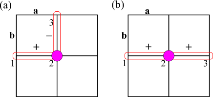
Figure 14: (Color online) Schematic views of second order corrections in the effective spin Hamiltonian: (a) effective NNN interactions, and (b) effective 3NN interaction. Red frames stand for Heisenberg bond with $\pm$ sign depending on the bond’s direction and filled (magenta) dots are the single-site orbital excitations in the ground state.

The third order correction necessary to determine the in-plane NN interaction at $\eta_{0}$ is given by Eq. (29); here we limit the sums over the excited orbital states $\left\{\left|n\right\rangle,\left|m\right\rangle\right\}$ only to the ones with orbital flips lying in the same $ab$ plane. This produces many contributions to the spin Hamiltonian but we are interested only in terms with new operator structure with respect to lower orders because the others will be just the $E_{z}^{-2}$ corrections to the already existing interactions. The terms bringing potentially new physics are the ones with three different Heisenberg bonds multiplied one after another. Such contribution is depicted in Fig. 15(a) for sites $i=1,2,3,4$ (in contrast, Fig. 15(b) shows the term bringing no new contribution to $H_{s}$) and can be transformed following the identity,

$$\left({\bf S}_{1}\!\cdot\!{\bf S}_{2}\right)\left({\bf S}_{2}\!\cdot\!{\bf S}_{3}\right)\left({\bf S}_{3}\!\cdot\!{\bf S}_{4}\right)=$$ (54)

$$\frac{1}{16}\,{\bf S}_{1}\!\cdot\!{\bf S}_{4}+\frac{1}{4}\left({\bf S}_{1}\!\cdot\!{\bf S}_{4}\right)\left({\bf S}_{2}\!\cdot\!{\bf S}_{3}\right)$$

$$- \frac{1}{4}\left({\bf S}_{1}\!\cdot\!{\bf S}_{3}\right)\left({\bf S}_{2}\!\cdot\!{\bf S}_{4}\right)+\frac{i}{8}\,{\bf S}_{1}\!\cdot\left({\bf S}_{3}\times{\bf S}_{4}\right)$$

$$+ \frac{i}{8}\,{\bf S}_{1}\!\cdot\left({\bf S}_{4}\times{\bf S}_{2}\right)+\frac{i}{8}\,{\bf S}_{1}\!\cdot\left({\bf S}_{4}\times{\bf S}_{2}\right),$$

where the cross-product terms are antihermitian and must cancel out with other terms of the same structure in $H_{s,ab}^{(3)}$. To analyze the remaining terms in Eq. (54) it is helpful to employ the almost classical nature of the AF spin order on two sublattices: (i) the first term is an AF interaction between the sublattices which is not compatible with the antiferromagnetism on sublattices that is one order of $E_{z}$ stronger, (ii) the second term favors perpendicularity of the two AF sublattices, as long as its sign is positive, which is compatible with the order on sublattices, and (iii) the third term brings no new information about the spin order.

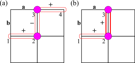
Figure 15: (Color online) Schematic view of third order corrections to $H_{s}$ (frames stand for Heisenberg bonds with $\pm$ sign depending on their direction, filled circles indicate orbital flips): (a) term bringing new physics, chain product of three bonds, (b) term doubling the results from second order expansion, interaction between spins $2$ and $3$ is squared (bond marked by a thick frame).

Putting all together, we can argue that the third order perturbative contributions in Eq. (54) can favor perpendicularity of the order parameters on two sublattice antiferromagnets. Now we have to extract all such contributions from Eq. (29)and check whether the total sign is indeed positive because otherwise our arguments would be incomplete. After lengthy but elementary calculation (see Ref. Brzezicki et al., 2012 for more details) we obtain the third order Hamiltonian, with interactions not included in lower orders of the form:

$$H_{s,ab}^{(3)} = J\,\frac{27}{2^{17}\,\varepsilon_{z}^{2}}\left(r_{1}+r_{4}\right)\left(r_{1}+2r_{2}+3r_{4}\right)^{2}$$

$$\times \sum_{\left\langle ij\right\rangle\|\gamma}\left({\bf S}_{i}\cdot{\bf S}_{j}\right)\sum_{{\gamma^{\prime}\not=\gamma\atop\gamma^{\prime\prime}\not=-\gamma}}s_{\gamma^{\prime}}s_{\gamma^{\prime\prime}}\left({\bf S}_{i+\gamma^{\prime}}\!\cdot\!{\bf S}_{j+\gamma^{\prime\prime}}\right).$$

These are the special contributions of the type shown in Fig. 15(a) taken into account here. This, in the classical limit, gives the energy $\varepsilon_{\perp}^{(3)}$ in Eq. (30) favoring perpendicular orientation of the NN spins.

Appendix B Spin model in the canted-$A$-AF phase

To calculate the second order correction to the spin Hamiltonian $H_{s}$ in the canted-$A$-AF phase we have to, as before, calculate the matrix element (overlap) $\left\langle n\right|{\cal V}^{x}\left|0\right\rangle$ in the orbital sector. Since the state $\left|n\right\rangle$ is an excited state of ${\cal H}_{0}$, the non-zero overlap can be obtained only for the part ${\cal V}^{x}$ of the interaction ${\cal V}$ that contains at least one operator $\sigma_{i}^{z}$. Assuming FM order in the $ab$ planes it can be written as,

$${\cal V}^{x} = \frac{Jr_{1}}{2^{5}}\sum_{{\left\langle ij\right\rangle\parallel\atop\gamma=a,b}}\left\{\sigma_{j}^{z}\sigma_{i}^{z}-s_{\gamma}\sqrt{3}\left(\sigma_{j}^{z}\sigma_{i}^{x}+\sigma_{j}^{x}\sigma_{i}^{z}\right)\right\}$$ (56)

$$+ \frac{J}{8}\sum_{{\left\langle ij\right\rangle\parallel\atop c}}\left\{\left(r_{1}\Pi_{t}^{(ij)}-r_{4}\Pi_{s}^{(ij)}\right)\sigma_{i}^{z}\sigma_{j}^{z}\right.$$

$$+ \left.(r_{2}+r_{4})\Pi_{s}^{(ij)}\left(\sigma_{i}^{z}+\sigma_{j}^{z}\right)\right\}-\frac{1}{2}\,E_{z}\sum_{i}\sigma_{i}^{z}\,.$$

employing the spin projectors in Eqs. (6). Now we can derive the second order Hamiltonian,

$$H_{s}^{(2)} = -\frac{J}{8\varepsilon_{x}}\sum_{i}\left\{\frac{\varepsilon_{z}}{2}+\frac{r_{2}+r_{4}}{8}\left(\frac{1}{2}-\sum_{\gamma=\pm c}{\bf S}_{i}\!\cdot\!{\bf S}_{i+\gamma}\right)\right\}^{2}$$

$$- \frac{J}{3\varepsilon_{x}}\sum_{i}\frac{1}{2^{8}}\left\{(r_{1}+r_{4})({\bf S}_{i}\cdot{\bf S}_{i+c})+\frac{3r_{1}-r_{4}}{4}\right\}^{2},$$

which can be easily transformed into Eq. (34) using the identity (52).

In the third order we are interested only in terms with three Heisenberg bonds multiplied by each other along the $c$ direction, according to Eq. (54), as all other possible products will only reproduce the results from lower orders. Such terms lead to the correction $H_{s,c}^{(3)}$ of the form:

$$H_{s,c}^{(3)}\!=\frac{Jg_{c}^{(3)}}{\varepsilon_{x}^{2}}\!\sum_{i}\!\left\{\!\left({\bf S}_{i+c}\!\cdot\!{\bf S}_{i}\right)\!\left({\bf S}_{i}\!\cdot\!{\bf S}_{i-c}\right)\!\left({\bf S}_{i-c}\!\cdot\!{\bf S}_{i-2c}\right)+{\rm H.c.}\right\},$$ (58)

with $g_{c}^{(3)}=\frac{5}{6}\left(r_{2}+r_{4}\right)^{2}\left(r_{4}+r_{1}\right)/2^{14}$. This can be further simplified using the identity (53),

$$H_{s,c}^{(3)} \!=\! J\frac{g_{c}^{(3)}}{8\varepsilon_{x}^{2}}\!\sum_{i}\left\{\left({\bf S}_{i+c}\!\cdot\!{\bf S}_{i-2c}\right)+4\left({\bf S}_{i+c}\!\cdot\!{\bf S}_{i-2c}\right)\!\left({\bf S}_{i}\!\cdot\!{\bf S}_{i-c}\right)\right.$$ (59)

$$\!-\! \left.4\left({\bf S}_{i+c}\!\cdot\!{\bf S}_{i-c}\right)\left({\bf S}_{i}\!\cdot\!{\bf S}_{i-2c}\right)\right\}.$$

Now, according to Fig. 6(b), we use the classical expressions for the spin scalar product using the canting angle $\theta$ for the odd neighbors and FM order for the even neighbors, imposed by the second order Hamiltonian of Eq. (34), i.e.,

$${\bf S}_{i}\cdot{\bf S}_{i+(2n-1)c}=\frac{1}{4}\cos\theta,\hskip 14.22636pt{\bf S}_{i}\cdot{\bf S}_{i+2nc}=\frac{1}{4}.$$ (60)

After inserting this into Eq. (59) only the first line depends on $\theta$ and gives a contribution to the classical ground state energy $E_{0}(\theta)$ of the canted-$A$-AF phase see Eq. (36).

Appendix C Spin model in the $G$-AF phase

Here we consider the $G$-AF phase with FO$x$ order for $E_{z}>0$. The third order contribution of the form given by Eq. (42) can be expressed as,

$$H_{s,c}^{(3)} \!= -J\frac{g^{(2)}\delta_{r}}{2\varepsilon_{z}^{2}}\!\sum_{i,\gamma,\gamma^{\prime}}\!s_{\gamma}s_{\gamma^{\prime}}\left({\bf S}_{i}\!\cdot\!{\bf S}_{i+\gamma}\right)\left({\bf S}_{i}\!\cdot\!{\bf S}_{i+c}\right)\left({\bf S}_{i}\!\cdot\!{\bf S}_{i+\gamma^{\prime}}\right)$$ (61)

$$\!- J\frac{9\delta_{r}}{2^{13}\varepsilon_{z}^{2}}\sum_{i,\gamma}\left\{(r_{1}+r_{4})\left({\bf S}_{i}\!\cdot\!{\bf S}_{i+\gamma}\right)+\frac{3r_{1}-r_{4}}{4}\right\}$$

$$\!\times \left({\bf S}_{i}\!\cdot\!{\bf S}_{i+c}\right)\left\{(r_{1}+r_{4})\left({\bf S}_{i}\!\cdot\!{\bf S}_{i+\gamma}\right)+\frac{3r_{1}-r_{4}}{4}\right\},$$

where $\delta_{r}=r_{1}-r_{2}$, sums over $\gamma$ and $\gamma^{\prime}$ run over the in-plane directions $\left\{\pm a,\pm b\right\}$. The first term in Eq. (61) comes from single-orbital excitations, while the second one (second and third line) — from two-orbital excitations. The interplane interactions are typically sandwiched between two in-plane bonds; these can be treated with the following spin identity:

$$\left({\bf S}_{i}\!\cdot\!{\bf S}_{i+\gamma}\right)\left({\bf S}_{i}\!\cdot\!{\bf S}_{i+c}\right)\left({\bf S}_{i}\!\cdot\!{\bf S}_{i+\gamma^{\prime}}\right)$$

$$= \frac{1}{4}\left({\bf S}_{i+c}\!\cdot\!{\bf S}_{i+\gamma}\!\right)\left({\bf S}_{i}\!\cdot\!{\bf S}_{i+\gamma^{\prime}}\!\right)-\frac{1}{4}\left({\bf S}_{i+\gamma^{\prime}}\!\cdot\!{\bf S}_{i+\gamma}\right)\left({\bf S}_{i}\!\cdot\!{\bf S}_{i+c}\right)$$

$$+ \frac{1}{4}\left({\bf S}_{i}\!\cdot\!{\bf S}_{i+\gamma}\!\right)\left({\bf S}_{i+c}\!\cdot\!{\bf S}_{i+\gamma^{\prime}}\!\right)+\frac{i}{8}\,{\bf S}_{i+\gamma}\!\cdot\!\left({\bf S}_{i+c}\times{\bf S}_{i+\gamma^{\prime}}\right)\,.$$

Under the assumption of the classical AF order in $ab$ planes, i.e., $\left({\bf S}_{i}\cdot{\bf S}_{i+\gamma}\right)\equiv-\frac{1}{4}$ for $\gamma=\pm a,\pm b$, the above identity gives the following results for the tri-quadratic spin products in $H_{s,c}^{(3)}$,

$$\sum_{\gamma,\gamma^{\prime\prime}} s_{\gamma}s_{\gamma^{\prime\prime}}\left({\bf S}_{i}\!\cdot\!{\bf S}_{i+\gamma}\right)\left({\bf S}_{i}\!\cdot\!{\bf S}_{i+c}\right)\left({\bf S}_{i}\!\cdot\!{\bf S}_{i+\gamma^{\prime\prime}}\right)$$ (63)

$$= \frac{1}{4}\sum_{\gamma}\left({\bf S}_{i+c}\!\cdot\!{\bf S}_{i+\gamma}\right)+\frac{1}{4}\left({\bf S}_{i}\!\cdot\!{\bf S}_{i+c}\right)\,,$$

and

$$\left({\bf S}_{i}\!\cdot\!{\bf S}_{i+\gamma}\right)\left({\bf S}_{i}\!\cdot\!{\bf S}_{i+c}\right)\left({\bf S}_{i}\!\cdot\!{\bf S}_{i+\gamma}\right)=-\frac{1}{16}\left({\bf S}_{i}\!\cdot\!{\bf S}_{i+c}\right)\,.$$ (64)

The biquadratic terms can be simplified using identity (52). Note that the classical AF order, $\left({\bf S}_{i}\cdot{\bf S}_{i+\gamma}\right)\equiv-\frac{1}{4}$ for $\gamma=\pm a,\pm b$, is inserted after the spin products are sorted out with spin identities (52) and (LABEL:eq:Sid3) but not before. This is an important distinction: we extract the result of higher order in-plane spin fluctuations before we freeze them out to get a simplified picture. After gathering all the interactions together we obtain $H_{s,c}^{(3)}$ in Eq. (43).

References

- Feiner et al. (1997) L. F. Feiner, A. M. Oleś, and J. Zaanen, Phys. Rev. Lett. 78, 2799 (1997).
- Kugel and Khomskii (1973) K. I. Kugel and D. I. Khomskii, JETP 37, 725 (1973).
- Kugel and Khomskii (1982) K. I. Kugel and D. I. Khomskii, Usp. Fiz. Nauk 136, 621 (1982).
- Tokura and Nagaosa (2000) Y. Tokura and N. Nagaosa, Science 288, 462 (2000).
- van den Brink et al. (2011) J. van den Brink, Z. Nussinov, and A. M. Oleś, Introduction to Frustrated Magnetism: Materials, Experiments, Theory (Springer, New York, 2011) pp. 631-672.
- Khaliullin (2005) G. Khaliullin, Prog. Theor. Phys. Suppl. 160 (2005).
- Oleś et al. (2005) A. M. Oleś, G. Khaliullin, P. Horsch, and L. F. Feiner, Phys. Rev. B 72, 214431 (2005).
- Oleś (2012) A. M. Oleś, J. Phys.: Condens. Matter 24, 313201 (2012).
- Zaanen and Oleś (1993) J. Zaanen and A. M. Oleś, Phys. Rev. B 48, 7197 (1993).
- Feiner and Oleś (1999) L. F. Feiner and A. M. Oleś, Phys. Rev. B 59, 3295 (1999).
- van den Brink et al. (1999) J. van den Brink, P. Horsch, F. Mack, and A. M. Oleś, Phys. Rev. B 59, 6795 (1999).
- Paolasini et al. (2002) L. Paolasini, R. Caciuffo, A. Sollier, P. Ghigna, and M. Altarelli, Phys. Rev. Lett. 88, 106403 (2002).
- Caciuffo et al. (2002) R. Caciuffo, L. Paolasini, A. Sollier, P. Ghigna, E. Pavarini, J. van den Brink, and M. Altarelli, Phys. Rev. B 65, 174425 (2002).
- Binggeli and Altarelli (2004) N. Binggeli and M. Altarelli, Phys. Rev. B 70, 085117 (2004).
- Deisenhofer et al. (2008) J. Deisenhofer, I. Leonov, M. V. Eremin, C. Kant, P. Ghigna, F. Mayr, V. V. Iglamov, V. I. Anisimov, and D. van der Marel, Phys. Rev. Lett. 101, 157406 (2008).
- Leonov et al. (2010) I. Leonov, D. Korotin, N. Binggeli, V. I. Anisimov, and D. Vollhardt, Phys. Rev. B 81, 075109 (2010).
- Lee et al. (2012) J. C. T. Lee, S. Yuan, S. Lal, Y. I. Joe, Y. Gan, S. Smadici, K. Finkelstein, Y. Feng, A. Rusydi, P. M. Goldbart, S. L. Cooper, and P. Abbamonte, Nat. Phys. 8, 63 (2012).
- Eremin et al. (2008) M. V. Eremin, D. V. Zakharov, H. A. K. von Nidda, R. M. Eremina, A. Shuvaev, A. Pimenov, P. Ghigna, J. Deisenhofer, and A. Loidl, Phys. Rev. Lett. 101, 147601 (2008).
- Yamada and Kato (1994) I. Yamada and N. Kato, J. Phys. Soc. Jpn. 63, 289 (1994).
- Lake et al. (2005) B. Lake, D. A. Tennant, C. D. Frost, and S. E. Nagler, Nature Materials 4, 329 (2005).
- Tennant et al. (1993) D. A. Tennant, T. G. Perring, R. A. Cowley, and S. E. Nagler, Phys. Rev. Lett. 70, 4003 (1993).
- Oleś et al. (2000) A. M. Oleś, L. F. Feiner, and J. Zaanen, Phys. Rev. B 61, 6257 (2000).
- Feiner et al. (1998) L. F. Feiner, A. M. Oleś, and J. Zaanen, J. Phys.: Condens. Matter 10, L555 (1998).
- Khaliullin and Oudovenko (1997) G. Khaliullin and V. Oudovenko, Phys. Rev. B 56, R14243 (1997).
- Normand (2009) B. Normand, Contemporary Physics 50, 533 (2009).
- Balents (2010) L. Balents, Nature 464, 199 (2010).
- Cincio et al. (2010) L. Cincio, J. Dziarmaga, and A. M. Oleś, Phys. Rev. B 82, 104416 (2010).
- Silva et al. (2003) T. N. D. Silva, A. Joshi, M. Ma, and F. C. Zhang, Phys. Rev. B 68, 184402 (2003).
- Oleś et al. (2006) A. M. Oleś, P. Horsch, L. F. Feiner, and G. Khaliullin, Phys. Rev. Lett. 96, 147205 (2006).
- Frischmuth et al. (1999) B. Frischmuth, F. Mila, and M. Troyer, Phys. Rev. Lett. 82, 835 (1999).
- Oleś et al. (2007) A. M. Oleś, P. Horsch, and G. Khaliullin, Phys. Stat. Solidi B 244, 2378 (2007).
- You et al. (2012) W.-L. You, A. M. Oleś, and P. Horsch, Phys. Rev. B 86, 094412 (2012).
- Normand and Oleś (2008) B. Normand and A. M. Oleś, Phys. Rev. B 78, 094427 (2008).
- Normand (2011) B. Normand, Phys. Rev. B 83, 064413 (2011).
- Chaloupka and Oleś (2011) J. Chaloupka and A. M. Oleś, Phys. Rev. B 83, 094406 (2011).
- Trousselet et al. (2012) F. Trousselet, A. Ralko, and A. M. Oleś, Phys. Rev. B 86, 014432 (2012).
- Goodenough (1963) J. B. Goodenough, Magnetism and the Chemical Bond (Interscience, New York, 1963).
- Kanamori (1959) J. Kanamori, J. Phys. Chem. Solids 10, 87 (1959).
- Khaliullin et al. (2004) G. Khaliullin, P. Horsch, and A. M. Oleś, Phys. Rev. B 70, 195103 (2004).
- Horsch et al. (2008) P. Horsch, A. M. Oleś, L. F. Feiner, and G. Khaliullin, Phys. Rev. Lett. 100, 167205 (2008).
- Ulrich et al. (2003) C. Ulrich, G. Khaliullin, J. Sirker, M. Reehuis, M. Ohl, S. Miyasaka, Y. Tokura, and B. Keimer, Phys. Rev. Lett. 91, 257202 (2003).
- Horsch et al. (2003) P. Horsch, G. Khaliullin, and A. M. Oleś, Phys. Rev. Lett. 91, 257203 (2003).
- Sirker et al. (2008) J. Sirker, A. Herzog, A. M. Oleś, and P. Horsch, Phys. Rev. Lett. 101, 157204 (2008).
- Sirker and Khaliullin (2003) J. Sirker and G. Khaliullin, Phys. Rev. B 67, 100408 (2003).
- Herzog et al. (2011) A. Herzog, P. Horsch, A. M. Oleś, and J. Sirker, Phys. Rev. B 83, 245130 (2011).
- Brzezicki and Oleś (2011) W. Brzezicki and A. M. Oleś, Phys. Rev. B 83, 214408 (2011).
- Brzezicki and Oleś (2012) W. Brzezicki and A. M. Oleś, J. Phys.: Conf. Series 391, 012085 (2012).
- Brzezicki et al. (2012) W. Brzezicki, J. Dziarmaga, and A. M. Oleś, Phys. Rev. Lett. 109, 237201 (2012).
- Oleś et al. (1987) A. M. Oleś, J. Zaanen, and P. Fulde, Physica B & C 148, 260 (1987).
- Oleś and Grzelka (1991) A. M. Oleś and W. Grzelka, Phys. Rev. B 44, 9531 (1991).
- Grant and McMahan (1992) J. B. Grant and A. K. McMahan, Phys. Rev. B 46, 8440 (1992).
- Feiner and Oleś (2005) L. F. Feiner and A. M. Oleś, Phys. Rev. B 71, 144422 (2005).
- Oleś (1983) A. M. Oleś, Phys. Rev. B 28, 327 (1983).
- Liechtenstein et al. (1995) A. I. Liechtenstein, V. I. Anisimov, and J. Zaanen, Phys. Rev. B 52, R5467 (1995).
- Raczkowski and Oleś (2002) M. Raczkowski and A. M. Oleś, Phys. Rev. B 66, 094431 (2002).
- Khaliullin and Maekawa (2000) G. Khaliullin and S. Maekawa, Phys. Rev. Lett. 85, 3950 (2000).
- Vidal (2007) G. Vidal, Phys. Rev. Lett. 99, 220405 (2007).
- Vidal (2008) G. Vidal, Phys. Rev. Lett. 101, 110501 (2008).
- Cincio et al. (2008) L. Cincio, J. Dziarmaga, and M. M. Rams, Phys. Rev. Lett. 100, 240603 (2008).
- Wohlfeld et al. (2011) K. Wohlfeld, M. Daghofer, S. Nishimoto, G. Khaliullin, and J. van den Brink, Phys. Rev. Lett. 107, 147201 (2011).