Weak Convergence Methods for Approximation of the Evaluation of Path-dependent Functionals

Abstract

In many applications, one needs to evaluate a path-dependent objective functional $V$ associated with a continuous-time stochastic process $X$. Due to the nonlinearity and possible lack of Markovian property, more often than not, $V$ cannot be evaluated analytically, and only Monte Carlo simulation or numerical approximation is possible. In addition, such calculations often require the handling of stopping times, the usual dynamic programming approach may fall apart, and the continuity of the functional becomes main issue. Denoting by $h$ the stepsize of the approximation sequence, this work develops a numerical scheme so that an approximating sequence of path-dependent functionals $V^{h}$ converges to $V$. By a natural division of labors, the main task is divided into two parts. Given a sequence $X^{h}$ that converges weakly to $X$, the first part provides sufficient conditions for the convergence of the sequence of path-dependent functionals $V^{h}$ to $V$. The second part constructs a sequence of approximations $X^{h}$ using Markov chain approximation methods and demonstrates the weak convergence of $X^{h}$ to $X$, when $X$ is the solution of a stochastic differential equation. As a demonstration, combining the results of the two parts above, approximation of option pricing for discrete-monitoring-barrier option underlying stochastic volatility model is provided. Different from the existing literature, the weak convergence analysis is carried out by using the Skorohod topology together with the continuous mapping theorem. The advantage of this approach is that the functional under study may be a function of stopping times, projection of the underlying diffusion on a sequence of random times, and/or maximum/minimum of the underlying diffusion.

Key words. Path-dependent functional, weak convergence, Monte Carlo optimization, Skorohod topology, continuous mapping theorem.

AMS subject classification number. 93E03, 93E20, 60F05, 60J60, 60J05.

1 Introduction and Examples

In many applications, one needs to evaluate path-dependent objective functionals. They arise, for example, in derivative pricing, networked system analysis, and Euler’s approximation to solution of stochastic differential equations. This paper is concerned with approximation methods for computing such objective functions. By a first glance, the problem may appear as a standard approximation of a stopping time problem involving traditional techniques. Nevertheless, a closer scrutiny reveals that the problem under consideration is far more challenging and difficult. The difficulties are in the following three aspects.

• The path-dependence leads to fundamental difficulty in the evaluation of the underlying functionals with stopping times.

• The traditional dynamic programming approach falls apart, not to mention any hope for a closed-form solution or any viable numerical solutions for the associated partial differential equations (PDEs). Thus one naturally turns to approximation methods using Monte Carlo optimization. To the best of our knowledge, convergence analysis is available only in few special cases due to the complexity of the nature of path dependence.

• In evaluating the path-dependent functionals, operations involving max and min are used. As a result, continuity becomes a major issue; more illustrations and counter examples will be provided in Section 1.4. Standard weak convergence argument does not apply.

To begin, there are virtually no closed-form solutions involving path-dependent objective functionals. One has to look for alternatives. The next possibility is numerical approximation using PDE-based techniques. Nevertheless, such possibility is ruled out due to the lack of Markovian properties. The only often used technique left is the Monte Carlo method. While most of the existing methods for treating Monte Carlo optimization are somewhat ad hoc, this work develops a systematic alternative method for analyzing the convergence of the approximation algorithm. In this paper, we use a weak convergence approach and carry out the convergence analysis under the Skorohod topology. One of the main ingredients is the use of a generalized projection operator. With the use of such projections, we proceed to explore the intrinsic properties of the Skorohod space. The convergence analysis developed in this paper provides a thorough understanding of the nature of path dependence and a general framework for handling many path-dependent problems.

1.1 Path-dependent Objective Functions

We are interested in approximating path-dependent functions in a finite-time horizon. For simplicity, we focus our attention on the time interval $[0,1]$ to avoid using more complex notation. Let $C[0,1]$ be the collection of continuous real-valued functions defined on $[0,1]$, and $D[0,1]$ be the collection of all RCLL (right continuous with left-hand limits) functions on $[0,1]$. With ${\mathbb{F}}=\{\mathcal{F}_{t}:t\in[0,1]\}$ satisfying the usual conditions and $\mathcal{F}=\mathcal{F}_{1}$, let $(\Omega,\mathcal{F},\mathbb{P},\mathbb{F})$ be a filtered probability space; see [10]. As a convention, we use capital letters to denote random elements and use lower case letters for deterministic (or non-random) elements. For instance, $x\in D[0,1]$ is a RCLL function defined on $[0,1]$, while $X:\Omega\mapsto D[0,1]$ is a random RCLL process with sample paths in $D[0,1]$. As usual, $X$ can be regarded as a function of two variables (time $t$ and sample point $\omega$). That is, for each fixed $\omega\in\Omega$, $X(\cdot,\omega)$ denotes a sample path and for each fixed $t$, $X(t,\cdot)$ is a random element in $\mathbb{R}$.

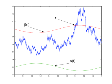
Figure 1: A demonstration of a sample path $X$, and domain $\Gamma$ bounded by lower barrier $\alpha$ and upper barrier $\beta$.

Throughout the paper, $\alpha,\beta\in C[0,1]$ are given satisfying $\alpha(t)<\beta(t)$ for all $t\in[0,1]$. The domain of our interest is defined by all the points bounded by $\alpha$ and $\beta$, that is,

$$\Gamma=\{(a,t):\alpha(t)<a<\beta(t),t\in[0,1]\}.$$

The cross-section $\Gamma(t)=(\alpha(t),\beta(t))\subset\mathbb{R}$ may be time-dependent. We also denote its boundary by

$$\partial\Gamma=\{(\alpha(t),t):t\in[0,1]\}\cup\{(\beta(t),t):t\in[0,1]\}.$$

Consider an $\mathbb{F}$-adapted continuous process $X:[0,1]\times\Omega\mapsto C[0,1]$ with initial $X(0)\in(\alpha(0),\beta(0))$. Let $\tau$ be the first hitting time to the boundary of the time-dependence domain

$$\tau=\inf\{t>0:X(t)\notin\Gamma(t)\}\wedge 1.$$ (1)

Now we introduce the notion of projection operator (see [3]) $\Pi:D[0,1]\times[0,1]^{m}\mapsto\mathbb{R}^{m}$ as

$$\Pi(x,\nu)=(x(\nu_{1}),\ldots,x(\nu_{m}))^{\prime}\quad\forall x\in D[0,1],\nu\in[0,1]^{m}.$$ (2)

For $x\in D[0,1]$, we define a maximum process $x^{*}$ by $x^{*}(t)=\sup_{0\leq s\leq t}x(t)$. It is easy to check that $x^{*}\in D[0,1]$. For some measurable function $g:\mathbb{R}^{4m+1}\to\mathbb{R}$, we are interested in the computation of the objective functional $V:C[0,1]\mapsto\mathbb{R}$ defined by, for given $\{\nu^{(i)}\in\mathbb{[}0,1]^{m}:i=1,2,3,4\}$

$$V=\mathbb{E}[g(\Pi(X,\tau\nu^{(1)}),\Pi(X,\nu^{(2)}),\Pi(X^{*},\tau\nu^{(3)}),\Pi(X^{*},\nu^{(4)}),\tau)].$$ (3)

Note that random times $\tau_{j}=\tau\nu^{(1)}_{j}$ are only measurable with respect to $\mathcal{F}_{1}$, but may not be stopping times whenever $\nu^{(1)}_{j}<1$. Moreover, the value function may be a measurable function depending on the initial states $V(x,t)$ if the functional $V$ is given as a non-path-dependent form of $\mathbb{E}[f(X(T)]$ for some function $f:\mathbb{R}\mapsto\mathbb{R}$. However, we emphasize that our main interest is the computation when the functional is path-dependent in the form of (3), which has a wide range of applications in mathematical finance.

Remark 1

Related literature in connection with a hitting time under a Markovian framework can be found in Dufour and Piunovskiy [6], de Saporta, et al. [5], and Szpruch and Higham [20] among others. In particular, in [6], the existence of optimal stopping with constraints is established using a convex analytic approach. A numerical method for optimal stopping of piecewise deterministic Markov processes is considered in [5]. Bounds for the convergence rate of their algorithms are obtained by introducing quantization of the post jump location and path-adapted time discretization grids. In [20], an application in physics (thermodynamic limit) involving mean hitting time behavior is considered.

1.2 Examples

The evaluation of path-dependent objective functions is of great interest in many networked systems as well as in financial applications such as the option pricing. In particular, the value $V$ of (3) can be considered as a general form of a class of option prices including look-back option, rebate/barrier option, Asian option, Bermuda option etc. To illustrate, consider the underlying stock price $X$ that is a non-negative continuous martingale process under $\mathbb{P}$ that is the corresponding equivalent local martingale measure. Throughout this subsection, we also assume that interest rate is $r\geq 0$, and $\nu^{(i)}=\frac{1}{m}(1,2,\ldots,m)^{\prime}$, $-\alpha(t)=\infty$ and $\beta(t)=1$. Thus, the first hitting time can be written by

$$\tau=\inf\{s>0:X(s)\notin(-\infty,1)\}\wedge 1.$$

We also assume the distribution of $X$ under $\mathbb{P}$ has no atom. In particular, $\mathbb{P}\{X(t)=c\}=0$ for all $c>0$ and $t>0$.

Example 1 (Barrier option)

A barrier option is an option with a payoff depending on whether, within the life of the option, the price of the underlying asset reaches a specified level (the so-called barrier); see more details in [16]. There are three basic types of barrier options: Knock-out options, Knock-in options, and Rebate options. As an illustration, we consider up-and-in barrier call with strike $1/2$ at maturity $T=1$, which is one special case of Knock-in options. Roughly speaking, up-and-in call activates (knocks-in) its payoff $(X(1)-1/2)^{+}$ if the upper barrier is touched before the expiration $T=1$. The precise price formula of the up-and-in call is given by

$$V=e^{-r}\mathbb{E}[(X(1)-\frac{1}{2})^{+}I_{[0,1)}(\tau)]=e^{-r}\mathbb{E}[(X(1)-\frac{1}{2})^{+}I_{[1,\infty)}(X^{*}(1))].$$

In this case, the payoff function is

$$g(x_{1},x_{2},\ldots,x_{4m+1})=e^{-r}(x_{2m}-\frac{1}{2})^{+}I_{[1,\infty)}(x_{4m}),$$

which is discontinuous at $x_{4m}=1$.

Example 2 (Discrete-monitoring-barrier option)

In the related literature, most works assume continuous monitoring of the barrier like Example 1. However, in practice most barrier options traded in markets are monitored at discrete time. Unlike their continuous-time counterparts, there is essentially no closed form solution available, and even numerical pricing is difficult; see more related discussions in[4] and [12]. For instance, the price formula of up-and-in barrier call monitoring at discrete time instants $\{1/m,2/m,\ldots,m-1/m,1\}$ with strike $1/2$ is

$$V=e^{-r}\mathbb{E}\Big{[}\Big{(}X(1)-\frac{1}{2}\Big{)}^{+}I_{[1,\infty)}(\max_{1\leq i\leq m}X(i/m))\Big{]}.$$ (4)

The payoff function $g$ is written as

$$g(x_{1},x_{2},\ldots,x_{4m+1})=e^{-r}(x_{2m}-\frac{1}{2})^{+}I_{[1,\infty)}(\max_{m+1\leq i\leq 2m}x_{i}).$$

Note that $g$ has linear growth, is unbounded, and is discontinuous.

1.3 Computational Methods

To evaluate the path-dependent objective functions, a major difficulty arises from the lack of Markovian property. This rules out the possibility of the conventional numerical-PDE-based methods including the finite difference or finite element methods. In addition, the time-dependent barriers $\alpha$ and $\beta$ also create additional layer of the difficulty. In this paper, we consider Monte Carlo methods to obtain a feasible estimate of the path-dependent problems. Monte Carlo method is a class of computational algorithms that relies on some repeated random sampling to evaluate its deterministic value using its probabilistic fact. This includes Euler-Maruyama approximation [11] and Markov chain approximation [8], [13], and [14] among others.

The general idea of the Monte Carlo method in this vein is the following. For each sample point $\omega\in\Omega$, use $X^{h}(\cdot,\omega)\in D[0,1]$ to denote a simulated path for the underlying process $X(\cdot,\omega)\in C[0,1]$ by a certain Monte Carlo method with a small parameter $h$ (maybe a step size). Define the approximated stopping time by

$$\tau^{h}=\inf\{t>0:X^{h}(t)\notin(\alpha(t),\beta(t))\}\wedge 1.$$

One can approximate $V$ in this way by computing

$$V^{h}=\mathbb{E}[g(\Pi(X^{h},\tau^{h}\nu^{(1)}),\Pi(X^{h},\nu^{(2)}),\Pi(X^{h,*},\tau^{h}\nu^{(3)}),\Pi(X^{h,*},\nu^{(4)}),\tau^{h})].$$ (5)

The main task of this approximating scheme is to design an appropriate Monte Carlo method so that the desired convergence takes place eventually, i.e.,

$$\lim_{h\to 0}V^{h}=V.$$

As the objective value is given as an expectation of (3), $V$ is invariant under the same distribution, and the usual requirements for the Monte Carlo method are intuitively given as follows:

1. $X^{h}$ converges weakly to $X$ as $h\to 0$, denoted by $X^{h}\Rightarrow X$.

2. $g$ is continuous.

A couple of natural questions are as follows.

• Are (H1)-(H2) sufficient to guarantee the desired convergence $\lim_{h\to 0}V^{h}=V$?

• Can (H2) be possibly weakened to some discontinuous function $g$ so that the barrier option pricing (see Section 1.2) can be included?

1.4 Counter Examples

Interestingly, there exist circumstances that lead to counter examples in connection with the desired convergence under (H1)-(H2).

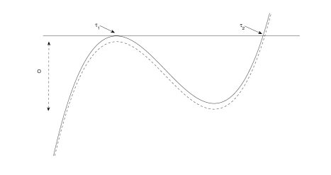
Figure 2: Demonstration of tangency problem: The sample paths of the two processes (solid line and dotted line) are fairly close to each other, but their first exit times are far apart indicating a loss of continuity.

A noticeable counter example is given in Figure 2, which is motivated by the so-called tangency problem. Consider two underlying processes $X^{1}$ (solid line) and $X^{2}$ (dotted line) in Figure 2. No matter how close $X^{1}$ and $X^{2}$ be at the initial states, the difference between their first exit time $\tau_{1}$ and $\tau_{2}$ could be far away; see [2]. The above idea is illustrated in the following example.

Example 3

Let $\{X(s):0\leq s\leq 1\}$ be a deterministic process given by $X(s)=1-(s-\frac{1}{2})^{2}$. Let $\alpha({s})=-\infty$ and $\beta_{s}=1$ for all $s\geq 0$. Then the exit time of $X$ is

$$\tau=\inf\{s>0:X(s)\notin(\alpha({s}),\beta({s}))\}\wedge 1=\frac{1}{2}.$$

Define a family of processes parameterized by $h$ with $X^{h}(s)=X(s)-h$. Although $X^{h}$ converges to $X$ in $L^{\infty}$ as $h\to 0^{+}$, we note that

$$\tau^{h}=\inf\{s>0:X^{h}(s)\notin(\alpha(s),\beta(s))\}\wedge 1=1$$

not converging to $\tau=1/2$.

The next example gives a very different aspect from the first one in the sense that there are no barriers and the underlying process is a Bessel process. This system is often used in finance to model the dynamics of asset prices, of the spot rate and of the stochastic volatility, or as a computational tool. In particular, computations for the celebrated Cox-Ingersoll-Ross (CIR) and Constant Elasticity Variance (CEV) models can be carried out using Bessel processes.

Example 4

Let $X(t)$ be a Bessel process of order $3$ with initial $X(0)=1$, i.e.,

$$X(t)=1+W(t)+\int_{0}^{t}\frac{ds}{X(s)},$$ (6)

which is a well known strict local martingale with $\mathbb{E}[X(1)]<1$; see Page 336 of [9]. A sample path of $X(t)$ is given in Figure 3. Define $X^{h}(t)=X(t)\wedge\frac{1}{h}$. Fix a vector $\nu=(t_{1}\leq\cdots\leq t_{n})^{\prime}\in[0,1]^{n}$, then we have by definition $\Pi(X^{h},\nu)\to\Pi(X,\nu)$ a.s., and the weak convergence $\Pi(X^{h},\nu)\Rightarrow\Pi(X,\nu)$ takes place. Moreover, Kolmogorov consistency theorem together with the uniqueness of the weak solution of SDE (6) implies that $X^{h}\Rightarrow X$ due to the arbitrariness of $n$ and $\nu\in[0,1]^{n}$. However, since $X^{h}$ is a bounded local martingale, it is a martingale. Thus we have $\lim_{h\to 0}\mathbb{E}[X^{h}(1)]=1>\mathbb{E}[X(1)].$

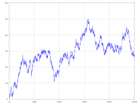
Figure 3: A sample path of Bessel process of order 3

1.5 Goal and Outline of the Paper

The above examples show that (H1)-(H2) may not be sufficient for Monte Carlo simulation to be convergent to the right value of (3). This suggests the following question:

• Given $X^{h}\Rightarrow X$, what are sufficient conditions to ensure the convergence $\lim_{h\to 0}V^{h}=V$? Is it possible to weaken the continuity of $g$ to cover the barrier option?

In this paper, we first present a rigorous proof of the convergence in Section 2. The results in Theorem 5 provide a set of sufficient conditions for the convergence. It can also explain why Examples 3 and 4 do not work.

Our approach is based on the actual computations using Skorohod metric in the space $D[0,1]$. This is the first attempt in this context to the best of our knowledge. Such an approach is advantageous. For example, the study of Monte Carlo convergence usually varies with the particular form of the underlying payoff functions; see [8] and the references therein. However, Theorem 5 provides a unified theoretical basis for the convergence in a general path-dependent form with possibly discontinuous payoff function $g$ and finite time-dependent barrier $(\alpha(t),\beta(t))$. This covers a wider range of applications of Theorem 5 to various types of options, for instance, barrier options, Asian options, look back options, etc. It is also notable that the assumptions on the barrier in the path-dependent problem have some similarities to that imposed for stochastic controlled exit problems; see [2]. To complete the approximation of the value $V$ of (3), one should consider the following question in addition to (Q1).

• Given $X$, how does one construct an approximating sequence of processes $X^{h}$ such that $X^{h}\Rightarrow X$?

Among many of the possible answers to (Q2), we will mainly focus on the construction of $X^{h}$ in the framework of Markov chain approximation in Section 3. Recall that from the book [14], a family of continuous approximating processes $X^{h}$ constructed using Markov chain is convergent to $X$ in distribution if the Markov chain satisfies the local consistency [14, equation (9.4.2)]; see also [14, Theorem 10.4.1]. Compared to [14], we investigate the weak convergence for more generalized local consistency condition. This enables us to cover various types of Monte Carlo simulations in the framework of Markov chain approximation to verify its weak convergence using the generalized local consistency. It essentially extends the use of Markov chain approximation.

To proceed, the rest of the paper is arranged as follows. Section 2 provides sufficient conditions for the convergence of the approximating path-dependent functional $V^{h}$ to the original functional $V$ given that there exists a sequence of random processes $X^{h}$ converging to the original process $X$ weakly. Section 3 addresses the question how to find a sequence of weak convergent $X^{h}$ when the original process $X$ is the solution of a stochastic differential equation. Since Section 3 does not use any result obtained in Section 2, these two sections are independently accessible to the reader. Finally, the paper is concluded with a demonstrating example on discrete-monitoring-barrier options together with some further remarks in Section 4.

2 Sufficient Conditions for Convergence

2.1 Preliminaries

We use the notation given in [3]. Define a metric on $D[0,1]$ by

$$\|x-y\|=\sup_{t\in[0,1]}|x(t)-y(t)|,\ \forall x,y\in D[0,1].$$

Then, the continuous function space on $[0,1]$, denoted by $C[0,1]$, is complete with respect to the uniform topology with the above metric $\|\cdot\|$. On the other hand, the RCLL function space defined on $[0,1]$, denoted by $D[0,1]$, is equipped with the Skorohod topology with the metric

$$\|x-y\|_{s}=\inf_{\lambda\in\Lambda}\{\|\lambda-\mathbb{I}\|,\|x\circ\lambda-y\|\},\ \forall x,y\in D[0,1],$$

where $x\circ y$ denotes the composite function of $x$ and $y$, and $\Lambda$ is the collection of all continuous increasing functions $\lambda$ on $[0,1]$ with $\lambda(0)=0$ and $\lambda(1)=1$, and $\mathbb{I}\in\Lambda$ is identity mapping. It is often useful to use the following fact: $x_{n}\to x$ in Skorohod topology if and only if there exists $\lambda_{n}\in\Lambda$ such that

$$\|\lambda_{n}-\mathbb{I}\|\to 0,\quad\|x_{n}-x\circ\lambda_{n}\|\to 0,\hbox{ as }n\to\infty.$$ (7)

Note that $D[0,1]$ is not complete under the metric $\|\cdot\|_{s}$, but it is complete under an equivalent metric $\|\cdot\|^{o}_{s}$ defined by

$$\|x-y\|_{s}^{o}=\inf_{\lambda\in\Lambda}\Big{\{}\sup_{s<t}\Big{|}\log\frac{\lambda(t)-\lambda(s)}{t-s}\Big{|},\|x-y\|\Big{\}},\ \forall x,y\in D[0,1].$$

For notational convenience, we will use $\|\cdot\|_{s}$ for the metric of $D[0,1]$ in the rest of the paper. In particular, for a mapping $F:D[0,1]\mapsto\mathcal{M}$ with metric space $(\mathcal{M},\|\cdot\|_{\mathcal{M}})$, $F$ is said to be continuous at some $x\in D[0,1]$ if

$$\lim_{n\to\infty}\|F(x_{n})-F(x)\|_{\mathcal{M}}=0\ \hbox{ whenever }\ \lim_{n\to\infty}\|x_{n}-x\|_{s}=0.$$

In contrast, $x\in D[0,1]$ is said to be continuous at some $t\in(0,1)$, if

$$\lim_{n\to\infty}|x(t_{n})-x(t)|=0\ \hbox{ whenever }\ \lim_{n\to\infty}|t_{n}-t|=0.$$

2.2 Some Continuous Mappings Under Skorohod Topology

In this section, we will discuss continuity of some useful mappings on $D[0,1]$ with respect to Skorohod topology. Recall that, for $x\in D[0,1]$, we define $x^{*}\in D[0,1]$ by $x^{*}(t)=\sup_{0\leq s\leq t}x(s)$. We also define a mapping $\mathcal{M}:D[0,1]\mapsto D[0,1]$ as

$$\mathcal{M}(x)=x^{*}.$$

In addition, we are interested in the projection $\Pi$ in (2) given by

$$\Pi(x,\nu)=(x(\nu_{1}),\ldots,x(\nu_{m}))^{\prime}\quad\forall x\in D[0,1],\nu\in[0,1]^{m}$$

and a mapping $\pi:D[0,1]\mapsto[0,1]$ defined by

$$\pi(x)=\inf\{t:x(t)\notin(\alpha(t),\beta(t))\}\wedge 1.$$ (8)

Lemma 2

$\mathcal{M}$ is continuous on $D[0,1]$.

Proof: Since $\lambda$ is strictly increasing, $x^{*}\circ\lambda=(x\circ\lambda)^{*}$. Therefore,

$$\begin{array}[]{ll}\|x^{*}-y^{*}\|_{s}&\displaystyle=\inf_{\lambda\in\Lambda}\{\|\lambda-\mathbb{I}\|,\sup_{t\in[0,1]}|x^{*}(\lambda(t))-y^{*}(t)|\}\\ &\displaystyle=\inf_{\lambda\in\Lambda}\{\|\lambda-\mathbb{I}\|,\sup_{t\in[0,1]}|(x\circ\lambda)^{*}(t)-y^{*}(t)|\}\\ &\displaystyle\leq\inf_{\lambda\in\Lambda}\{\|\lambda-\mathbb{I}\|,\sup_{t\in[0,1]}\sup_{0\leq s\leq t}|(x\circ\lambda)(s)-y(s)|\}\\ &\displaystyle=\inf_{\lambda\in\Lambda}\{\|\lambda-\mathbb{I}\|,\|x\circ\lambda-y\|\}=\|x-y\|_{s}.\end{array}$$

So, ${\mathcal{M}}$ is continuous in ${D[0,1]}$ with respect to the Skorohod topology. $\Box$

Lemma 3

$\Pi$ is continuous at $(x,\nu)\in D[0,1]\times[0,1]^{m}$ whenever $x$ is continuous at each $\nu_{i}$ of $i=1,2,\ldots,m$.

Proof: Given a sequence of vectors $\nu^{(n)}\to\nu$, we observe that

$$|\Pi(x,\nu^{(n)})-\Pi(x,\nu)|\leq\sum_{i=1}^{m}|x(\nu_{i}^{(n)})-x(\nu_{i})|,$$

and the continuity of $\Pi$ in the variable $\nu$ follows directly from the continuity of $x$ at $\nu_{i}$ for each $i$. Next, we show the continuity of $\Pi$ in the variable $x$. To proceed, we fix $\nu$, and an arbitrary sequence $\{x_{n}\}$ satisfying $\lim_{n}\|x_{n}-x\|_{s}=0$. Then, there exists $\{\lambda_{n}\}$ satisfying (7). Therefore, we have

$$\begin{array}[]{ll}|\Pi(x_{n},\nu)-\Pi(x,\nu)|&\displaystyle=\sum_{i=1}^{m}|x_{n}(\nu_{i})-x(\nu_{i})|\\ &\displaystyle\leq\sum_{i=1}^{m}(|x_{n}(\nu_{i})-x(\lambda_{n}(\nu_{i}))|+|x(\lambda_{n}(\nu_{i}))-x(\nu_{i})|)\\ &\displaystyle\leq\|x_{n}-x\circ\lambda_{n})\|+\sum_{i=1}^{m}|x(\lambda_{n}(\nu_{i}))-x(\nu_{i})|\end{array}$$

Note that the first term $\|x_{n}-x\circ\lambda_{n}\|\to 0$ as $n\to\infty$ by (7). On the other hand, since $\|\lambda_{n}-\mathbb{I}\|\to 0$ as $n\to\infty$ by (7), we have $|\lambda_{n}(\nu_{i})-\nu_{i}|\to 0$ as $n\to\infty$. Hence, the second term $\sum_{i=1}^{m}|x(\lambda_{n}(\nu_{i}))-x(\nu_{i})|$ by continuity of $x$ at $\nu_{i}$. Thus, we conclude the continuity of $\Pi$ in the variable $x$. $\Box$

The continuity of $\pi$ of (8) is a rather tricky part. To proceed, let us partition the space $C[0,1]$ as follows: Define

$$C_{1}=\{x\in C[0,1]:\pi(x)<1,\ x(\pi(x))=\beta({\pi(x)}),\ \inf\{t>\pi(x):x(t)>\beta(t)\}=\pi(x)\},$$

$$C_{2}=\{x\in C[0,1]:\pi(x)<1,\ x(\pi(x))=\alpha({\pi(x)}),\ \inf\{t>\pi(x):x(t)<\alpha(t)\}=\pi(x)\},$$

and

$$C_{3}=\{x\in C[0,1]:\pi(x)=1\},\hbox{ and }C_{4}=C[0,1]\setminus(\cup_{i=1}^{3}C_{i}).$$

Accordingly, we can write $C[0,1]=\cup_{i=1}^{4}C_{i}$ and $C_{i}\cap C_{j}=\emptyset$ for $i\neq j$. As for the illustration, one can see that the four curves depicted in Figure 4 belong to four different subsets separately, that is, $L_{i}\in C_{i}$ for $i=1,2,3,4$.

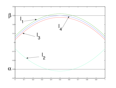
Figure 4: Illustration for the partition of $C[0,1]$

Lemma 4

The $\pi$ defined in (8) is continuous at each $x\in\cup_{i=1}^{3}C_{i}$.

Proof: First, $\pi$ is continuous at $x\in C_{3}$ thanks to Lemma 2. We assume $-\alpha(t)+\beta(t)<\infty$ for each $t$ without loss of generality. Fix $x\in C_{1}$, and $\{x_{n}\}$ be an arbitrary sequence in $D[0,1]$ satisfying $\|x_{n}-x\|_{s}\to 0$ as $n\to\infty$. By the definition of $\|\cdot\|_{s}$, it implies that there exists $\lambda_{n}\in\Lambda$ such that

$$\|\lambda_{n}-\mathbb{I}\|\to 0,\quad\|x_{n}\circ\lambda_{n}-x\|\to 0,\hbox{ as }n\to\infty.$$ (9)

• Case 1. Define, for any $\varepsilon>0$

  $$\delta_{\varepsilon}:=\frac{1}{2}\sup_{\pi(x)<t<\pi(x)+\varepsilon}(x(t)-\beta(t)).$$

  By the definition of $C_{1}$, we have $\delta_{\varepsilon}>0$ for all $\varepsilon>0$. Moreover, by continuity of $x$, there exists a time $t_{\varepsilon}\in(\pi(x),\pi(x)+\varepsilon)$ such that $x(t_{\varepsilon})>\beta(t_{\varepsilon})+\delta_{\varepsilon}$. Next, we observe that

  $$|x_{n}(\lambda_{n}(t_{\varepsilon}))-x(t_{\varepsilon})|\leq\|x_{n}\circ\lambda_{n}-x\|\to 0,\ \hbox{ as }n\to\infty.$$

  This implies that for some large $N_{\varepsilon,1}$

  $$x_{n}(\lambda_{n}(t_{\varepsilon}))\geq x(t_{\varepsilon})-\frac{\delta_{\varepsilon}}{2}>\beta(t_{\varepsilon})+\frac{\delta_{\varepsilon}}{2},\ \forall n\geq N_{\varepsilon,1}.$$ (10)

  On the other hand, there exists $r_{\varepsilon}>0$ due to the continuity of $\beta$ such that

  $$\sup_{t_{\varepsilon}-r_{\varepsilon}<t<t_{\varepsilon}+r_{\varepsilon}}|\beta(t)-\beta(t_{\varepsilon})|<\frac{\delta_{\varepsilon}}{4}.$$

  Moreover, since $\|\lambda_{n}-\mathbb{I}\|\to 0$, we have for some large enough $N_{\varepsilon,2}$,

  $$\|\lambda_{n}-\mathbb{I}\|<r_{\varepsilon},\ \forall n\geq N_{\varepsilon,2}.$$

  Therefore, it leads to

  $$|\beta(\lambda_{n}(t_{\varepsilon}))-\beta(t_{\varepsilon})|\leq\sup_{t_{\varepsilon}-r_{\varepsilon}<t<t_{\varepsilon}+r_{\varepsilon}}|\beta(t)-\beta(t_{\varepsilon})|<\frac{\delta_{\varepsilon}}{4},\ \forall n\geq N_{\varepsilon,2}.$$ (11)

  Inequality (10) together with (11) implies

  $$x_{n}(\lambda_{n}(t_{\varepsilon}))\geq\beta(\lambda_{n}(t_{\varepsilon}))+\frac{\delta_{\varepsilon}}{4},\ \forall n\geq N_{\varepsilon}:=\max\{N_{\varepsilon,1},N_{\varepsilon,2}\},$$

  or equivalently,

  $$\pi(x_{n})\leq\lambda_{n}(t_{\varepsilon})\leq\lambda_{n}(\pi(x)+\varepsilon),\forall n\geq N_{\varepsilon}.$$

  Finally, taking $\lim\sup_{n\to\infty}$ on each side of the above inequality and using $\|\lambda_{n}-\mathbb{I}\|\to 0$ of (9), we have

  $$\lim\sup_{n\to\infty}\pi(x_{n})\leq\lim\sup_{n\to\infty}\lambda_{n}(\pi(x)+\varepsilon)=\pi(x)+\varepsilon.$$

  So we conclude that by the arbitrariness of $\varepsilon$,

  $$\lim\sup_{n\to\infty}\pi(x_{n})\leq\pi(x).$$

• Case 2. We prove the reverse inequality. By the definition of the first hitting time, for any $\varepsilon>0$, there exists $\delta_{\varepsilon}>0$ such that

  $$(\beta-x)^{*}(\pi(x)-\varepsilon)>\delta_{\varepsilon},\ (x-\alpha)^{*}(\pi(x)-\varepsilon)>\delta_{\varepsilon}.$$ (12)

  Also, (9) implies that, $\|\alpha\circ\lambda_{n}-\alpha\|\to 0$, $\|\beta\circ\lambda_{n}-\beta\|\to 0$ and $\|x_{n}\circ\lambda_{n}-x\|\to 0$. Using the triangle inequality, we have

  $$\|(x_{n}-\alpha)\circ\lambda_{n}-(x-\alpha)\|\to 0,\ \|(x_{n}-\beta)\circ\lambda_{n}-(x-\beta)\|\to 0.$$

  So, there exists a large $N_{\varepsilon}$ such that

  $$\|(x_{n}-\alpha)\circ\lambda_{n}-(x-\alpha)\|<\frac{\delta_{\varepsilon}}{2},\ \|(x_{n}-\beta)\circ\lambda_{n}-(x-\beta)\|<\frac{\delta_{\varepsilon}}{2},\ \forall n\geq N_{\varepsilon}.$$

  In particular, this leads to

  $$(\alpha-x_{n})\circ\lambda_{n}(t)<(\alpha-x)(t)+\frac{\delta_{\varepsilon}}{2},\ (x_{n}-\beta)\circ\lambda_{n}(t)<(x-\beta)(t)+\frac{\delta_{\varepsilon}}{2},\ \forall t\in[0,1],\ n\geq N_{\varepsilon}.$$

  By taking $\sup_{[0,\pi(x)-\varepsilon]}$ on both sides of the above inequalities and using (12), we have

  $$(x_{n}-\beta)^{*}\lambda_{n}(\pi(x)-\varepsilon)<(x-\beta)^{*}(\pi(x)-\varepsilon)+\frac{\delta_{\varepsilon}}{2}<-\frac{\delta_{\varepsilon}}{2},\ \forall n\geq N_{\varepsilon},$$

  and

  $$(\alpha-x_{n})^{*}\lambda_{n}(\pi(x)-\varepsilon)<(\alpha-x)^{*}(\pi(x)-\varepsilon)+\frac{\delta_{\varepsilon}}{2}<-\frac{\delta_{\varepsilon}}{2},\ \forall n\geq N_{\varepsilon}.$$

  Thus, we have

  $$\pi(x_{n})\geq\lambda_{n}(\pi(x)-\varepsilon),\ \forall n\geq N_{\varepsilon}.$$

  Taking $\lim\inf_{n}$ and using (9) and the fact of the arbitrariness of $\varepsilon$, we have

  $$\lim\inf_{n}\pi(x_{n})\geq\pi(x).$$

Summarizing the above, we have proved the continuity of $\pi$ at $x\in C_{1}$ with respect to the Skorohod topology, i.e., $\lim_{n\to\infty}\pi(x_{n})=\pi(x)$ whenever $x_{n}\to x\in C_{1}$ with respect to the Skorohod topology. Similar arguments as in Cases 1 and 2 yield that $\pi$ is also continuous at $x\in C_{2}$. $\Box$

2.3 Main Convergence Results

In this section, we utilize the continuity properties under Skorohod topology together with the continuous mapping theorem to obtain the main convergence result. To proceed, we make the following assumptions.

• If $\beta<\infty$, then $\mathbb{P}\{(X-\beta)^{*}(1)\geq 0\}>0$. If $\alpha>-\infty$, then $\mathbb{P}\{(-X+\alpha)^{*}(1)\geq 0\}>0$.

Note that Condition (A1) means that the process hits both barriers $\alpha$ and $\beta$ with positive probability, whenever $-\alpha$ or $\beta$ are bounded above. This is not a restriction; it is only imposed for the technical convenience since one can simply set $\alpha(t)=-\infty$ (resp., $\beta(t)=\infty$) for all $t\in[0,1]$, if $X$ never hits $\alpha$ (resp., $\beta$) almost surely in $\mathbb{P}$. If $-\alpha(t)=\beta(t)=\infty$, then $\tau=1$.

• $X$ satisfies $\inf\{t>\tau:X(t)\notin[\alpha(t),\beta(t)]\}=\tau$ almost surely $\mathbb{P}$.

Condition (A2) requires that the boundary $\partial\Gamma$ is regular with respect to the process $X$. Note that for any small $\varepsilon>0$, $X$ exits from $\bar{\Gamma}$ in the interval $(\tau,\tau+\varepsilon)$ under (A2). Loosely speaking, the condition (A2) means that the process $X(t)$ exits $\bar{\Gamma}$ immediately after it hits the boundary at $\tau$. Note that (A2) also implies that

$$\mathbb{P}\{X\in\cup_{i=1}^{3}C_{i}\}=1\hbox{ or equivalently }\mathbb{P}\{X\in C_{4}\}=0.$$

More discussions are referred to Remark 6.

• $g:\mathbb{R}^{4m+1}\to\mathbb{R}$ is an almost surely continuous function with respect to $\mathbb{P}Z^{-1}$, where $Z:=\Pi(X,\tau\nu^{(1)}),\Pi(X,\nu^{(2)}),\Pi(X^{*},\tau\nu^{(3)}),\Pi(X^{*},\nu^{(4)}),\tau)$. In fact, (A3) is equivalent to the following statement: $g$ is only discontinuous at points in a set $\mathcal{N}$ satisfying $\mathbb{P}\{Z\in\mathcal{N}\}=0$; see also Remark 7.

• One of the following conditions holds:

  1. $g$ is a bounded function;

  2. $g$ is a function with linear growth and $\{X^{h}(t):h>0,t\in[0,1]\}$ is uniformly integrable.

Now, we are ready to answer question (Q1).

Theorem 5

Assume (A1)-(A4). Let $X$ be an ${\cal F}_{t}$-adapted continuous process with initial $X({0})=x$, and $X^{h}$ be a sequence of RCLL processes satisfying $X^{h}\Rightarrow X$ as $h\to 0$. Then, $\lim_{h\to 0}V^{h}=V$.

Proof: We rewrite $V$ and $V^{h}$ by

$$V=\mathbb{E}[G(X)]\hbox{ and }V^{h}=\mathbb{E}[G(X^{h})],$$

where $G:D[0,1]\mapsto\mathbb{R}$ is defined by

$$G(x)=g(\Pi(x,\pi(x)\nu^{(1)}),\Pi(x,\nu^{(2)}),\Pi(\mathcal{M}(x),\pi(x)\nu^{(3)}),\Pi(\mathcal{M}(x),\nu^{(4)}),\pi(x)).$$

Note that (A2) implies that $\mathbb{P}\{X\in\cup_{i=1}^{3}C_{i}\}=1.$ Together with (A3) and Lemma 2, 3, 4, we have continuity of $G$ almost surely $\mathbb{P}X^{-1}$. By the continuous mapping theorem [3, Theorem 2.7], we conclude that

$$G(X^{h})\Rightarrow G(X)\hbox{ as }h\to 0.$$

Together with (A4), it results in $\lim_{h\to 0}V^{h}=V$; see [3, P. 25, 31]. $\Box$

Theorem 5 holds under assumptions of (A1)-(A4). Recall that (A1) is not a restriction. We elaborate on (A2), (A3), and (A4) in what follows.

Remark 6 (Discussions on (A2) and Example 3)

In fact, (A2) is a requirement on the regularity of the boundary $\partial\Gamma$ with respect to the process $X$, and it is referred to as $\tau^{\prime}$-regularity for simplicity; see [19]. Note that since $X$ in Example 3 violates $\tau^{\prime}$-regularity (A2), by observing

$$\inf\{t>\tau:X(t)\notin[\alpha(t),\beta(t)]\}\wedge 1=1>1/2=\tau,$$

it yields the convergence to the wrong value. In other words, (A2) is crucial for the investigation of the convergence.

Remark 7 (Discussions on (A3) and Example 1)

Assumption (A3) is the requirement on the function $g$. First of all, it allows discontinuity of $g$, but it cannot be too much discontinuous in the sense that it is at least required to be almost surely continuous. However, it is already enough to include option pricing for the discontinuous payoff such as the barrier option in Example 1. In fact, $g$ of Example 1 given by

$$g(x_{1},x_{2},\ldots,x_{4m+1})=e^{-r}(x_{2m}-\frac{1}{2})^{+}I_{[1,\infty)}(x_{4m}),$$

is continuous only at $\{x_{4m}=1\}$. Suppose the stock price $X$ follows a geometric Brownian motion, then the probability measure $\mathbb{P}$ satisfies $\mathbb{P}\{X^{*}(1)=1\}=0$, and $g$ is continuous almost surely $PZ^{-1}$.

Remark 8 (Discussions on (A4) and Example 4)

In (A4), another issue yet mentioned is the growth condition of $g$. In particular, if $g$ is of linearly growth function of the underlying price like in the call type option, then one can verify the uniform integrability. We have already seen that, for instance, Example 4 converges to a wrong value, since $\{X(t):t\in(0,1)\}$ is not uniformly integrable while the payoff function $g(x)=x$ is linear growth. Recall the definition of uniform integrability. A set of random variables $\{Y_{\gamma}:\gamma\in\Gamma\}$ is said uniformly integrable, if for any $\varepsilon>0$, there exists a compact set $K$ such that

$$\sup_{\gamma\in\Gamma}\mathbb{E}[Y_{\gamma}I_{\{Y_{\gamma}\notin K\}}]<\varepsilon.$$

Note that to ease the verification of the uniform integrability, one can often use Proposition 10 practically rather than the above definition.

3 Weak Convergence of Markov Chain Approximation

3.1 Markov Chain Approximation

In this section, we establish the weak convergence of Markov chain approximation for multidimensional stochastic differential equations. In what follows, $K$ is a generic constant whose value may change at each line.

1. $b$ and $\sigma$ are Lipschitz in $y$ and Hölder-1/2 continuous in $t$, i.e., with $\phi=b$, $\sigma$,

   $$|\phi(y_{1},t_{1})-\phi(y_{2},t_{2})|\leq K(|y_{1}-y_{2}|+|t_{1}-t_{2}|^{1/2}).$$

Let $Y=\{Y(t):t\in[0,1]\}$ be the unique solution of

$$dY(t)=b(Y(t),t)dt+\sigma(Y(t),t)dW(t);\ Y({0})=y,$$ (13)

where $b:\mathbb{R}^{d+1}\mapsto\mathbb{R}^{d}$, $W$ is a standard $\mathbb{R}^{d_{1}}$ Brownian motion, and $\sigma:\mathbb{R}^{d+1}\mapsto\mathbb{R}^{d\times d_{1}}$. Let $t_{0}^{h}=0\leq t_{1}^{h}\leq\cdots\leq t_{N}^{h}=1$ be a sequence of increasing predictable (i.e., $t_{i}^{h}$ is $\mathcal{F}_{i-1}^{h}$-measurable.) random times with respect to a discrete filtration $\{\mathcal{F}_{i}^{h}:i=0,1,\ldots\}$, and $\{Y_{i}^{h}:i=1,2,\ldots N\}$ be a sequence of $\{\mathcal{F}_{i}^{h}\}$-adapted Markov chain in $\mathbb{R}^{d}$ with transition probability

$$\mathbb{P}\{Y_{i+1}^{h}\in dy|Y_{i}^{h}=x,t_{i}^{h}=t\}=p^{h}(t,x,y).$$

We use $Y^{h}=\{Y^{h}(t):t\in[0,1]\}$ to denote piecewise constant interpolation

$$Y^{h}(t)=\sum_{i=0}^{n-1}Y^{h}_{i}I_{\{t_{i}^{h}\leq t<t_{i+1}^{h}\}}.$$ (14)

For notational simplicity, we set $\Delta t_{n}^{h}=t_{n+1}^{h}-t_{n}^{h}$ and $\Delta Y_{n}^{h}=Y_{n+1}^{h}-Y_{n}^{h}$, $\mathbb{E}_{n}^{h}[\ \cdot\ ]:=\mathbb{E}[\ \cdot\ |\mathcal{F}_{n}^{h}]$, and

$$z^{h}(t):=\max\{n\geq 0:t_{n}^{h}\leq t\},\quad\Delta M_{n}^{h}=\Delta Y_{n}^{h}-\mathbb{E}_{n}^{h}[\Delta Y_{n}^{h}].$$

The interpolation of the Markov chain process $Y^{h}$ is said to be locally consistent, if

1. $\mathbb{E}_{n}^{h}[\Delta Y_{n}^{h}]=\mathbb{E}_{n}^{h}[\Delta t_{n}^{h}]\cdot(b(Y_{n}^{h},t_{n}^{h})+O(h))$,

2. $\hbox{cov}(\Delta Y_{n}^{h}|\mathcal{F}_{n}^{h})=\mathbb{E}_{n}^{h}[\Delta t_{n}^{h}]\cdot((\sigma\sigma^{\prime})(Y_{n}^{h},t_{n}^{h})+O({h}))$, where $O(h)$ is either a $d$-dimensional vector or $d\times d$ dimensional matrix that is ${\mathcal{F}}^{h}_{n}$-measurable with each element being $O(h)$.

To proceed, we also require quasi-uniform step size.

1. The step size $\{\Delta t_{i}^{h}\}$ satisfies $\frac{h}{K}\leq\inf_{i}\Delta t_{i}^{h}\leq\sup_{n}\Delta t_{n}^{h}\leq Kh$.

The (QU) condition yields

$$z^{h}(t)\leq Kt/h,\quad z^{h}(t)\sup_{i}\Delta t_{i}^{h}\leq Kt\ \hbox{ almost surely. }$$ (15)

The main goal of this section is to show that $\{Y^{h}(t):t\in[0,1],h>0\}$ is uniformly integrable and $Y^{h}\Rightarrow Y$ as $h\to 0$. Since the entire proof is rather long, we first provide some useful estimates.

Lemma 9

For the stochastic differential equation (13), assume that (A5) is satisfied, and $Y^{h}$ of (14) is a sequence of random processes satisfying the local consistency conditions $($LC1-LC2$)$ and quasi-uniform step size $($QU$)$. Then, the family of random variables $\{Y^{h}(t):t\in[0,1],h>0\}$ satisfies:

$$\mathbb{E}[|Y^{h}(t)|^{2}]\leq K\hbox{ for all }t\in[0,1],$$ (16)

and

$$\mathbb{E}\Big{[}\sup_{0\leq n\leq z^{h}(t)-1}|\sum_{i=0}^{n}\Delta Y_{i}^{h}|^{2}\Big{]}\leq Kt.$$ (17)

Proof: First, we separate the entire estimation into two parts.

$$\begin{array}[]{ll}\mathbb{E}[\sup_{0\leq n\leq z^{h}(t)-1}|\sum_{i=0}^{n}\Delta Y_{i}^{h}|^{2}]=\mathbb{E}[\sup_{0\leq n\leq z^{h}(t)-1}|\sum_{i=0}^{n}\mathbb{E}_{i}^{h}[\Delta Y_{i}^{h}]+\Delta M_{i}^{h}|^{2}]\\ \quad\quad\leq\displaystyle K\mathbb{E}\Big{[}\sup_{0\leq n\leq z^{h}(t)-1}\Big{|}\sum_{i=0}^{n}\mathbb{E}_{i}^{h}[\Delta Y_{i}^{h}]\Big{|}^{2}\Big{]}+K\mathbb{E}\Big{[}\sup_{0\leq n\leq z^{h}(t)-1}\Big{|}\sum_{i=0}^{n}\Delta M_{i}^{h}\Big{|}^{2}\Big{]}:=K\widetilde{I}_{1}+K\widetilde{I}_{2}.\end{array}$$

Note that $\widetilde{I}_{1}$ has the following upper bound by local consistency,

$$\widetilde{I}_{1}\leq\mathbb{E}\Big{[}z^{h}(t)\sum_{i=0}^{z^{h}(t)-1}\Big{|}\mathbb{E}_{i}^{h}[\Delta Y_{i}^{h}]\Big{|}^{2}\Big{]}\leq K\mathbb{E}\Big{[}z^{h}(t)\sum_{n=0}^{z^{h}(t)-1}(\mathbb{E}_{n}^{h}[\Delta t_{n}^{h}])^{2}\cdot(b^{2}(Y_{n}^{h},t_{n}^{h})+O(h^{2}))\Big{]}.$$

Owing to (QU) condition, we can use the inequality (15) to obtain

$$\begin{array}[]{ll}\widetilde{I}_{1}&\leq Kt\mathbb{E}\Big{[}\sum_{n=0}^{z^{h}(t)-1}\mathbb{E}_{n}^{h}[\Delta t_{n}^{h}]\cdot(b^{2}(Y_{n}^{h},t_{n}^{h})+O(h^{2}))\Big{]}\\ &\leq\displaystyle Kt\mathbb{E}\Big{[}\sum_{n=0}^{[Kt/h]-1}\mathbb{E}_{n}^{h}[\Delta t_{n}^{h}\cdot(b^{2}(Y_{n}^{h},t_{n}^{h})+O(h^{2}))\cdot I_{\{n\leq z^{h}(t)-1\}}]\Big{]}.\end{array}$$

In the last line above, the term $(b^{2}(Y_{n}^{h},t_{n}^{h})+O(h^{2}))\cdot I_{\{n\leq z^{h}(t)-1\}}$ can be included into $\mathbb{E}_{n}^{h}$, since it is $\mathcal{F}_{n}^{h}$-measurable. Now we are ready to use the tower property of conditional expectation and regularity condition (A5) and end up with

$$\widetilde{I}_{1}\leq Kt\mathbb{E}\Big{[}\int_{0}^{t}|Y_{s}|^{2}ds\Big{]}+Kt^{2}h^{2}.$$ (18)

On the other hand,

$$\begin{array}[]{ll}\widetilde{I}_{2}&\displaystyle=\mathbb{E}\Big{[}\sup_{0\leq n\leq z^{h}(t)-1}\Big{|}\sum_{i=0}^{n}\Delta M_{i}^{h}\Big{|}^{2}\Big{]}\\ &\displaystyle\leq K\mathbb{E}\Big{[}\Big{|}\sum_{i=0}^{z^{h}(t)-1}\Delta M_{i}^{h}\Big{|}^{2}\Big{]}\ \hbox{ by Doob's Maximal inequality }\\ &\displaystyle=K\mathbb{E}\Big{[}\sum_{i=0}^{z^{h}(t)-1}|\Delta M_{i}^{h}|^{2}\Big{]}\ \hbox{ since }\ \mathbb{E}[(\Delta M_{i}^{h})^{\prime}(\Delta M_{j}^{h})]=0,\forall i\neq j\\ &\displaystyle\leq K\mathbb{E}\Big{[}\sum_{i=0}^{z^{h}(t)-1}\Delta t_{i}^{h}\hbox{tr}(\sigma\sigma^{\prime})(Y_{i}^{h},t_{i}^{h})\Big{]}+Kht\ \hbox{ by (LC2)}.\end{array}$$

where $\hbox{tr}(A)$ denotes the trace of $A$. Together with (A5), this implies that

$$\widetilde{I}_{2}\leq K\mathbb{E}\Big{[}\int_{0}^{t}|Y_{s}^{h}|^{2}ds\Big{]}+Kht.$$ (19)

Combining (18) and (19), it yields that

$$\mathbb{E}\Big{[}\sup_{0\leq n\leq z^{h}(t)-1}|\sum_{i=0}^{n}\Delta Y_{i}^{h}|^{2}\Big{]}\leq Kth+K\mathbb{E}\Big{[}\int_{0}^{t}|Y^{h}(s)|^{2}ds\Big{]}.$$ (20)

Therefore, we have

$$\begin{array}[]{ll}\mathbb{E}[|Y^{h}(t)|^{2}]&\leq K\mathbb{E}[|y|^{2}+|\sum_{i=0}^{z^{h}(t)-1}\Delta Y^{h}_{i}|^{2}]\leq K+K\mathbb{E}[\int_{0}^{t}|Y^{h}(s)|^{2}ds].\end{array}$$

Gronwall’s inequality then yields the result of (16). Plug in (16) to (20), we conclude (17). $\Box$

To proceed, we also need the following convenient proposition for the uniform integrability, and the reader is referred to [7] for the proof of the proposition.

Proposition 10

A family of real-valued random variable $\{Z_{\theta}:\theta\in\Theta\}$ for some index set $\Theta$ is uniformly integrable if $\sup_{\theta}\mathbb{E}[|Y_{\theta}|^{p}]<\infty$ for some $p>1$.

Theorem 11

Under the same assumptions as that of Lemma 9, the family of random variables $\{Y^{h}(t):t\in[0,1],h>0\}$ is uniformly integrable, and $Y^{h}\Rightarrow Y$ as $h\to 0$.

Proof: we conclude first $\{Y^{h}(t):0\leq t\leq T,h>0\}$ is uniformly integrable by Proposition 10 together with (16). We divide the rest of the proof into several steps.

1. We consider the tightness of $\{\mathbb{P}_{h}=\mathbb{P}(Y^{h})^{-1}:h>0\}$. It is enough to verify conditions imposed on Theorem 13.3.2 and the subsequent corollary given in [3].

   1. By Chebyshev’s inequality and (16)

      $$\begin{array}[]{ll}\displaystyle\lim_{a\to\infty}\lim\sup_{h\to 0}\mathbb{P}\{|Y^{h}(t)|\geq a\}&\displaystyle\leq\lim_{a\to\infty}\lim\sup_{h\to 0}\frac{1}{a^{2}}\mathbb{E}[|Y^{h}(t)|^{2}]=0.\end{array}$$

   2. For the purpose of characterization of tightness for discontinuous functions, we need to introduce some notions of modulus of continuity $\omega(Y^{h},\delta)$ and $\omega^{\prime}(Y^{h},\delta)$ as the following. First, define $\omega(Y^{h},\mathcal{I})=\sup_{r_{1},r_{2}\in\mathcal{I}}|Y^{h}(r_{1})-Y^{h}(r_{2})|$ for any subset $\mathcal{I}\subset[0,1]$. We also use $\mathcal{T}(\delta)$ to denote the collection of all $\delta$-sparse partitions of $[0,1]$. Then, for any $\delta>0$, we can define

      $$\omega(Y^{h},\delta)=\sup_{0\leq t\leq 1-\delta}\omega(Y^{h},[t,t+\delta]),\$$

      and

      $$\omega^{\prime}(Y^{h},\delta)=\inf_{\{t_{i}\}\in\mathcal{T}(\delta)}\max_{i}\omega(Y^{h},[t_{i-1},t_{i})).$$

      For the purpose of tightness of discontinuous functions, we also need to introduce modified version of modulus of continuity. Thanks to (17), we have, for an arbitrary $\varepsilon>0$,

      $$\begin{array}[]{ll}\displaystyle\lim_{\delta\to 0}\lim\sup_{h\to 0}\mathbb{P}\{\omega^{\prime}(Y^{h},\delta)\geq\varepsilon\}\\ \displaystyle\quad\displaystyle\leq\lim_{\delta\to 0}\lim\sup_{h\to 0}\mathbb{P}\{\omega(Y^{h},2\delta)\geq\varepsilon\}\\ \displaystyle\quad\displaystyle\leq\lim_{\delta\to 0}\lim\sup_{h\to 0}\frac{1}{\varepsilon^{2}}\mathbb{E}[\omega^{2}(Y^{h},2\delta)]\\ \quad\displaystyle\leq\displaystyle\lim_{\delta\to 0}\lim\sup_{h\to 0}\frac{1}{\varepsilon^{2}}\mathbb{E}\Big{[}\sup_{z^{h}(t)-1\leq n\leq z^{h}(t+2\delta)-1}|\sum_{i=0}^{n}\Delta Y_{i}^{h}|^{2}\Big{]}\\ \quad\leq\displaystyle\lim_{\delta\to 0}\lim\sup_{h\to 0}\frac{1}{\varepsilon^{2}}K\delta=0.\end{array}$$

   As a result, $\{\mathbb{P}_{h}=\mathbb{P}(Y^{h})^{-1}:h>0\}$ is tight.

2. Since $Y^{h}$ is tight, for an arbitrary infinite sequence, there exists a subsequence that has a weak limit. For notational convenience, we denote this subsequence again by $\{Y^{h}\}$, and its limit by $\bar{Y}$. Due to uniqueness of weak solution, it is enough to show that $\bar{Y}$ is the weak solution of (13). Since $Y^{h}\Rightarrow\bar{Y}$, the uniform integrability and (A5) lead to

   $$\begin{array}[]{ll}&\displaystyle\lim_{h\to 0}\mathbb{E}[Y^{h}(t)]=\mathbb{E}[\bar{Y}(t)],\ \hbox{ and }\\ &\displaystyle\lim_{h\to 0}\mathbb{E}[b(Y^{h}(t),t)]=\mathbb{E}[b(\bar{Y}(t),t)].\end{array}$$

   Therefore, if we set

   $$M(t):=\bar{Y}(t)-\bar{Y}(0)-\int_{0}^{t}b(\bar{Y}(s),s)ds,$$

   we have

   $$\begin{array}[]{ll}\mathbb{E}[M(t)]&=\lim_{h\to 0}\mathbb{E}[Y^{h}(t)-Y^{h}(0)-\int_{0}^{t}b(Y^{h}(s),s)ds]\\ &=\displaystyle\lim_{h\to 0}\mathbb{E}\Big{[}\sum_{i=1}^{z^{h}(t)}((Y_{i}^{h}-Y_{i-1}^{h})-\int_{t_{i-1}^{h}}^{t_{i}^{h}}b(Y_{i-1}^{h},t)dt)\Big{]}-\lim_{h\to 0}\mathbb{E}\Big{[}\int_{t_{z^{h}(t)}^{h}}^{t}b(Y_{z^{h}(t)}^{h},s)ds\Big{]}\end{array}$$ (21)

   Regarding the last term above, by linear growth of $b$

   $$\lim_{h\to 0}\mathbb{E}\Big{[}|\int_{t_{z^{h}(t)}^{h}}^{t}b(Y_{z^{h}(t)}^{h},s)ds|\Big{]}\leq\lim_{h\to 0}\mathbb{E}\Big{[}\int_{t_{z^{h}(t)}^{h}}^{t}K+K|Y_{z^{h}(t)}^{h}|ds\Big{]}\leq K\lim_{h\to 0}\mathbb{E}[\Delta t_{z^{h}(t)}^{h}(1+|Y^{h}(t)|)].$$

   Therefore, by (QU) and (16), we conclude that the second term on (21) satisfies

   $$\lim_{h\to 0}\mathbb{E}\Big{[}\int_{t_{z^{h}(t)}^{h}}^{t}b(Y_{z^{h}(t)}^{h},s)ds\Big{]}=0.$$

   As for the first term of (21), using the Hölder continuity in $t$ and the tower property on local consistency

   $$\begin{array}[]{ll}\displaystyle\lim_{h\to 0}\mathbb{E}\Big{[}\sum_{i=1}^{z^{h}(t)}((Y_{i}^{h}-Y_{i-1}^{h})-\int_{t_{i-1}^{h}}^{t_{i}^{h}}b(Y_{i-1}^{h},t)dt)\Big{]}\\ \quad\displaystyle=\lim_{h\to 0}\mathbb{E}\Big{[}\sum_{i=1}^{z^{h}(t)}((Y_{i}^{h}-Y_{i-1}^{h})-b(Y_{i-1}^{h},t)\Delta t_{i-1}^{h}+O(|\Delta t_{i-1}^{h}|^{3/2}))\Big{]}\\ \quad\displaystyle=\lim_{h\to 0}\mathbb{E}\Big{[}\sum_{i=1}^{z^{h}(t)}(\Delta t_{i-1}^{h}O(h)+O(|\Delta t_{i-1}^{h}|^{3/2}))\Big{]}=0.\end{array}$$

   Therefore, $\mathbb{E}[M(t)]=0$. In fact, one uses exactly the same procedure to show $\mathbb{E}[M(t)|\mathcal{F}_{s}]=M(s)$ for any $0\leq s\leq t$, and it concludes $M(t)$ is a martingale.

   Next, we use $\bar{Y}_{l}$ and $Y^{h}_{l}$ to denote the $l$th component of the vector process $\bar{Y}$ and $Y^{h}$, and use $\langle\bar{Y}_{l},\bar{Y}_{m}\rangle(t)$ to denote the cross-variation of two real processes $Y_{l}$ and $Y_{m}$ up to time $t$. Then,

   $$\begin{array}[]{ll}\displaystyle\mathbb{E}|\langle\bar{Y}_{l},\bar{Y}_{m}\rangle(t)-\int_{0}^{t}(\sigma_{l}\sigma_{m})(\bar{Y}(s),s)ds|\\ \quad\displaystyle=\lim_{h\to 0}\mathbb{E}|\langle Y^{h}_{l},Y^{h}_{m}\rangle(t)-\int_{0}^{t}(\sigma_{l}\sigma_{m})(Y^{h}(s),s)ds|\\ \quad\displaystyle=\lim_{h\to 0}\mathbb{E}|\sum_{i=1}^{n}(Y_{l,i}^{h}-Y_{l,i-1}^{h})(Y_{m,i}^{h}-Y_{m,i-1}^{h})-\int_{0}^{t}(\sigma_{l}\sigma_{m})(Y^{h}(s),s)ds|=0.\end{array}$$

   The last equality can be obtained similar to the above owing to $\mathbb{E}[M(t)]=0$, using the local consistency, and regularity assumption (A5) on $\sigma$. Therefore, the cross-variation $\langle\bar{Y}_{l},\bar{Y}_{m}\rangle(t)=\int_{0}^{t}(\sigma_{l}\sigma_{m})(\bar{Y}(s),s)ds$. This again implies that $M(t)$ is a $d$-dimensional martingale process with its quadratic variation $\langle M\rangle(t)=\int_{0}^{t}(\sigma\sigma^{\prime})(\bar{Y}(s),s)ds$. Applying Levy’s martingale characterization on the time-changed Brownian motion, there exists a $d_{1}$-dimensional Brownian motion $B(t)$ such that $M(t)=\int_{0}^{t}\sigma(\bar{Y}(s),s)dB(s)$. Therefore, $\bar{Y}$ is the weak solution of (13).

Summarizing all the above, it leads to the conclusion. $\Box$

3.2 Examples of Weak Convergence of Markov Chain Approximation

The above construction of Markov chain approximation is based on the local consistency, which is slightly different from the local consistency given by [14, Theorem 10.4.1]. As a result, the convergence result of the Markov chain approximation is generalized in the following sense. $\sigma$ and $b$ may be unbounded but have linear growth. Therefore, the geometric Brownian motion is covered by weak convergence result of Theorem 11 as an important application. In fact, locally consistent MC approximation is flexible for its various choices. For illustrations, we give several simple MC approximations for one dimensional process, which is not included in [14].

Example 5

Euler approximation can be considered as a special case of MC approximations. Let $\{Y_{n}^{h}\}$ be a Markov chain generated by

1. $Y_{0}^{h}=y,t_{0}^{h}=0$.

2. Let the transition probability be $\Delta t_{n}^{h}=h$

   $$Y^{h}_{n+1}=Y_{n}^{h}+b(Y_{n}^{h},nh)h+\sigma(Y_{n}^{h},nh)\sqrt{h}N_{n},$$ (22)

   where $\{N_{n}\}$ is a sequence of i.i.d. standard normal random variables. One can easily verify all local consistency conditions. Then assuming (A5), Theorem 11 implies that the piecewise constant interpolation $Y^{h}$ defined in (14) converges weakly to $Y$, the solution to (13).

Example 6

The following MC approximation can be considered as an extension of binomial approximation of Brownian motion. Let $d=d_{1}=1$. Let $\{Y_{n}^{h}\}$ be a Markov chain generated by

1. $Y_{0}^{h}=y,t_{0}^{h}=0$.

2. Let the transition probability be, with $\Delta t_{n}^{h}=h$

   $$\mathbb{P}\Big{(}Y^{h}_{n+1}=Y_{n}^{h}+b(nh,Y_{n}^{h})h\pm\sigma(nh,Y_{n}^{h})\sqrt{h}\Big{|}Y_{n}^{h}\Big{)}=1/2$$ (23)

The above Markov chain is locally consistent since direct computation leads to

1. $\mathbb{E}[\Delta Y_{n}^{h}|Y_{n}^{h}=y,t_{n}^{h}=t]=\mathbb{E}[\Delta t_{n}^{h}|Y_{n}^{h}=y,t_{n}^{h}=t]\cdot b(y,t)$,

2. ${\rm cov}(\Delta Y_{n}^{h}|Y_{n}^{h}=y,t_{n}^{h}=t)=\mathbb{E}[\Delta t_{n}^{h}|Y_{n}^{h}=y,t_{n}^{h}=t]\cdot\sigma^{2}(y,t)$.

Therefore, assuming (A5), the piecewise constant interpolation $Y^{h}$ of the form (14) is convergent to $Y$ of (13) by Theorem 11.

Example 7

Assume $|\sigma|\wedge|1/\sigma|>\epsilon>0$ in addition to (A5). Then one can use a binomial tree type approximation of the diffusion term $\sigma(Y(t),t)dW(t)$ in (13). Let $d=d_{1}=1$. Let $\{Y_{n}^{h}\}$ be a Markov chain generated by

1. $Y_{0}^{h}=y,t_{0}^{h}=0$.

2. Let $\Delta t_{n}^{h}(Y_{n}^{h},t_{n}^{h})=\frac{h}{\sigma^{2}(Y_{n}^{h},t_{n}^{h})}$, and the transition probability be

   $$\begin{array}[]{l}\mathbb{P}\Big{(}Y^{h}_{n+1}=Y_{n}^{h}+b(Y_{n}^{h},t_{n}^{h})\Delta t_{n}^{h}(Y_{n}^{h},t_{n}^{h})\pm\sqrt{h}\Big{|}(Y_{n}^{h},t_{n}^{h})\Big{)}=1/2.\end{array}$$ (24)

Note that this Markov chain satisfies (QU) as well as local consistency since

1. $\mathbb{E}[\Delta Y_{n}^{h}|Y_{n}^{h}=y,t_{n}^{h}=t]=\mathbb{E}[\Delta t_{n}^{h}|Y_{n}^{h}=y,t_{n}^{h}=t]\cdot b(y,t)$,

2. ${\rm cov}(\Delta Y_{n}^{h}|Y_{n}^{h}=y,t_{n}^{h}=t)=\mathbb{E}[\Delta t_{n}^{h}|Y_{n}^{h}=y,t_{n}^{h}=t]\cdot(\sigma^{2}(y,t)+O(h))$.

Therefore, the piecewise constant interpolation $Y^{h}$ of the form (14) is convergent to $Y$ of (13) by Theorem 11.

3.3 Can We Expect the Strong Convergence?

Can We expect strong convergence? In general, the answer is no. To illustrate, we consider a special case of Euler approximation of Example 5. Let $(\Omega,\mathcal{F},\mathbb{P})$ be a probability space, on which $\mathcal{F}_{t}$ is filtration satisfying usual conditions, and $W_{t}$ of (13) is a standard 1-d Brownian motion. We construct strong approximation of Euler-Maruyama’s method by taking on $N_{n}$ of (22) by

$$N_{n}=\frac{W_{n+1}-W_{n}}{\sqrt{h}}.$$

Under assumption (A5), the SDE (13) has a unique strong solution. Suppose $\hat{Y}^{h}$ is a continuous interpolation of Euler approximation of $Y^{h}$ given by

$$\hat{Y}^{h}(t)=\hat{Y}_{nh}^{h}+b(nh,\hat{Y}_{nh}^{h})(t-nh)+\sigma(nh,\hat{Y}_{nh}^{h})(W(t)-W(nh)),\quad\hbox{ for }t\in[nh,nh+h).$$

Then a classical result (see e.g. [15, Theorem 2.7.3]) shows that

$$\mathbb{E}\Big{[}\sup_{0\leq t\leq T}|Y(t)-\hat{Y}^{h}(t)|\Big{]}\leq Kh^{1/2}.$$

However, the above inequality fails for the piecewise constant interpolation of EM approximation $\{Y^{h}\}$. Otherwise, we have following simple counter example. Consider EM approximation of $W_{t}$ on $[0,1]$ by equal step size $h=1/N$. Then, we have

$$\mathbb{E}\Big{[}\sup_{0\leq t\leq 1}|W(t)-W([Nt]/N)|\Big{]}=\mathbb{E}\Big{[}\sup_{1\leq n\leq N}\sup_{(n-1)/N\leq t<n/N}|W(t)-W(\frac{n-1}{N})|\Big{]}.$$

Note that, $\bar{W}(t)=\sqrt{N}W(t/N)$ is a standard Brownian motion w.r.t. a time-scaled filtration. So one can reduce the above equality as

$$\mathbb{E}\Big{[}\sup_{0\leq t\leq 1}|W(t)-W([Nt]/N)|\Big{]}=\frac{1}{\sqrt{N}}\mathbb{E}\Big{[}\sup_{1\leq n\leq N}\Lambda_{n}\Big{]},$$

where $\{\Lambda_{n}\}$ are i.i.d. random variables defined by

$$\Lambda_{n}=\sup_{n-1\leq t<n}|\bar{W}(t)-\bar{W}(n-1)|.$$

Since, $\Lambda_{n}$’s are unbounded iid random variables, $\mathbb{E}\Big{[}\sup_{1\leq n\leq N}\Lambda_{n}\Big{]}$ goes to infinity as $N\to\infty$. This shows that

$$\mathbb{E}\Big{[}\sup_{0\leq t\leq 1}|W(t)-W([Nt]/N)|\Big{]}>O(N^{-1/2}).$$

In conclusion, one cannot expect more than weak convergence merely under local consistency.

4 Ramification and Further Remarks

4.1 Application to Discrete-Monitoring-Barrier Option Underlying Stochastic Volatility

We begin this section with an application of Theorem 5 to the following stochastic volatility model; see [1]. Let $W$ and $B$ be two standard Brownian motions with correlation $\rho$ in the filtered probability space $(\Omega,\mathcal{F},\mathbb{P},\mathcal{F}_{t})$ . Suppose that the stock price follows

$$dX(t)=X(t)(rdt+\sigma(Y(t))dW(t))$$ (25)

with initial $X(0)=x>0$, and that the volatility follows

$$dY(t)=Y(t)(\mu(t)dt+b(t)dB(t))$$ (26)

with initial $Y(0)=y>0$. We consider a discrete-monitoring-barrier option price

$$V=e^{-r}\mathbb{E}\Big{[}\Big{(}X(1)-\frac{1}{2}\Big{)}^{+}I_{[1,\infty)}(\max_{1\leq i\leq m}X(i/m))\Big{]}.$$

given by (4) of Example 2 by the discrete scheme (5).

$$V^{h}=\mathbb{E}[g(\Pi(X^{h},\tau^{h}\nu^{(1)}),\Pi(X^{h},\nu^{(2)}),\Pi(X^{h,*},\tau^{h}\nu^{(3)}),\Pi(X^{h,*},\nu^{(4)}),\tau^{h})],$$

where $g:\mathbb{R}^{4m+1}\mapsto\mathbb{R}$ is of the form

$$g(x_{1},x_{2},\ldots,x_{4m+1})=e^{-r}(x_{2m}-\frac{1}{2})^{+}I_{[1,\infty)}(\max_{m+1\leq i\leq 2m}x_{i}).$$

One can check that $X$ and $Y$ are unique nonnegative strong solution of SDEs (25) and (26), if $\sigma$ satisfies polynomial growth, and $\mu$ and $b$ are Hölder-1/2 continuous. In addition, we assume

non-degeneracy of $X$, i.e., $\sigma(y)>0$ for all $y>0$.

Note that it is possible to have $\sigma(0)=0$ under the above assumption. In this below, we examine the convergence $\lim_{h}V^{h}=V$ when $X^{h}$ is constructed by the Euler approximation of Example 5.

Note that the regularity condition (A2) is satisfied by [18, Proposition A.1] because $\sigma(\cdot)>0$. On the other hand, the payoff function $g$ is only discontinuous at the points in the set $\{\max_{m+1\leq i\leq 2m}x_{i}=1\}$. Thanks to the fact

$$\mathbb{P}\{\max_{1\leq i\leq m}X(i/m)=1\}=0,$$

it implies that $g$ is almost surely continuous with respect to $\mathbb{P}$. Another thing yet to be verified is the uniform integrability of $\{X^{h}(t):h,t\}$, since $g$ is linear growth. Thanks to Theorem 11 together with (A5), we have $X^{h}\Rightarrow X$ and the desired uniform integrability holds. Therefore, we reach the affirmative answer $\lim_{h}V^{h}=V$.

For the simple demonstration, we present a computational result on the above example with the following data. Let the initial stock price be $X_{0}=0.8$. For simplicity, we assume constant interest rate and volatility $r=.1$ and $\sigma=.3$. Suppose stock is monitored monthly, i.e. $m=12$. If we compute $k=5000$ many sample paths, and each sample path is computed by Euler method with $n=60000$ subintervals, then the computational result shows that the $95\%$ interval is $[0.2310,0.2364]$. The total Matlab running time on Macbook Air is 194 seconds. The Matlab code is also available for download at http://01law.wordpress.com/2013/07/18/code/ .

4.2 Further Remarks

This work has been devoted to analyzing approximation to path-dependent functionals. Using the methods of weak convergence, we have provided a unified approach for proving the convergence of numerical approximation of path-dependent functionals for a wide range of applications.

A possible alternative approach to study the convergence may be to evaluate the approximating problem by perturbing the boundary $(\alpha(t),\beta(t))$ to $(\alpha(t)-h,\beta(t)+h)$. For instance, [17] has studied the property of the value function using the aforementioned perturbation when the value function is non-path dependent and HJB equation is available. It is interesting to check if a similar approach works for the path-dependent case.

This paper focused on diffusion models. For future work, it is worthwhile to examine systems driven by pure jump processes, jump diffusions, and systems with an additional factor process such as nowadays popular regime-switching process. Systems with memory (time delays) form another class of important problems. Much work can also be devoted to numerical solutions of various stochastic differential equations, coordination of multi-agent systems, and many Monte Carlo optimization problems in which one needs to treat path-dependent functionals.

References

- [1] E. Bayraktar, K. Kardaras, and H. Xing. Valuation equations for stochastic volatility models. SIAM Journal on Financial Mathematics, 3:351–373, 2012.
- [2] E. Bayraktar, Q.S. Song, and J. Yang. On the continuity of stochastic control problems on bounded domains. Stochastic Analysis and Applications, 29(1):48–60, 2011.
- [3] P. Billingsley. Convergence of Probability Measures. Wiley Series in Probability and Statistics: Probability and Statistics. John Wiley & Sons Inc., New York, second edition, 1999. A Wiley-Interscience Publication.
- [4] M. Broadie, P. Glasserman, and S. G. Kou. Connecting discrete and continuous path-dependent options. Finance Stoch., 3:55–82, 1999.
- [5] B. de Saporta, F. Dufour, K. Gonzalez, Numerical method for optimal stopping of piecewise deterministic Markov processes. Ann. Appl. Probab., Vol. 20, pp. 1607-1637, (2010).
- [6] F. Dufour and A.B. Piunovskiy, Multiobjective stopping problem for discrete-time Markov processes: convex analytic approach, J. Appl. Probab., Vol. 47, pp. 947-966, (2010).
- [7] R. Durrett. Probability. The Wadsworth & Brooks/Cole Statistics/Probability Series. Wadsworth & Brooks/Cole Advanced Books & Software, Pacific Grove, CA, 3rd edition, 2005. Theory and examples.
- [8] P. Glasserman. Monte Carlo Methods In Financial Engineering. Springer, 2004.
- [9] M. Jeanblanc, M. Yor, and M. Chesney. Mathematical Methods for Financial Markets. Springer Finance. Springer-Verlag London Ltd., London, 2009.
- [10] I. Karatzas and S.E. Shreve. Brownian Motion and Stochastic Calculus, Graduate Texts in Mathematics, volume 113. Springer-Verlag, New York, second edition, 1991.
- [11] P.E. Kloeden and E. Platen. Numerical Solution of Stochastic Differential Equations, volume 23 of Applications of Mathematics (New York). Springer-Verlag, Berlin, 1992.
- [12] S. G. Kou. On pricing of discrete barrier options. Statistica Sinica, 13:955–964, 2003.
- [13] H.J. Kushner. Numerical methods for stochastic control problems in continuous time. SIAM J. Control Optim., 28(5):999–1048, 1990.
- [14] H.J. Kushner and P. Dupuis. Numerical Methods for Stochastic Control Problems in Continuous Time, volume 24 of Applications of Mathematics (New York). Springer-Verlag, New York, second edition, 2001.
- [15] X.R. Mao. Stochastic Differential Equations and Applications. Horwood Pub Ltd, 2007.
- [16] R. L. McDonald. Derivatives Markets. Pearson Education, Inc., second edition, 2006.
- [17] Q.S. Song, and G. Yin. Rates of convergence of numerical methods for controlled regime-switching diffusions with stopping times in the costs. SIAM Journal on Control and Optimization, 48(3): 1831–1857, 2009.
- [18] Q.S. Song, G. Yin, and C. Zhu. Optimal switching with constraints and utility maximization of an indivisible market. SIAM Journal on Control and Optimization, 50(2):629–651, 2012.
- [19] D. Stroock and S.R.S. Varadhan. On degenerate elliptic-parabolic operators of second order and their associated diffusions. Comm. Pure Appl. Math., 25:651–713, 1972.
- [20] L. Szpruch and D.J. Higham, Comparing hitting time behavior of Markov jump processes and their diffusion approximations, SIAM Multiscale Model. Simul., Vol. 8, pp. 605–621, (2010).