Dynamic Hubbard model: kinetic energy driven charge expulsion, charge inhomogeneity, hole superconductivity, and Meissner effect

Abstract

Conventional Hubbard models do not take into account the fact that the wavefunction of an electron in an atomic orbital expands when a second electron occupies the orbital. Dynamic Hubbard models have been proposed to describe this physics. These models reflect the fact that electronic materials are generically $not$ electron-hole symmetric, and they give rise to superconductivity driven by lowering of kinetic energy when the electronic energy band is almost full, with higher transition temperatures resulting when the ions are negatively charged. We show that the charge distribution in dynamic Hubbard models can be highly inhomogeneous in the presence of disorder, and that a finite system will expel negative charge from the interior to the surface, and that these tendencies are largest in the parameter regime where the models give rise to highest superconducting transition temperatures. High $T_{c}$ cuprate materials exhibit charge inhomogeneity and they exhibit tunneling asymmetry, a larger tendency to emit electrons rather than holes in NIS tunnel junctions. We propose that these properties, as well as their high $T_{c}$’s, are evidence that they are governed by the physics described by dynamic Hubbard models. Below the superconducting transition temperature the models considered here describe a negatively charged superfluid and positively charged quasiparticles, unlike the situation in conventional BCS superconductors where quasiparticles are charge neutral on average. We examine the temperature dependence of the superfluid and quasiparticle charges and conclude that spontaneous electric fields should be observable in the interior and in the vicinity of superconducting materials described by these models at sufficiently low temperatures. We furthermore suggest that the dynamics of the negatively charged superfluid and positively charged quasiparticles in dynamic Hubbard models can provide an explanation for the Meissner effect observed in high $T_{c}$ and low $T_{c}$ superconducting materials.

I Introduction

The wavefunction of electrons in an atom is self-consistently determined by all the electrons in the atomorbx . The conventional single band Hubbard Hamiltonianhub ; hub2

$$H=-\sum_{i,j,\sigma}[t_{ij}c_{i\sigma}^{\dagger}c_{j\sigma}+h.c.]+U\sum_{i}n_{i\uparrow}n_{i\downarrow}$$ (1)

does not take this well-known fact into account: the atom with two electrons is assumed to change its energy due to electron-electron repulsion, but the electronic wavefunction is assumed to be simply the product of single-electron wavefunctions. This is incorrect because the spacing of electronic energy levels in an atom is always smaller than the electron-electron repulsioninapp . To correct this deficiency we have proposed a variety of new Hamiltoniansholeelec , generically called ‘dynamic Hubbard models’, that take into account the fact that orbital expansion takes place when a non-degenerate atomic orbital is doubly occupied. These Hamiltonians involve either an auxiliary spinhole1 ; tang or boson degree of freedomdynhub , or a second electronic orbitalhole2 .

A simple way to incorporate this physics is by the site Hamiltonianpincus ; dynhub

$$H_{i}=\frac{p_{i}^{2}}{2m}+\frac{1}{2}Kq_{i}^{2}+(U+\alpha q_{i})n_{i\uparrow}n_{i\downarrow}$$ (2)

where $\alpha$ is a coupling constant (assumed positive) and $q_{i}$ a local boson degree of freedom describing the orbital relaxation, with equilibrium position at $q_{i}=0$ if zero or one electrons are present. The Coulomb repulsion between electrons is $U$ when $q_{i}=0$. However, upon double occupancy of the orbital at site $i$, $q_{i}$ will take the value $q_{i}=-\alpha/K$ and the on-site repulsion will be reduced from $U$ to $U_{eff}=U-\alpha^{2}/(2K)$ to give rise to minimum energy, as can be seen from completing the square:

$$H_{i}=\frac{p_{i}^{2}}{2m}+\frac{1}{2}K(q_{i}+\frac{\alpha}{K}n_{i\uparrow}n_{i\downarrow})^{2}+(U-\frac{\alpha^{2}}{2K})n_{i\uparrow}n_{i\downarrow}.$$ (3)

This is a way to describe the orbital relaxationrelax that takes place when the orbital becomes doubly occupied. The conventional Hubbard model corresponds to the limit of an infinitely stiff orbital ($K\rightarrow\infty$) where the orbital does not relax and the on-site $U$ is not reduced.

The importance of this physics increases when the ionic charge (positive) is smalldynhub , since in that case the orbital expansion is larger (for example, the orbital expansion is larger for $H^{-}$ than for $He$), which corresponds to a smaller stiffness parameter $K$ in Eq. (3). The importance of this physics for a lattice system of such atoms also increases as the filling of the electronic energy band increases and there is an increasing number of atoms with doubly occupied orbitals. For these two reasons, the importance of this physics increases the more negative charge the system has. Thus it is reasonable to expect that a lattice system described by this model will have a strong tendency to expel negative chargechargeexp0 ; chargeexp .

Figure 1 depicts the essential physics of dynamic Hubbard models as opposed to conventional Hubbard models: the doubly occupied orbital is larger than the singly occupied orbital. Note also that when an atomic orbital expands, the electronic kinetic energy is lowered, since in an orbital of radial extent $r$ the electron kinetic energy is of order $\hbar^{2}/(2m_{e}r^{2})$, with $m_{e}$ the electron mass. Thus, one can say that in the atom as described by a dynamic Hubbard model there is negative charge expulsion driven by kinetic energy lowering. This is not the case for an atom described by the conventional Hubbard model.

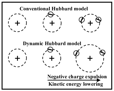
Figure 1: In the conventional Hubbard model the atomic orbital is not modified by electronic occupancy. In the dynamic Hubbard model and in real atoms, addition of the second electron causes orbital expansion due to the electron-electron interaction. Negative charge is expelled outward and the kinetic energy of the electrons is lowered relative to that with a non-expanded orbital.

Just like for the atom, we find for the system as a whole described by a dynamic Hubbard model that there is negative charge expulsion and it is associated with lowering of kinetic energy. Figure 2 shows results of exact diagonalization for a finite lattice that indicate that the electron concentration is considerably larger near the surface than in the interior. We discuss the origin of this effect and the details of the calculation leading to the results shown in Fig. 2 in the following sections.

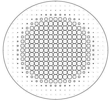
Figure 2: Cylindrical superconductor described by the dynamic Hubbard model. The circles at each lattice site have radius proportional to the hole occupation at the site. Note that the hole occupation is larger in the interior than near the surface, implying that the negative charge concentration is higher near the surface than in the interior.

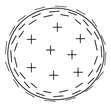
Figure 3: Expected charge distribution in the ground state of superconductors according to the theory of hole superconductivitychargeexp . The superconducting condensation energy and associated charge expulsion originate in lowering of kinetic energy.

The theory of hole superconductivitywebsite ; sns starts from a dynamic Hubbard model and predicts within BCS theorydeltat a superconducting state with some essential differences from the conventional superconducting state. The superconducting condensation energy originates in lowering of $kinetic$ rather than potential energyapparent ; 99 ; prb2000 , and the gap function is energy-dependent with a slope of universal signdeltat . Also, superconductors are predicted to have a non-homogeneous charge distribution in the ground statechargeexp0 , as shown schematically in Fig. 3: excess positive charge in the interior and excess negative charge near the surface, resembling a “giant atom”giantatom . This charge distribution is predicted from modified London-like electrodynamic equationschargeexp , as well as from the energy dependence of the gap functionchargeexp0 . The charge distribution in Fig. 3 is $qualitatively$ similar to that in Figs. 2 and 1.

The finite gap slope of the superconducting gap function predicted by dynamic Hubbard modelsdeltat leads to the prediction of asymmetric tunneling characteristics in NIS tunnel junctionstunasym , with larger current for a negatively biased superconductor, reflecting the tendency of the superconductor to expel electrons. Such asymmetric behavior of NIS tunnel junctions is commonly found in high temperature superconductors.

As a consequence of the charge expulsion physics the superconducting state in systems described by dynamic Hubbard models has quasiparticles that are $positively$ charged on averagethermo , and the superfluid has excess $negative$ charge, in contrast to conventional BCS-London superconductors where quasiparticles are charge neutral on average. We will examine the consequences of this physics for superconductors described by these models at temperatures well below the superconducting transition temperature.

Dynamic Hubbard models are by nature electron-hole $asymmetric$ and so are superconductors, as evidenced by the fact that a rotating superconductor develops a magnetic field that is always parallel, never antiparallel, to the direction of the mechanical angular momentum of the bodyehasym . This suggests that dynamic Hubbard models are more appropriate to describe superconductors than the conventional Hubbard model that is electron-hole symmetric. Furthermore, in dynamic Hubbard models kinetic energy lowering plays a key role, in contrast to conventional Hubbard models. It was pointed out early on by Fritz London thatlondonkinetic “the superfluid state of helium as well as the superconducting state of electrons are fluid” (rather than solid), and that this may arise because “it will be more favorable to give preference to minimizing the kinetic energy”. In his bookslondonbooks , London emphasized this physics for superfluid ${}^{4}He$ but not for superconductors. We have recently pointed out the close relationship between the physics of superconductors as described by the theory of hole superconductivity and superfluid ${}^{4}He$super2 .

A non-uniform charge distribution in a solid gives rise to electrostatic fields and an associated potential energy cost. It will be favored if this cost is compensated by a kinetic energy gain, i.e. lowering of kinetic energy. Thus it is natural to expect that dynamic Hubbard models are prone to develop charge inhomogeneity, and in extreme cases phase separationprb , where the kinetic energy lowering overcompensates for the potential energy cost. High $T_{c}$ cuprates exhibit charge inhomogeneitybianconi ; stripes ; patches ; patches2 , suggesting that dynamic Hubbard models may be useful to describe them.

In superconductors described by the conventional BCS-London theory, no negative charge expulsion occurs, the kinetic energy is raised rather than lowered in the transition to superconductivity, quasiparticles are charge neutral on average, and the Meissner effect is argued to be completely understood within the framework of the conventional theorym1 ; m2 ; m3 ; m4 ; m5 ; m6 ; m7 ; m8 ; m9 ; m10 ; m11 . However, we have argued elsewhere that the conventional theory does not provide a $dynamical$ understanding of the Meissner effectlorentz ; validity . Instead, the negative charge expulsion physics driven by kinetic energy lowering of dynamic Hubbard models discussed here offers a natural explanation for the Meissner effectemf ; meissner : just as in classical plasmas obeying Alfven’s theoremplasma , the magnetic field lines move with the expelled negative charge. The physics of dynamic Hubbard models is proposed to apply to all superconducting materials, in contrast to the conventional theory that is proposed to apply only to “conventional” superconductorscohen ; norman . Given that $all$ superconductors exhibit a Meissner effect, it is useful to remember Isaac Newton’s rule of natural philosophynewton : to the same natural effects we must, as far as possible, assign the same causes.”

II dynamic Hubbard models

We can describe the physics of interest by a multi-orbital tight binding model (at least two orbitals per site)hole2 ; multi2 , or with a background spinhole1 ; color or harmonic oscillatorphonon1 ; phonon2 degree of freedom that is coupled to the electronic double occupancy, as in Eq. (2). Assuming the latter, the site Hamiltonian is given by Eq. (2), and the Hamiltonian can be written as

$$H = -\sum_{i,j,\sigma}[t_{ij}c_{i\sigma}^{\dagger}c_{j\sigma}+h.c.]+\sum_{i}\hbar\omega_{0}a_{i}^{\dagger}a_{i}$$ (4)

$$+ \sum_{i}[U+g\hbar\omega_{0})(a_{i}^{\dagger}+a_{i})]n_{i\uparrow}n_{i\downarrow}$$

with frequency $\omega_{0}=\sqrt{K/m}$ and $g=\alpha/(2K\hbar\omega_{0})^{1/2}$ the dimensionless coupling constant. Estimates for the values of these parameters were discussed in ref. dynhub . Using a generalized Lang-Firsov transformationmahan ; dynhub ; phonon2 ; hawai the electron creation operator $c_{i\sigma}^{\dagger}$ is written in terms of new quasiparticle operators $\tilde{c}_{i\sigma}^{\dagger}$ as

$$c_{i\sigma}^{\dagger} = e^{g(a_{i}^{\dagger}-a_{i})\tilde{n}_{i,-\sigma}}\tilde{c}_{i\sigma}^{\dagger}=[1+(e^{-g^{2}/2}-1)\tilde{n}_{i,-\sigma}]\tilde{c}_{i\sigma}^{\dagger}$$ (5)

$$+ \tilde{n}_{i,-\sigma}\times(incoherent\;part)$$

where the incoherent part describes the processes where the boson goes into an excited state when the electron is created at the site. For large $\omega_{0}$ those terms become small and we will ignore them in what follows, which amounts to keeping only ground state to ground state transitions of the boson field. The electron creation operator is then given by

$$c_{i\sigma}^{\dagger}=[1+(S-1)\tilde{n}_{i,-\sigma}]\tilde{c}_{i\sigma}^{\dagger}$$ (6a)

$$S=e^{-g^{2}/2}$$ (6b)

and the quasiparticle weight for electronic band filling $$n n$$ ( electrons per site) is

$$z(n)=(1+(S-1)\frac{n}{2})^{2}$$ (6c)

so that it decreases monotonically from $1$ when the band is almost empty to $S^{2}<1$ when the band is almost full. The single particle Green’s function and associated spectral function is renormalized by the multiplicative factors on the quasiparticle operators given in Eq. (6a))phonon2 ; undr , which on the average amounts to multiplication of the spectral function by the quasiparticle weight Eq. (6c). This will cause a reduction in the photoemission spectral weight at low energies from what would naively follow from the low energy effective Hamiltonian, an effect extensively discussed in Ref. undr . A corresponding reduction occurs in the two-particle Green’s function and associated low frequency optical propertiesundr ; dynhub12 .

The low energy effective Hamiltonian is then

$$H=-\sum_{ij\sigma}t_{ij}^{\sigma}[\tilde{c}_{i\sigma}^{\dagger}\tilde{c}_{j\sigma}+h.c.]+U_{eff}\sum_{i}\tilde{n}_{i\uparrow}\tilde{n}_{i\downarrow}$$ (7a)

$$t_{ij}^{\sigma}=[1+(S-1)\tilde{n}_{i,-\sigma}][1+(S-1)\tilde{n}_{j,-\sigma}]t_{ij}$$ (7b)

and $U_{eff}=U-\hbar\omega_{0}g^{2}$. Thus, the hopping amplitude for an electron between sites $i$ and $j$ is given by $t_{ij}$, $St_{ij}$ and $S^{2}t_{ij}$ depending on whether there are $0$, $1$ or $2$ other electrons of opposite spin at the two sites involved in the hopping process.

The physics of these models is determined by the magnitude of the parameter $S$, which can be understood as the overlap matrix element between the expanded and unexpanded orbital in Fig. 1. It depends crucially on the net ionic charge $Z$, defined as the ionic charge when the orbital in question is unoccupieddynhub . In Fig. 1, $Z=1$ if the states depicted correspond to the hydrogen ions $H^{+}$, $H$ and $H^{-}$ and $Z=2$ if they correspond to $He^{++}$, $He^{+}$ and $He$. In a lattice of $O^{=}$ anions, as in the $Cu-O$ planes of high $T_{c}$ cuprates, the states under consideration are $O$, $O^{-}$ and $O^{=}$ and $Z=0$, and in the $B^{-}$ planes of $MgB_{2}$, $Z=1$. The effects under consideration here become larger when $S$ is small, hence when $Z$ is small. An approximate calculation of $S$ as a function of $Z$ is given in dynhub .

We now perform a particle-hole transformation since we will be interested in the regime of low hole concentration. The hole creation operator is given by, instead of Eq. (6a)

$$c_{i\sigma}^{\dagger}=[S+(1-S)\tilde{n}_{i,-\sigma}]\tilde{c}_{i\sigma}^{\dagger}$$ (8a)

where $$\tilde{n}_{i,\sigma} n$$ is now the hole site occupation, and the hole quasiparticle weight increases with hole occupation as

$$z_{h}(n)=S^{2}(1+(\frac{1}{S}-1)\frac{n}{2})^{2}$$ (8b)

For simplicity of notation we denote the hole creation operators again by $c_{i\sigma}^{\dagger}$, the hole site occupation by $n_{i\sigma}$ and the effective on-site repulsion between holes of opposite spin $U_{eff}$ (the same as between electrons) by $U$ to simplify the notation. The Hamiltonian for holes is then

$$H=-\sum_{ij\sigma}t_{ij}^{\sigma}[{c}_{i\sigma}^{\dagger}{c}_{j\sigma}+h.c.]+U\sum_{i}{n}_{i\uparrow}{n}_{i\downarrow}$$ (9a)

$$t_{ij}^{\sigma}=t_{ij}^{h}[1+(\frac{1}{S}-1))n_{i,-\sigma}][1+(\frac{1}{S}-1){n}_{j,-\sigma}]$$ (9b)

with $t_{ij}^{h}=S^{2}t_{ij}$ the hopping amplitude for a single hole when there are no other holes in the two sites involved in the hopping process. The hole hopping amplitude and the effective bandwidth increase as the hole occupation increases, and so does the quasiparticle (quasihole) weight Eq. (8b).

Finally, we will assume there is only nearest neighbor hopping $t_{ij}=t$ for simplicity and write the nearest neighbor hopping amplitude resulting from Eq. (9b) as

$$t_{ij}^{\sigma}=t_{h}+\Delta t(n_{i,-\sigma}+n_{j,-\sigma})+\Delta t_{2}n_{i,-\sigma}n_{j,-\sigma}$$ (10a)

with

$$t_{h}=tS^{2}$$ (10b)

$$\Delta t=tS(1-S)$$ (10c)

$$\Delta t_{2}=t(1-S)^{2}=(\Delta t)^{2}/t_{h}.$$ (10d)

The non-linear term with coefficient $\Delta t_{2}$ is expected to have a small effect when the band is close to full (with electrons) and is often neglected. Without that term, the model is also called the generalized Hubbard model or Hubbard model with correlated hoppingkiv ; camp . The effective hopping amplitude for average site occupation $n$ is, from Eq. (10a)

$$t(n)=t_{h}+n\Delta t+\frac{n^{2}}{4}\Delta t_{2}$$ (11)

so that a key consequence of integrating out the higher energy degrees of freedom is to renormalize the hopping amplitude and hence the bandwidth and the effective mass (inverse of hopping amplitude).

Generalized dynamic Hubbard models which include also coupling of the boson degree of freedom to the single site occupation have qualitatively similar physics, since the low energy effective Hamiltonian is also given by Eq. (7). They are discussed in Ref. undr .

III hole pairing and superconductivity in dynamic Hubbard models

As wedeltat and othersoth ; oth2 ; oth3 ; oth4 have discussed, the correlated hopping $\Delta t$ gives a strong tendency to pairing and superconductivity when a band is almost full. The hopping amplitude for a single hole is $t_{h}$, and it increases to $t_{h}+\Delta t$ when the hole hops to or from a site occupied by another hole (of opposite spin), thus giving an incentive for holes to pair to lower their kinetic energy. The superconductivity described by this model has a number of interesting featuresdeltat that we have proposed are relevant to the description of high $T_{c}$ cuprates, namely strong dependence of $T_{c}$ on hole concentrationdeltat , energy dependent gap function and resulting tunneling asymmetry of universal signtunasym , superconductivity driven by kinetic energy lowering and associated low energy optical sum rule violationapparent , change in optical spectral weight at frequencies much higher than the superconducting energy gap upon onset of superconductivitycolor , strong positive pressure dependence of $T_{c}$deltat , increased quasiparticle weight upon entering the superconducting stateundr , etc. Many of these predictions are supported by observations on high $T_{c}$ cuprates made both before and after the predictions were made.

The more fundamental dynamic Hubbard model from which the $\Delta t$ interaction derives has also been studied using Eliashberg theorydynfrank and exact numerical methodsdynhub12 and shows an even stronger tendency to pairing and superconductivity.

IV negative charge expulsion in the normal state of dynamic Hubbard models

We consider the Hamiltonian for holes Eq. (9), with the hopping amplitudes given by Eq. (10). We assume a cylindrical geometry of radius R and infinite length in the z direction. We decouple the interaction terms within a simple mean field approximation assuming $<n_{i\sigma}>=n_{i}/2$ with $n_{i}$ the hole occupation at site $i$, and obtain the mean field Hamiltonian

$$H_{mf}=H_{mf,kin}+H_{mf,pot}$$ (12a)

$$H_{mf,kin}=-\sum_{<ij>,\sigma}[t_{h}+\Delta tn_{i}+\Delta t_{2}\frac{n_{i}^{2}}{4}][c_{i\sigma}^{\dagger}c_{j\sigma}+h.c.]$$ (12b)

$$H_{mf,pot}=\frac{U}{4}\sum_{i}n_{i}^{2}$$ (12c)

Assuming a band filling of $n$ holes per site, we diagonalize the Hamiltonian Eq. (12) with initial values $n_{i}=n$ and fill the lowest energy levels until the occupation $n$ is achieved. From the Slater determinant of that state we obtain new values of $n_{i}$ for each site, and iterate this procedure until self-consistently is achieved. We can extend this procedure to finite temperatures, iterating to self-consistency for a given chemical potential $\mu$. We consider then the resulting occupation of the sites as function of the distance $r$ to the center of the cylinder. Sometimes there are non-equivalent sites at the same distance from the axis (e.g. (5,0) and (3,4)) that yield somewhat different occupation, for those cases we show the average and standard deviation as error bars in the graphs.

Figure 4 shows a typical example of the behavior found. Here we assumed $\Delta t_{2}=0$, corresponding to the simpler Hubbard model with correlated hopping and no six-fermion operator term. Even for $\Delta t=0$ the hole occupation is somewhat larger in the interior than near the surface. When the interaction $\Delta t$ is turned on, the hole occupation increases in the interior and decreases near the surface. This indicates that the system expels electrons from the interior to the surface. Clearly, this occurs because the sites near the surface have lower coordination than those in the interior and thus benefit less from the lowering of kinetic energy associated with higher hole concentration (described by Eq. (12b) than the sites in the bulk. The effect becomes more pronounced when $\Delta t$ is increased, as one would expect.

Figure 5 shows the hole site occupations as circles of diameter proportional to it, for the cases $\Delta t=0$ and $\Delta t=0.25$ of Fig. 4. Note that the interior hole occupation is larger for $\Delta t=0.25$ than it is for $\Delta t=0$, while near the surface the hole occupation is larger for $\Delta t=0$. Again this shows that the system with $\Delta t=0.25$ is expelling electrons from the interior to the surface, thus depleting the hole occupation near the surface.

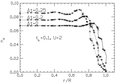
Figure 4: Hole site occupation per spin for a cylinder of radius $R=11$ as function of $r/R$, with $r$ the distance to the center, for a cubic lattice of side length $1$ in the normal state. There are $377$ sites in a cross-sectional area ($\pi R^{2}=380.1$). The average occupation (both spins) is $n=0.126$ holes per site and the temperature is $k_{B}T=0.02$.

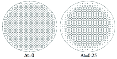
Figure 5: The diameters of the circles are proportional to the hole occupation of the site. Note that for finite $\Delta t$ the hole occupation increases in the interior and is depleted near the surface. The parameters correspond to the cases shown in Fig. 4.

These results are obtained by iteration. Fig. 6 shows the behavior of the energies as a function of iteration number for the cases $\Delta t=0$ and $\Delta t=0.25$ of Fig. 4. The initial values correspond to a uniform hole distribution with each site having the average occupation. The evolution is non-monotonic because in the intermediate steps the overall hole concentration increases, nevertheless it can be seen that for the case $\Delta t=0.25$ the final kinetic energy when self-consistency is achieved is lower, and the final potential energy is higher, associated with the larger hole concentration in the interior and the lower hole concentration near the surface shown in Fig. 4. This is of course what is expected. For the case $\Delta t=0$ instead there is essentially no difference in the energies between the initial uniform state and the final self-consistent state.

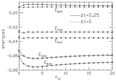
Figure 6: Kinetic, potential and total energy per site for $\Delta t=0.25$ as function of number of iterations starting with a uniform hole distribution.

As the correlated hopping amplitude $\Delta t$ increases, and even more so in the presence of $\Delta t_{2}$, the system appears to develop a tendency to phase separation, where holes condense in the interior and the outer region of the cylinder becomes essentially empty of holes. This happens very rapidly as function of the parameters for the finite system under consideration. Examples are shown in Fig. 7. An analytic derivation of the condition on the parameters in the Hamiltonian and band filling where this occurs is given in ref. prb .

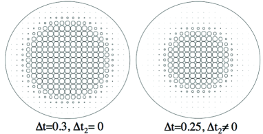
Figure 7: As the correlated hopping terms increase, the system develops a tendency to phase separation, where essentially all the holes condense to the interior. Parameters are the same as in Fig. 4 except as indicated. The maximum hole occupation per spin is 0.128 and 0.214 for the left and right panel, the average hole occupation per spin is 0.063.

In summary, we have seen that the dynamic Hubbard model promotes expulsion of negative charge from the interior to the surface of the system in the normal state when the band is almost full, and that the charge expulsion physics is associated with kinetic energy lowering, just as in the single atom, Fig. 1. When the concentration of holes increases, in other words when the band has fewer electrons, the negative charge expulsion tendency rapidly decreasesprb . The charge expulsion tendency is largest when the parameter $\Delta t$ is largest, which in turn corresponds to smaller $S$, the overlap of the atomic orbitals when one and two electrons are at the orbital. As discussed earlier, $S$ is smaller when the ionic charge $Z$ is smaller, corresponding to a more negatively charged ion. The fact that the effective Hamiltonian derived from this physics expels more negative charge the more negatively charged the ion is and the more electrons there are in the band makes of course a lot of sense and can be regarded as an internal consistency check on the validity of the model. The largest charge expulsion tendency, occuring when $\Delta t$ is large and when the band is close to full, corresponds to the regime giving rise to highest superconducting transition temperaturedeltat .

For a normal metal, the charge expulsion physics will be compensated to a large extent by longer range Coulomb repulsion, since no electric field can exist in the interior of a normal metal. Nevertheless as we argue in the next sections some residual effects of charge expulsion can be seen even in the normal state. For the superconducting state, we have proposed new electrodynamic equations that give rise to “charge rigidity”rigidity and the inability of the superfluid to screen interior electric fields so that the charge expulsion physics can manifest itselfchargeexp .

V charge inhomogeneity in dynamic hubbard models

Small local potential variations have a large effect in dynamic Hubbard models. We have shown before that in the superconducting state of the model there is great sensitivity to local potential variations due to the slope of the gap functionlocal . Here we find that the model is also sensitive to local potential variations in the normal state. Because kinetic energy dominates the physics of the dynamic Hubbard model, the system will develop charge inhomogeneity at a cost in potential energy if it can thereby lower its kinetic energy more, unlike models where the dominant physics is potential (correlation) energy like the conventional Hubbard model.

We assume there are impurities in the system that change the local potential at some sites, and compare the effect of such perturbations for the dynamic and conventional Hubbard models. As an example we take parameters $t_{h}=0.1$, $U=2$ and consider site impurity potentials of magnitude $\pm 0.2$ at several sites as indicated in the caption of Fig. 8. For the dynamic Hubbard model we take $\Delta t=0.2$, $\Delta t_{2}=0.4$, corresponding to $S=0.333$.

Figure 8 shows the effect of these impurities on the charge occupation for the conventional and dynamic models. In the conventional Hubbard model the occupation changes at the site of the impurity potential and only very slightly at neighboring sites. In the dynamic Hubbard model the local occupation change at the impurity site itself is much larger than in the conventional model, and in addition, the occupations change at many other sites in the vicinity of the impurities, as seen in the lower panel of Figure 8. Figure 9 shows the real space distribution of these changes.

Figure 8: Hole site occupation per spin in the normal state in a system of radius $R=11$ with 5 impurities at positions (-1,0), (2,2), (3,-4), (-5, -5), (-6, 7) with potential strength -0.2, +0.2, -0.2, +0.2, -0.2 respectively. Note the much larger variation in densities generated in the dynamic Hubbard model (lower panel, $\Delta t_{2}\neq 0$) than in the conventional Hubbard model (upper panel). Average hole occupation per site is $n=0.126$.

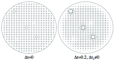
Figure 9: The site occupations for the case of Fig. 8, with the diameters of the circles proportional to the hole occupation of the sites. Note the 5 impurity sites at positions listed in the caption of Fig. 8 (three with negative potential, hence higher hole concentration) and two with positive potential, hence lower hole concentration. Note that for $\Delta t=0$ only the occupation at the impurity site changes appreciably, while for $\Delta t\neq 0$ an impurity potential of the same strength causes a much larger change of the occupation at the impurity site and occupation change also at the nearest and next nearest neighbor sites.

The reason for this large sensitivity to local perturbations can be understood from the form of the hopping amplitude Eq. (9b). A change in the local occupation will also change the hopping amplitude of a hole between that site and neighboring sites, which in turn will change the occupation of neighboring sites, and so on. In that way a local perturbation in the dynamic Hubbard model gets amplified and expanded to its neighboring region, and it is easy to understand how a non-perfect crystal will easily develop patches of charge inhomogeneity in the presence of small perturbations. These inhomogeneities cost potential (electrostatic) energy, but are advantageous in kinetic energy. The conventional Hubbard model does not exhibit this physics. There is extensive experimental evidence for charge inhomogeneities in high $T_{c}$ cupratesbianconi ; stripes ; patches ; patches2 .

VI shape effects

It is interesting to consider the effect of the shape of the sample on the charge expulsion profile in the dynamic Hubbard model. Consider an ellipsoidal shape as shown in Figure 10. The sites near the surface at the regions of higher curvature, i.e. top and bottom, have somewhat smaller hole concentration than at the regions of lower curvature at the lateral surfaces. This is easy to understand: the sites near the surface in the regions of high surface curvature have slightly lower coordination on average than those in the regions of low curvature, hence the holes do not benefit so much from kinetic energy lowering and prefer to stay away from those regions. Thinking in terms of electrons instead of holes, it means the body expels more electrons to the top and bottom than to the sides. This should give rise to a higher electric potential near the sides than at the top and bottom, and a quadrupolar electric field with field lines starting at the lateral sides and ending at the top and bottom. This is precisely the type of electric field found in the superconducting state by solving the alternative London equations proposed to describe the electrodynamics of superconductors within this theorychargeexp ; ellipsoid .

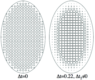
Figure 10: Effect of shape on the charge expulsion profile. $t_{h}=0.1$, $U=2$. In the ellipsoidal shape shown, for the conventional Hubbard model (left) the charge occupation near the surface is similar near the top surface and the lateral surfaces. For the dynamic Hubbard model (right) the hole concentration is somewhat higher near the lateral surfaces than near the top and bottom surfaces. For the origin of this effect, see text. Temperature is $T=0.02$.

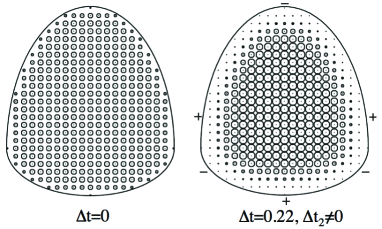
Figure 11: Same as Fig. 10 for a case where the upper half of the body is a prolate and the lower half an oblate ellipsoid of revolution. For the dynamic Hubbard model there is excess negative charge (lower hole concentration) everywhere along the surface, however there is slightly more negative charge at the top than at the bottom, as indicated by the $-$ and $+$ signs. Variations along the lateral surfaces are also indicated with $-$ and $+$ signs.

A qualitative way to understand this charge distribution in the superconducting state is the following: the electrons near the lateral surfaces can move faster than those at the top and bottom in the region of high curvature, just as racing cars. Hence they will have higher kinetic energy and consequently lower potential energy than the electrons near the top and bottom surfaces, so as to keep the same sum of kinetic and potential energies. Electrons near the lateral surfaces having lower potential energy means that the electric potential is higher near the lateral surfaces than near the top and bottom surfaces, resulting in electric field lines starting from the side and ending at the top and bottom just as found from the analysis of the hole distribution in the dynamic Hubbard model discussed in the above paragraph.

More generally, using these same arguments we expect that for other body shapes the electric potential near the surface will be higher in the regions of lower surface curvature and lower in the regions of higher surface curvature in the dynamic Hubbard model and in superconducting bodies. An example of the charge distribution for a body shape resulting from combining a prolate and an oblate ellipsoid is given in Figure 11. Examining the hole concentration in the various regions near the surface for the right panel (dynamic Hubbard model) it is seen for example that it is slightly higher near the bottom surface that has a lower curvature, than near the top surface. The resulting charge profile varies as shown by the $+$ and $-$ symbols in the figure. This is qualitatively the same pattern that was found in Ref. 100 for the electric potential for a body of this shape by solving the modified electrodynamic equations in the superconducting state.

VII charge expulsion in the superconducting state

As seen in the previous sections, the dynamic Hubbard model has a tendency to expel negative charge from its interior to the surface driven by lowering of kinetic energy. Starting with a charge neutral system in the normal state, where a uniform positive ionic charge distribution is compensated by an equal uniform negative electronic charge distribution, the negative charge expulsion would result in a net charge distribution as qualitatively shown in Fig. 3: a net excess positive charge in the interior and net excess negative charge near the surface. According to the numerical results in the previous sections (e.g. Fig. 4) the positive charge in the interior predicted by the dynamic Hubbard model Hamiltonian is approximately uniform, just as that predicted from the electrodynamic equations in the superconductorchargeexp .

This would result in the presence of an electric field in the interior of the system, that increases linearly in going from the center towards the surface. However, this cannot happen in a real normal metal since a metal in the absence of current flow cannot have a macroscopic electric field in the interior. Therefore, we conclude that longer range Coulomb interactions, omitted in the dynamic Hubbard model, prevent this from actually taking place in a real material. In other words, potential energy triumphs over kinetic energy in the normal state, and a macroscopic metal will remain charge neutral in the interior, despite the $tendency$ to develop this macroscopic charge inhomogeneity if dynamic Hubbard model physics is dominant. At most, the system will develop local charge inhomogeneity that will be screened within a Thomas Fermi length, that can be several $\AA$ in systems like underdoped high $T_{c}$ cuprates where the carrier density is very low.

However, the situation can change if the system enters the superconducting state at low temperatures. There is no a-priori reason why a superconductor cannot have an electric field in its interiorchargeexp . A superconductor is a macroscopic quantum system, and quantum systems in their ground state minimize the sum of potential and kinetic energies. That should not in general result in a uniform charge distribution that minimizes potential energy only. The electrodynamic equations that we have proposed for superconductorschargeexp predict that the superconductor has rigidity in the charge degrees of freedomchargeexp ; rigidity and will not screen an interior electric field as a normal metal would.

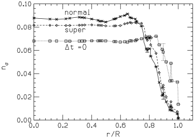
Figure 12: Comparison of occupations in the normal and superconducting states. Radius of cylinder is $R=9$, average occupation per site is $n=0.126$. $t_{h}=0.1$, $U=2$, $\Delta t=0.2$, $\Delta t_{2}=0.4$, $k_{B}T=0.02$. The average gap parameters in the superconducting state are $\Delta_{ii}=0.0044$, $\Delta_{ij}=-0.025$. We also show the occupations for the conventional Hubbard model, $\Delta t=0=\Delta t_{2}=0$. The charge expulsion is largest in the normal state of the dynamic Hubbard model.

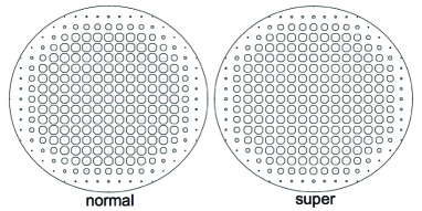
Figure 13: Real space hole occupation for the cases of Fig. 12 with $\Delta t\neq 0$. Note that the interior hole occupation is slightly $larger$ in the normal state, and the occupation near the surface slightly smaller.

To compute the charge distribution in the superconducting state we solve numerically the Bogoliubov de Gennes (BdG) equations for the dynamic Hubbard model, for systems with the same geometry as discussed in the previous sections. For the correlated hopping model ($\Delta t_{2}=0$) the equations are given in Ref. local , and are simply extended for the case $\Delta t_{2}\neq 0$. There are two gap parameters, $\Delta_{ii}$ and $\Delta_{ij}$ corresponding to on-site and nearest-neighbor pairing amplitudeslocal .

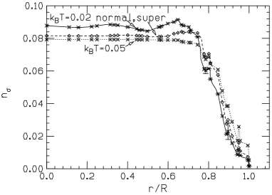
Figure 14: Dynamic Hubbard model, parameters as in Fig. 12. Comparison of occupations right above $T_{c}$, $k_{B}T=0.05$, and at $k_{B}T=0.02$, with the system in the normal (full line) and superconducting (dashed line) state. Note that when the system is allowed to go superconducting, the occupations below $T_{c}$ essentially don’t change, while if kept in the normal state the charge expulsion increases as the temperature is lowered.

We have tested our computer program by solving the BdG equations numerically on a square lattice with periodic boundary conditions and comparing with the standard BCS solution. For the cylindrical geometry with open boundary conditions considered here, the numerical solution obtained for the gap parameters deep in the interior are close to the gap parameters found in the square lattice with periodic boundary condition using both the BdG equations and the standard BCS equations applicable to translationally invariant systems. We find that the gap parameters go to zero as the surface is approached. This agrees with what was found by otherstanaka in a model with no electron-hole asymmetry in the regime of low carrier density. Here we only study the low density regime and in addition this tendency is enhanced because of the charge expulsion.

Initially we had hopedchargeexp0 that comparison of the occupations in the dynamic Hubbard model in the normal and superconducting states would yield clear evidence that the system expels negative charge from the interior to the surface as it goes superconducting, as expected on physical groundschargeexp0 ; giantatom and predicted by the electrodynamic equationschargeexp . This is $not$ what happens, as shown in Figs. 12 and 13. Instead, the charge distribution becomes more uniform in the superconducting compared to the normal state at the same temperature. In fact, it appears that as the temperature is lowered and the system enters into the superconducting state the charge expulsion that increases in the dynamic Hubbard model as the temperature is lowered in the normal state stops changing and stays essentially the same as what it is at $T_{c}$ when the system is cooled below $T_{c}$, as shown in Fig.14.

In summary, from the numerical results presented here it appears that the BCS/BdG solution of the dynamic Hubbard model does not reflect the charge expulsion predicted by the electrodynamic equations as the system enters the superconducting statechargeexp . On the other hand this is perhaps not too surprising. The charge expulsion predicted by the electrodynamic equations is of the order of 1 extra electron every $10^{6}$ sites near the surfaceelectrospin , which certainly would not be noticeable in systems of the size considered here. We have recently proposed that this predicted macroscopic charge inhomogeneity in the superconducting state should be experimentally observable through the technique of electron holographyholo1 ; holo2 ; holo3 ; holo4 .

VIII superconductivity and charge imbalance

Within the BCS formalism, the total electronic charge per site is given by

$$Q_{tot}=\frac{2}{N}\sum_{k}[u_{k}^{2}f(E_{k})+v_{k}^{2}(1-f(E_{k}))]$$ (13)

in units of the charge of one carrier, $e$ or $-e$ depending on whether one is using electron or hole representation. Eq. (13) can be written asqstar

$$Q_{tot}=Q_{c}+Q^{*}$$ (14)

with

$$Q_{c}=\frac{2}{N}\sum_{k}v_{k}^{2}$$ (15a)

the charge of the condensate, and

$$Q^{*}=\frac{2}{N}\sum_{k}(u_{k}^{2}-v_{k}^{2})f(E_{k})$$ (15b)

the average charge of the quasiparticles. The coherence factors are given by the usual form

$$u_{k}^{2}=\frac{1}{2}(1+\frac{\epsilon_{k}-\mu}{E_{k}})$$ (16a)

$$v_{k}^{2}=\frac{1}{2}(1-\frac{\epsilon_{k}-\mu}{E_{k}}).$$ (16b)

In a conventional BCS superconductor $Q^{*}=0$ in equilibrium since quasiparticles are charge neutral on average, half electron, half hole. A non-zero $Q^{*}$, termed “charge imbalance” or “branch imbalance”, can be generated in a non-equilibrium situation in the presence of current flowclarke ; tc and/or a temperature gradientps ; ct .

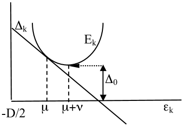
Figure 15: Gap function $\Delta_{k}$ and quasiparticle energy $E_{k}$ as a function of band energy $\epsilon_{k}$ in hole representation.

Instead, in the dynamic Hubbard model (or the correlated hopping model) a branch imbalance exists even in equilibriumthermo . The gap function has a slope of universal signdeltat

$$\Delta_{k}\equiv\Delta(\epsilon_{k})=\Delta_{m}(-\epsilon_{k}/(D/2)+c)$$ (17)

with $D$ the bandwidth and $\Delta_{m}>0$ and $c$ obtained from solution of the BCS equationsdeltat . The minimum gap is $\Delta_{0}=\Delta(\mu)/a$, with $a=\sqrt{1+(\Delta_{m}/(D/2))^{2}}$ and the quasiparticle energy is given by

$$E_{k}=\sqrt{a^{2}(\epsilon_{k}-\mu-\nu)^{2}+\Delta_{0}^{2}}.$$ (18)

The minimum gap $\Delta_{0}$ is attained not at $\epsilon_{k}=\mu$ but at $\epsilon_{k}=\mu+\nu$, with

$$\nu=\Delta_{m}(T)\Delta_{0}(T)/(aD/2)>0.$$ (19)

Both $\Delta_{0}$ and $\Delta_{m}$ go to zero at $T_{c}$ as $\sqrt{T_{c}-T}$ so $\nu$ goes to zero linearly as $T$ approaches $T_{c}$ from below. The gap function and quasiparticle excitation spectrum are shown schematically in Figure 15 in hole representation. In equilibrium, quasiparticles are symmetrically distributed around the minimum located at $\epsilon_{k}^{0}=\mu+\nu$ and as a consequence $Q^{*}>0$, quasiparticles are positively charged on average. If we ignore band edge effects we have simply

$$Q^{*}=\frac{2\nu}{N}\sum_{k}\frac{f(E_{k})}{E_{k}}$$ (20)

which is given approximately by (again ignoring band edge effects)

$$Q^{*}=\sqrt{8\pi}\frac{\nu(T)}{Da}\frac{e^{-\beta\Delta_{0}}}{(\beta\Delta_{0})^{1/2}},$$ (21)

$Q^{*}$ is suppressed at low temperatures due to the exponential factor, peaks somewhat below $T_{c}$ and goes to zero at $T_{c}$. Numerical examples are shown in ref. thermo . However when the finite bandwidth is taken into account $Q^{*}$ remains positive at $T_{c}$ and above.

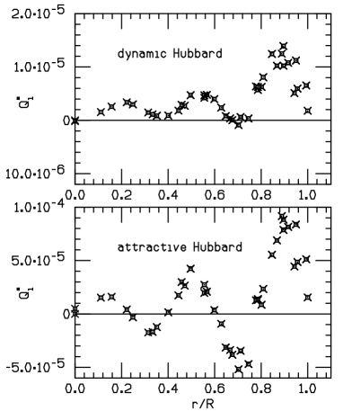
Figure 16: Quasiparticle charge (Eq. (35)) as function of distance to the center for a dynamic Hubbard model with parameters as in Fig. 12 and for an attractive Hubbard model with $t_{h}=0.1$, $U=-0.4$. Average occupation is $n=0.126$, temperature is $k_{B}T=0.01$. Note that in the dynamic Hubbard model the quasiparticle charge is predominantly positive.

Figure 16 shows the distribution as a function of the distance to the center $r$ of the quasiparticle charge $Q_{i}^{*}$ at site $i$, given by

$$Q_{i}^{*}=\frac{2}{N}\sum_{n}(u_{ni}^{2}-v_{ni}^{2})f(E_{n})$$ (22)

obtained from solution of the BdG equations, for a dynamic Hubbard model and for an attractive Hubbard model. In Eq. (22), $u_{ni}$ and $v_{ni}$ are the amplitudes of the n-th eigenvector at site $i$ obtained from diagonalization of the BdG Hamiltonianlocal , $E_{n}$ is the energy for state $n$ and $f$ is the Fermi function. In the attractive Hubbard model (Fig. 16 lower panel) particle-hole symmetry is broken only because the band is not half-full, but the interaction is particle-hole symmetric. As a consequence, the quasiparticle charge oscillates between positive and negative values. Instead, as seen in Fig. 16 (upper panel) in the dynamic Hubbard model quasiparticles are predominantly positively charged, as expected due to the shift in the chemical potential by $\nu$ displayed in Fig. 15.

Figure 17 shows the real space distribution of the quasiparticle charge in the dynamic Hubbard model (right panel). The total site occupation for this case is shown on the left panel. It can be seen from Figs. 16 and 17 that the positive quasiparticle charge is located mostly near the surface of the system. This is relevant to the discussion in the next section.

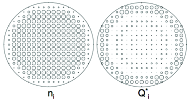
Figure 17: Real space hole occupation (left panel) and quasiparticle charge (right panel) in the superconducting state of the dynamic Hubbard model. Parameters are the same as for Figure 16 (upper panel). Note that the quasiparticle charge is predominantly near the surface of the sample.

IX two-fluid model and interior electric field

In this section we discuss to what extent the dynamic Hubbard model reflects the physics shown in Figure 3 in the superconducting state, how it depends on temperature, and how this physics could be detected experimentally.

We assume a two-fluid model, with the total carrier concentration independent of temperature. We have then

$$n_{s}=n_{s}(T)+n_{n}(T)$$ (23)

with $n_{s}$ the total carrier (hole) concentration and $n_{s}(T)$ and $n_{n}(T)$ the superfluid and normal components at $0\leq T\leq T_{c}$. Within the two-fluid interpretation of BCS theory they are given in terms of the London penetration depth as

$$n_{s}(T)=n_{s}\frac{\lambda_{L}^{2}}{\lambda_{L}^{2}(T)}$$ (24a)

$$n_{n}(T)=n_{s}\lambda_{L}^{2}(\frac{1}{\lambda_{L}^{2}}-\frac{1}{\lambda_{L}(T)^{2}})$$ (24b)

with $\lambda_{L}$ ($\lambda_{L}(T)$) the London penetration depths at zero (finite) temperature. Ignoring finite bandwidth effects the quasiparticle density is thentinkham

$$n_{n}(T)=2n_{s}\int_{\Delta_{0}}^{\infty}dE(-\frac{\partial f}{\partial E})\frac{E}{\sqrt{E^{2}-\Delta_{0}^{2}}}$$ (25)

which yields at low temperatures

$$n_{n}(T)=\sqrt{2\pi}(\beta\Delta_{0})^{1/2}e^{-\beta\Delta_{0}}n_{s}.$$ (26)

On the other hand, the average quasiparticle charge per site is given by Eq. (21). Combining with Eq. (26),

$$\frac{Q^{*}(T)}{n_{n}(T)}=\frac{1}{a}\frac{k_{B}T}{D/2}\frac{\nu}{\Delta_{0}}=\frac{k_{B}T\Delta_{m}}{\Delta_{m}^{2}+(D/2)^{2}}\sim\frac{k_{B}T\Delta_{m}}{(D/2)^{2}}.$$ (27)

It can be seen that the quasiparticle charge is a small fraction of the quasiparticle density. For example, for the parameters of Fig. 16 we have

$$D=2z(t_{h}+n\Delta t+\frac{n^{2}}{4}\Delta t_{2})=1.01,$$ (28)

$\Delta_{ij}=0.00253$, $\Delta_{m}=z\Delta_{ij}=0.10$, hence $Q^{*}/n_{n}=0.004$.

Assuming the system as a whole is charge neutral, the negative charge of the electrons in the band exactly compensates the positive charge of the ions, which is uniformly distributed in space (except for variations on the scale of $\AA$). At temperatures below $T_{c}$, the quasiparticles have a net positive charge, hence as a consequence the condensate has a total negative charge $greater$ than the total positive charge of the ions. The condensate is highly mobile, and just as in a normal metal any excess negative charge will move to the surfacethomson it is natural to expect that negative charge from the condensate will move to the surface.

Furthermore, we have seen in the previous section that the positive quasiparticle charge is located predominantly near the surface in the superconducting state (Fig. 17 right panel). This can be interpreted as reflecting the fact that the superfluid has higher negative density near the surface, and the positive normal fluid consequently develops higher density near the surface to screen the superfluid charge. In addition, as already seen in the normal state of the dynamic Hubbard model, the total hole concentration is smaller near the surface which implies extra negative charge near the surface. Thus we argue that the dynamic Hubbard model provides support to the prediction of the electrodynamic equations of the theorychargeexp0 ; chargeexp that the superconductor expels superfluid negative charge from the interior to the surface.

Whether or not a macroscopic electric field will exist in the interior of the superconductor depends on whether there are enough quasiparticles to screen the electric field created by the negative charge expulsion of the condensate. In the ground state (no quasiparticles) the theory predicts that the net positive charge density in the interior iselectrospin

$$\rho_{0}=\frac{r_{q}}{R}|e|n_{s}=\rho_{s}+\rho_{ions}$$ (29)

with $R$ the radius of the cylinder and $r_{q}=\hbar/(2m_{e}c)=0.00193\AA$ the quantum electron radius, and there is a negative charge density

$$\rho_{-}=-\frac{R}{2\lambda_{L}}\rho_{0}=\rho_{s}+\rho_{ions}$$ (30)

within a London penetration depth of the surface, as shown schematically in Fig. 3. The charge densities at zero temperature are shown schematically in the left panels of Figure 18. $\rho_{s}$ denotes the superfluid charge density.

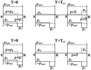
Figure 18: Charge distribution in the superconductor (schematic). In the ground state (left panels) there is an excess positive charge density $\rho_{0}$ in the interior and an excess negative charge density $\rho_{-}$ near the surface. At low temperatures $T<T_{cr}$ (upper panels) the charge density is partially screened by excited quasiparticles but a net positive charge density $\rho>0$ remains in the interior and a net negative charge density $\rho<0$ near the surface (dot-dashed lines in upper right panel). At temperature $T=T_{cr}$ and above the net charge density is zero both in the interior and near the surface.

At finite temperatures, there is a positive quasiparticle charge density excited, $\rho_{n}=|e|Q^{*}$, and a crossover temperature $T_{cr}$ can be defined. For temperatures lower than $T_{cr}$, the average quasiparticle charge density excited is smaller than $\rho_{0}$. In the middle top panel of Fig. 18 we assume $\rho_{n}$ is uniformly distributed, and in the right top panel we assume all $\rho_{n}$ has moved to within the London penetration depth of the surface. Even so, it is unable to screen the internal electric field, since a positive net charge density $\rho=\rho_{0}-\rho_{n}>0$ remains in the interior and a negative net charge density $\rho<0$ remains near the surface, as shown in the top right panel of Fig. 18. At the crossover temperature $T_{cr}$ the quasiparticle charge density excited reaches the value $\rho_{0}$, and by migrating to the region within a London penetration depth of the surface (lower right panel of Fig. 18) it can completely screen both the interior positive charge and the negative charge in the surface layer, so that the electric field everywhere gets cancelled. This will also be the case at any temperature $T>T_{cr}$.

The value of the crossover temperature can be obtained from the equation

$$Q^{*}=\frac{Q^{*}}{n_{n}}n_{n}=\frac{r_{q}}{R}n_{s}$$ (31)

with $Q^{*}/n_{n}$ given by Eq. (27) and $n_{n}$ given by Eq. (26), hence

$$\frac{k_{B}T_{cr}\Delta_{m}}{(D/2)^{2}}(\frac{2\pi\Delta_{0}}{k_{B}T_{cr}})^{1/2}e^{-\Delta_{0}/(k_{B}T_{cr})}=\frac{r_{q}}{R}.$$ (32)

For example, assuming the usual relation $2\Delta_{0}/k_{B}T_{c}=3.53$, for the case under consideration with $Q^{*}/n_{n}=0.004$ and assuming $R=500nm$ yields $T_{cr}=0.16T_{c}$. For temperatures lower than $T_{cr}$, a nonzero electric field is predicted to exist in the interior of the superconductor.

In the presence of a non-zero internal electric field, superconductors of non-spherical shape should also develop electric fields extending to the region exterior to the body, of magnitude and direction determined by the shape of the body and the electrodynamic equations of the superconductorellipsoid ; 100 . These electric fields should be experimentally detectable in the neighborhood of superconductors at temperature lower than $T_{cr}$. In addition, the internal electric field should be directly detectable in electron holography experimentsholo1 ; holo2 ; holo3 . The magnitude of these predicted electric fields is of order of $H_{c1}$, the lower critical magnetic field, in the interior of the superconductorelectrospin , and an appreciable fraction of it in the region outside the superconductor near the surface, depending on the shape of the bodyellipsoid ; 100 . No external electric field is expected outside a planar surface or a spherical body.

X the Meissner effect, the London moment and the gyromagnetic effect

The fact that in superconductors the superfluid carries negative charge is established experimentally from experiments that measure the London momentlm1 ; lm2 : a rotating superconductor develops a magnetic field that is always parallel, never antiparallel, to the direction of the mechanical angular momentum of the bodyehasym .

We have seen that the dynamic Hubbard model has a tendency to expel negative charge, that in a real system is inhibited in the normal state because of the effect of long-range Coulomb repulsion but may take place when the system becomes superconducting. The considerations in the previous section suggest that as a system becomes superconducting the electrons that condense into the superfluid state are partially expelled towards the surface, and at the same time normal electrons flow inward to compensate for the charge imbalance, as indicated by the fact that the positive quasiparticle charge moves outward in the superconducting state as seen in the last section.

Consider now these processes in the presence of an external magnetic field in the $z$ direction, as shown in Fig. 19. The outflowing superfluid electrons will be deflected counterclockwise by the Lorentz force exerted by the magnetic field, building up a Meissner current flowing clockwise near the surface that suppresses the applied field in the interior. At the same time, the inflowing normal electrons are deflected clockwise by the magnetic field. Because these electrons undergo scattering from the ions, they will transmit their momentum to the ions and the body as a whole will start rotating in a clockwise direction. And because these electrons are slowed down and ultimately stopped by the collisions with the ions they will not reinforce the applied magnetic field. The end result is a superfluid current near the surface flowing in clockwise direction (i.e. superfluid electrons flowing in counterclockwise direction) that suppresses the interior magnetic field, and a slow body rotation in the clockwise direction that exactly cancels the mechanical angular momentum carried by the superfluid electrons in the Meissner current, as required by angular momentum conservation.

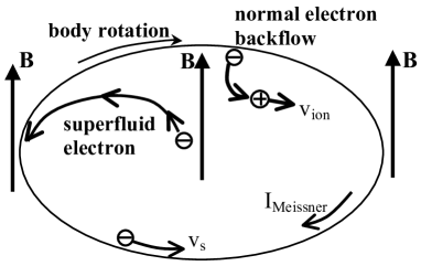
Figure 19: The outflowing superfluid electrons are deflected in the counterclockwise direction by the applied magnetic field, generating a clockwise Meissner current ($I_{Meissner}$) near the surface that suppresses the magnetic field in the interior. The inflowing normal electrons collide with the ions and impart the entire body with angular momentum antiparallel to the applied magnetic field, that is equal and opposite to the mechanical angular momentum of the electrons in the Meissner current.

The magnetic field generated by rotating superconductors (London moment)lm1 ; lm2 can be similarly explainedspincurrent by the fact that in a rotating normal metal that is cooled into the superconducting state the expelled superfluid electrons, that are moving at the same angular velocity as the body, will have a smaller tangential velocity than the body when they reach the surface, giving rise to a net current and resulting magnetic moment in direction $parallel$, never antiparallel, to the angular momentum of the rotating body.

More quantitatively, the outflow occurs because superfluid electrons expand their orbits from microscopic radius $k_{F}^{-1}$ to mesoscopic radius $2\lambda_{L}$sm , in the process acquiring an azimuthal velocityazim

$$v_{\phi}=-\frac{e}{2m_{e}c}r=-\frac{e}{m_{e}c}\lambda_{L}B$$ (33)

which is the speed of the superfluid electrons in the Meissner currenttinkham . The total mechanical angular momentum acquired by these electrons in a cylinder of radius $R$ and height $h$ is

$$L_{el}=\pi R^{2}hn_{s}(m_{e}v_{\phi}2\lambda_{L})$$ (34)

which coincides with the total electronic angular momentum of the Meissner current flowing within a London penetration depth of the surface

$$L_{Meissner}=2\pi R\lambda_{L}hn_{s}(m_{e}v_{\phi}R).$$ (35)

The inflowing normal electrons transmit the same angular momentum to the body as a whole by collisions with the ions, as required by angular momentum conservationangmom1 . As a consequence, the body starts rotating with angular velocity determined by the condition of angular momentum conservation, as measured experimentallygyro1 ; gyro2 ; gyro3 (gyromagnetic effect).

These processes provide an intuitive explanation for the dynamics of the Meissner effectsm , the generation of the London moment, the gyromagnetic effect and the puzzle of angular momentum conservationangmom1 ; angmom2 in superconductors, $provided$ the superconductor is described by a dynamic Hubbard model that gives rise to negative charge expulsion. In contrast, in superconductors not described by dynamic Hubbard models but by conventional BCS-electron-phonon theorytinkham no charge expulsion takes place and hence these considerations don’t apply. For those superconductors, if they exist, the dynamical origins of the Meissner effect and the London moment and the explanation of the angular momentum puzzle remain to be elucidated.

XI discussion

Both the conventional Hubbard model and the dynamic Hubbard model are simplified descriptions of real materials, and whether or not they contain the physics of interest for particular real materials is in principle an open question. In this paper we have argued that the new physics that the dynamic Hubbard model incorporates beyond what is contained in the conventional Hubbard model is key to understanding many properties of high $T_{c}$ cuprates as well as of superconductors in general.

The new physics of the dynamic Hubbard model is that it allows the electronic orbital to expand when it is doubly occupied, as it occurs in real atoms. This expansion has associated with it outward motion of negative charge as well as lowering of the electron’s kinetic energy at the atomic level, and it is of course electron-hole $asymmetric$ (the orbital does not change when a second $hole$ is added to a non-degenerate orbital occupied by one hole). In the conventional Hubbard model instead, the state of the first electron in the orbital does not change when a second electron is added, the kinetic energy of the electron does not change (the potential energy does), and the model is electron-hole symmetric.

We have argued in this paper and in previous work that these three properties that occur already at the atomic level in the dynamic Hubbard model, negative charge expulsion, lowering of electronic kinetic energy, and electron-hole asymmetry, are key to understanding high $T_{c}$ superconductivity in the cuprates and superconductivity in general. Furthermore we have shown in this paper that these properties are also displayed by the entire system described by a dynamic Hubbard model in the normal state.

The tendency of the dynamic Hubbard model to expel negative charge and the tendency to pairing of holes and superconductivity driven by kinetic energy lowering of course go hand in hand: they both originate in the fact that the kinetic energy of a hole is lowered when another hole is nearby. Increasing the chance of having another hole nearby can be achieved by negative charge expulsion, thus increasing the $overall$ hole density, and by pairing, thus increasing the $local$ hole density. The propensity of dynamic Hubbard models to develop charge inhomogeneity and the high sensitivity to disorder of the local superconducting gap found in earlier worklocal also go hand in hand, since both originate in the fact that the kinetic energy varies with charge occupation, which is what gives rise to a kinetic-energy-dependent pair interaction and superconducting gap functiondeltat .

We restricted ourselves in this paper to the antiadiabatic limit, i.e. assuming that the energy scale associated with the orbit expansion ($\omega_{0}$ in Eq. (4)) is sufficiently large than it can be assumed infinite. This brings about the simplification that the high energy degrees of freedom can be eliminated and the Hamiltonian becomes equivalent to the low energy effective Hamiltonian Eq. (7), a Hubbard model with correlated hoppings, linear and nonlinear terms $\Delta t$ and $\Delta t_{2}$. This low energy effective Hamiltonian, together with the quasiparticle weight renormalization described by Eq. (6), describes many properties that we believe are relevant to real materials and are not described by the conventional Hubbard model. In particular it gives rise to hole superconductivitydeltat , driven by lowering of kinetic energy of the carriersapparent ; kinetic , with many characteristic features that resemble properties of the cuprates. In other work we have also examined the effect of the high energy degrees of freedom in describing spectral weight transfer from high to low energies (“undressing”undr ) as the number of holes increases and as the system enters the superconducting state, as well as the effect of finite $\omega_{0}$ in further promoting pairing in this modeldynfrank .

The effects predicted by this Hamiltonian are largest when the coupling constant $g$ is large, or equivalently when the overlap matrix element $S$ is small, which corresponds to a “soft orbital” that would exist for negatively charged anions, $and$ the effects are also largest when the band is almost full with negative electrons (strong coupling regime)strong . Thus, not surprisingly, more negative charge at the ion or/and in the band yield larger tendency to negative charge expulsion for the entire system. We believe that the Hamiltonian is relevant to describe the physics of superconductors including high $T_{c}$ cuprates, $Fe$ pnictides, $Fe$ chalcogenides, $MgB_{2}$ and $BiS_{2}$-basedbis2 superconductors. These materials have negatively charged ions ($O^{--},As^{---},S^{--},Se^{--},B^{-}$) with soft orbitals, and for most of them, including “electron-doped” cupratesedoped , there is experimental evidence for dominant $hole$ transport in the normal state. We suggest that the orbital expansion and contraction of these negative ions depending on their electronic occupation is responsible for many interesting properties of these materials including their superconductivity, and is described by the dynamic Hubbard model.

We have also examined here the question whether the interiorchargeexp and exteriorellipsoid electric fields predicted to exist in the ground state of superconductors within this theory would exist also at finite temperatures and concluded that they should exist and hence be experimentally detectable up to a crossover temperature $T_{cr}$, calculated to be $0.16T_{c}$ in one example. We also examined the effect of the body shape (surface curvature) on the charge distribution near the surface in the normal state of the model and found that it is consistent with the pattern of electric field dependence on particle shape predicted in the superconducting stateellipsoid ; 100 .

Finally, we have proposed that the negative charge expulsion predicted by dynamic Hubbard models is relevant to the understanding of the Meissner effect, the London moment and the gyromagnetic effect exhibited by all superconductors.

In summary, we argue that it is remarkable that the dynamic Hubbard model exhibits the same physics at the level of the single atom and of the system as a whole, and both in the normal and in the superconducting states, and that the same physics is found in different ways through seemingly different physical arguments and mathematical equations. In particular, we hope the reader will appreciate the remarkable qualitative similarity of Figs. 1, 2 and 3, depicting the charge distribution in an atom, a system in the normal state and a superconductor within this model. Superconductors have been called “giant atoms” in the early days of superconductivity for many $other$ reasonsga1 ; ga2 ; ga3 . The essential property of the atom, that it is $not$ electron-hole symmetric because the negative electron is much lighter than the positive nucleus, manifests itself in the atom described by the dynamic Hubbard model and in the state of a macroscopic superconducting body described by the model, and is missed in the world described by particle-hole symmetric conventional Hubbard or Fröhlich models both at the atomic level and at the level of the macroscopic superconductor. The superconductor closely resembles a “giant atom” within our description, with the highly mobile light negative superfluid reflecting the atomic electron, and the heavy positive quasiparticles reflecting the positive nucleus.

Much of the physics of dynamic Hubbard models for finite $\omega_{0}$ remains to be understood. In fact, the model itself may require substantial modification to account for different values of $\omega_{0}$ for different electronic occupations: the excitation spectrum of the neutral hydrogen atom, $H$, is certainly very different from that of $H^{-}$. In connection with this and going beyond the antiadiabatic limit where only diagonal transitions of the auxiliary boson field are taken into account as in this paper, it is possible that $vertical$ transitions may play a key role in describing the superconducting stateeh3 . It is also an open question to what extent dynamic Hubbard models can describe the mysterious “pseudogap state” of underdoped high $T_{c}$ cuprate materials. These and other questions will be the subject of future work.

References

- (1) J.C. Slater, Quantum Theory of Atomic Structure, McGraw-Hill, New York, 1960.
- (2) “The Hubbard Model: A Collection of Reprints”, ed. by A. Montorsi, World Scientific, Singapore, 1992.
- (3) “The Hubbard model: its physics and mathematical physics”, ed. by D. Baeriswyl, D.K. Campbell, J.M.P. Carmelo, F. Guinea and E. Louis, NATO ASI Series B Vol. 343, Plenum, New York, 1995.
- (4) Hirsch JE 1994 Inapplicability of the Hubbard model for the description of real strongly correlated electrons. Physica B 199&200: 366-372
- (5) Hirsch JE (2002) Why holes are not like electrons: A microscopic analysis of the differences between holes and electrons in condensed matter. Phys. Rev. B 65: 184502.
- (6) Hirsch J E 1989 Hole Superconductivity. Phys.Lett. A 134: 451-455.
- (7) Hirsch J E, Tang S 1989 Hole superconductivity in oxides. Sol.St. Comm. 69: 987-989.
- (8) Hirsch J E 2001 Dynamic Hubbard Model. Phys.Rev. Lett. 87: 206402.
- (9) Hirsch J E 1991 Pairing of holes in a tight binding model with repulsive Coulomb interactions. Phys. Rev. B 43: 11400-11403.
- (10) Pincus P 1972 Polaron effects in the nearly atomic limit of the Hubbard model. Solid St. Comm. 11: 51-54.
- (11) Fortunelli A, Painelli A 1993 Interacting electrons in the solid state: the role of orbital relaxation. Chem. Phys. Lett. 214: 402-408.
- (12) Hirsch J E 2001 Consequences of charge imbalance in superconductors within the theory of hole superconductivity. Phys. Lett. A 281: 44-47.
- (13) Hirsch JE 2003 Charge expulsion and electric field in superconductors. Phys. Rev. 68: 184502; 2004 Electrodynamics of superconductors. Phys. Rev. 69: 214515.
- (14) See the website http://physics.ucsd.edu/ jorge/hole.html for a list of references.
- (15) Hirsch JE 2006 The fundamental role of charge asymmetry in superconductivity. Jour. Phys. Chem. Solids 67: 21-26 and references therein
- (16) Hirsch J E, Marsiglio F 1989 Superconducting state in an oxygen hole metal. Phys. Rev. B 39: 11515-11525; 1993 London penetration depth in hole superconductivity. Phys. Rev. 45: 4807-4818; Marsiglio F, Hirsch J E 1990 Hole superconductivity and the high Tc oxides. Phys. Rev. B 41: 6435-6456.
- (17) Hirsch J E 1992 Apparent violation of the conductivity sum rule in certain superconductors. Physica C 199: 305-310.
- (18) Hirsch J E, Marsiglio F 2000 Where is 99 of the condensation energy of coming from? Physica C 331: 150-156.
- (19) Hirsch J E, Marsiglio F 2000 Optical sum rule violation, superfluid weight and condensation energy in the cuprates. Phys. Rev. B 62: 15131-15150.
- (20) Hirsch J E 2003 Superconductors as giant atoms predicted by the theory of hole superconductivity. Phys. Lett. A 309, 457-464.
- (21) Marsiglio F, Hirsch J E 1989 Tunneling asymmetry: a test of superconductivity mechanisms. Physica C 159: 157-160.
- (22) Hirsch JE 1994 Thermoelectric power of superconductive tunnel junctions. Phys. Rev. Lett. 72: 558-561.
- (23) Hirsch J E 2003 Electron-hole asymmetry and superconductivity. Phys. Rev. B 68: 012510.
- (24) F. London, in “Report of an International Conference on fundamental particles and low temperatures”, Taylor and Francis, London, p. 1.
- (25) F. London has written a two-volume book series entitled ‘Superfluids’ (Wiley, New York), Volume I (1950) on superconductors and Volume II (1954) on superfluid , emphasizing many common aspects of the phenomena.
- (26) Hirsch J E 2011 Kinetic energy driven superconductivity and superfluidity. Mod. Phys. Lett. B 25: 2219-2237.
- (27) Hirsch J E 2013 Charge expulsion, charge inhomogeneity, and phase separation in dynamic Hubbard models. Phys.Rev. B 87: 184506.
- (28) Bianconi A et al 2000 The stripe critical point for cuprates. Jour. of Phys. Cond. Matt. 12: 10655-10666.
- (29) Kivelson S A et al 2003 How to detect fluctuating stripes in the high-temperature superconductors. Rev. Mod. Phys. 75: 1201-1241.
- (30) Pan S H et al 2001 Microscopic electronic inhomogeneity in the high-Tc superconductor Bi2Sr2CaCu2O8+x. Nature 413: 282-285.
- (31) Kohsaka Y et al 2012 Visualization of the emergence of the pseudogap state and the evolution to superconductivity in a lightly hole-doped Mott insulator. Nature Physics 8: 534-538.
- (32) Bardeen J 1955 Theory of the Meissner Effect in Superconductors. Phys. Rev. 97: 1724-1725.
- (33) Matsubara T 1955 A General Theory of Meissner Effect. Prog. Theor. Phys. 13: 631-632.
- (34) Bardeen L. N., Cooper L N and Schrieffer J R 1957 Theory of Superconductivity. Phys. Rev. 108: 1175-1204.
- (35) P. W. Anderson P W 1958 Coherent Excited States in the Theory of Superconductivity: Gauge Invariance and the Meissner Effect. Phys. Rev. 110: 827-835.
- (36) Rickayzen G 1958 Meissner Effect and Gauge Invariance. Phys. Rev. 111: 817-821; 1959 Collective Excitations and the Meissner Effect. Phys. Rev. Lett. 2: 90-91; 1959 Collective Excitations in the Theory of Superconductivity. Phys. Rev. 115: 795-808.
- (37) Wentzel G 1958 Meissner Effect. Phys. Rev. 111: 1488-1492; 1959 Problem of Gauge Invariance in the Theory of the Meissner Effect. Phys. Rev. Lett. 2: 33-34.
- (38) Pines D and Schrieffer JR 1958 Theory of the Meissner Effect. Phys. Rev. Lett. 1: 407-408.
- (39) May R M, Schafroth M R 1959 Meissner-Ochsenfeld Effect in the Bogoljubov Theory. Phys. Rev. 115: 1446-1459.
- (40) Nambu Y 1960 Quasi-Particles and Gauge Invariance in the Theory of Superconductivity. Phys. Rev. 117: 648-663.
- (41) Kadanoff L P, Martin P C 1961 Theory of Many-Particle Systems. II. Superconductivity. Phys. Rev. 124: 670-697.
- (42) Uhlenbrock D A, Zumino B 1964 Meissner Effect and Flux Quantization in the Quasiparticle Picture. Phys. Rev. 133: A350-A361.
- (43) Hirsch J E 2003 The Lorentz force and superconductivity. Phys. Lett. A 315: 474-479..
- (44) Hirsch J E 2009 BCS theory of superconductivity: it is time to question its validity. Physica Scripta 80: 035702.
- (45) Hirsch J E 2010 Electromotive forces and the Meissner effect puzzle, J.E. Hirsch, Jour. Sup. Nov. Mag. 23, 309-317.
- (46) Hirsch J E 2012 The origin of the Meissner effect in new and old superconductors. Physica Scripta 85: 035704.
- (47) Newcomb W A 1958 Motion of magnetic lines of force. Ann. Phys. 3: 347-385.
- (48) Cohen M L 2010 Predicting and explaining Tc and other properties of BCS superconductors. Phys. Lett. B 24: 2755-2768.
- (49) Norman M R The Challenge of Unconventional Superconductivity. Science 332: 196-200.
- (50) I. Newton, “The Mathematical Principles of Natural Philosophy”, University of California Press, Berkeley, 1999.
- (51) Hirsch J E 2003 Electronic dynamic Hubbard model: exact diagonalization study. Phys. Rev. B 67: 035103.
- (52) Hirsch J E 1992 Superconductors that change color when they become superconducting. Physica C 201: 347-361.
- (53) Hirsch J E 1993 Polaronic superconductivity in the absence of electron-hole symmetry. Phys. Rev. B 47: 5351-5358.
- (54) Hirsch J E 2000 Superconductivity from Undressing. Phys. Rev. B 62: 14487-14497.
- (55) J.D. Mahan, “Many Particle Physics”, Third Edition, Plenum, New York, 2000.
- (56) Hirsch J E 2000 Superconductivity from Undressing. II. Single Particle Green’s Function and Photoemission in Cuprates. Phys. Rev. B 62: 14998.
- (57) Hirsch J E 2001 Superconductivity from Hole Undressing. Physica C 364-365: 37-42.
- (58) Hirsch J E 2002 Quantum Monte Carlo and exact diagonalization study of a dynamic Hubbard model. Phys. Rev. B 65: 214510; Quasiparticle undressing in a dynamic Hubbard model: exact diagonalization study. Phys. Rev. B 66: 064507.
- (59) S Kivelson S, Su W P, Schrieffer J R and Heeger A. J. 1987 Missing bond-charge repulsion in the extended Hubbard model: Effects in polyacetylene. Phys. Rev. Lett. 58: 1899-1902.
- (60) Campbell D K, Tinka Gammel J and Loh E Y 1988 Bond-charge coulomb repulsion in peierls-hubbard models. Phys. Rev. B 38: 12043-12046.
- (61) Micnas R, Ranninger J and Robaszkiewicz S. 1990 Superconductivity in narrow-band systems with local nonretarded attractive interactions. Rev. Mod. Phys. 62: 113-171.
- (62) Bariev R Z et al 1993 Exact solution of a one-dimensional model of hole superconductivity. Jour. Phys. A 26: 1249-1257.
- (63) Arrachea L et al 1994 Superconducting correlations in Hubbard chains with correlated hopping. Phys. Rev. B 50: 16044-16051.
- (64) Airoldi M, and Parola A 1995 Superconducting ground state in a model with bond-charge interaction. Phys. Rev. B 51: 1632716335.
- (65) Marsiglio F, Teshima R and Hirsch J E. Dynamic Hubbard model: Effect of finite boson frequency. Phys. Rev. B 68: 224507.
- (66) Hirsch J E 1992 Effect of local potential variations in the model of hole superconductivity. Physica C 194: 119-125.
- (67) Hirsch J E 2004 Predicted electric field near small superconducting ellipsoids. Phys.Rev. Lett. 92: 016402.
- (68) Hirsch J E 2012 Correcting 100 years of misunderstanding: electric fields in superconductors, hole superconductivity, and the Meissner effect. Jour. Supercond. Novel Mag. 25: 1357-1360.
- (69) Hirsch J E 2012 Experimental consequences of predicted charge rigidity of superconductors. Physica C 478: 42-48.
- (70) Tanaka K, Marsiglio F 2003 S-wave superconductivity near a surface. Physica C 478: 356-368.
- (71) Hirsch J E 2008 Electrodynamics of spin currents in superconductors. Ann. der Physik (Berlin) 17: 380-409.
- (72) Hirsch J E 2013 Prediction of unexpected behavior of the mean inner potential of superconductors. Physica C 490: 1-4.
- (73) Hirsch J E 2013 Apparent increase in the thickness of superconducting particles at low temperatures measured by electron holography. Ultramicroscopy 133, 67-71.
- (74) Hirsch J E 2013 Superconductivity, diamagnetism, and the mean inner potential of solids. arXiv:1307.4438.
- (75) A. Tonomura, “Electron Holography”, Springer, Berlin, 1999.
- (76) Kadin A M, Smith L N and Skocpol W J 1980 Charge imbalance waves and nonequilibrium dynamics near a superconducting phase-slip center. J. Low Temp. Phys. 38: 497-534.
- (77) Clarke J 1972 Experimental Observation of Pair-Quasiparticle Potential Difference in Nonequilibrium Superconductors. Phys. Rev. Lett. 28: 1363-1366.
- (78) Tinkham M, Clarke J 1972 Theory of Pair-Quasiparticle Potential Difference in Nonequilibrium Superconductors. Phys. Rev. Lett. 28: 1366- -1369.
- (79) Pethick C, Smith H 1972 Generation of Charge Imbalance in a Superconductor by a Temperature Gradient. Phys. Rev. Lett. 43: 640-642.
- (80) Clarke J et al 1979 Branch-imbalance relaxation times in superconductors. Phys. Rev. B 20: 3933-3937.
- (81) M. Tinkham, “Introduction to Superconductivity”, 2nd ed, McGraw Hill, New York, 1996.
- (82) Levin Y, Arenzon J J 2003 Why charges go to the surface: A generalized Thomson problem. Europhys. Lett. 63: 415-418.
- (83) Hildebrand A F 1964 Magnetic Field of a Rotating Superconductor. Phys. Rev. Lett. 8: 190-191.
- (84) Verheijen A A et al 1990 Measurement of the London moment in two high-temperature superconductors. Nature 345: 418-419.
- (85) Hirsch J E 2005 Spin currents in superconductors. Phys. Rev. B 71: 184521.
- (86) Hirsch J E 2008 Spin Meissner Effect in Superconductors and the Origin of the Meissner Effect. Europhys. Lett. 81: 67003.
- (87) Hirsch JE 2009 Charge expulsion, Spin Meissner effect, and charge inhomogeneity in superconductors. Jour. Sup. Nov. Mag. 22, 131-139.
- (88) Hirsch JE 2007 Do superconductors violate Lenz’s law? Body rotation under field cooling and theoretical implications. Phys. Lett. A 366: 615-619.
- (89) Kikoin I K and Gubar S W 1940 Gyromagnetic effects in super conductors. J. Phys. USSR 3: 333-354.
- (90) Pry R H, A.L. Lathrop A L and Houston W V 1952 Gyromagnetic Effect in a Superconductor. Phys. Rev. 86: 905-907.
- (91) Doll R 1958 Messung des gyromagnetischen Effektes an makroskopischen und mikroskopischen, supraleitenden Bleikugeln. Z. Phys. 153: 207-236.
- (92) Hirsch J E 2008 The missing angular momentum of superconductors. Jour. Phys. Cond. Matt. 20: 235233.
- (93) Hirsch J E 2000 Hole superconductivity from kinetic energy gain Physica C 341-348: 213-216.
- (94) Marsiglio F, Hirsch J E 1990 Superconductivity in oxides: from strong to weak coupling. Physica C 165: 71-76.
- (95) Mizuguchi Y et al 2012 Superconductivity in Novel BiS2-Based Layered Superconductor LaO1-xFxBiS2. J. Phys. Soc. Jpn. 81: 114725.
- (96) Jiang W et al 1994 Anomalous Transport Properties in Superconducting Nd1.85Ce0.15CuO4 ?. Phys. Rev. Lett. 73: 1291-1294); Fournier P et al 1997 Thermomagnetic transport properties of Nd1.85Ce0.15CuO4+? films: Evidence for two types of charge carriers. Phys. Rev. B 56: 14149-14156; Dagan Y, Greene R L 2007 Hole superconductivity in the electron-doped superconductor Pr2?xCexCuO4. Phys. Rev. B 76: 024506.
- (97) London F, London H 1935 Supraleitung und diamagnetismus. Physica 2: 341-354.
- (98) H Smith H G, Wilhelm J O 1935 Superconductivity. Rev. Mod. Phys. 4: 237-271.
- (99) Ginsburg W L, Vogel H 1953 Der gegenwärtige Stand der Theorie der Supraleitung. Fortschritte der Physik 1: 101-163.
- (100) Hirsch J E 2009 Why holes are not like electrons. III. How holes in the normal state turn into electrons in the superconducting state. Int. J. Mod. Phys. 23: 3035-3057.