Optical conductivity for the surface of a Topological Insulator

Abstract

The optical conductivity for the surface excitations for a Topological Insulator as a function of the chemical potential and disorder is considered. Due to the time reversal symmetry the chiral metallic surface states are protected against disorder. This allow to use the averaged single particle Green’s function to compute the optical conductivity. We compute the conductivity in the limit of a finite disorder. We find that the conductivity as a function of the chemical potential $\mu$ and frequency $\Omega$ is given by the universal value $\sigma(\Omega>2\mu)=\frac{e^{2}\pi}{8h}$. For frequencies $\Omega<\mu$ and elastic mean free path $l_{el}=v\tau$ which obey $k_{F}l>1$ we obtain the conductivity is given by $\sigma(\Omega<2|\mu|)=\frac{e^{2}}{2h}\frac{k_{F}l_{el}}{(\Omega\tau)^{2}+1}$. In the limit of zero disorder we find $\sigma(\mu\neq 0,\Omega,k_{F}l\rightarrow\infty)=\frac{e^{2}\pi}{2h}|\mu|\delta(\Omega)$.

I. Introduction

For time reversal invariant systems one finds that for Kramer’s states the time reversal operator $\vartheta$ obey $\vartheta^{2}=-1$ and thus the second Chern number is given by $(-1)^{\nu}=-1$ where $\nu$ is an odd number. $Topological$ $Insulators$ $(TI)$ Volkov ; Kane ; Zhang ; David are characterized by chiralic gapless electronic spectrum. For the $3D$ $TI$ material $Bi_{2}Se_{3}$ the surface state consist of a $Weyl$ equation with single Dirac Cone which is below the chemical potential $\mu$ and the bulk gap $0.3eV$. Due to the topology the backscattering is suppressed Balatzky and therefore localization might be prohibited. Tunneling scanning has confirmed the presence of backscattering and therefore the presence of a topological metallic state. The conductivity results are less conclusive, due the presence of the $3D$ bulk gap Culcer or the insulating gap for thin layers $TI$. The charge current operator for Weyl equation is identified with the spin on the surface of the $TI$. Therefore for clean systems conservation of momentum will cause the low frequency conductivity to vanish, only the optical conductivity for frequency $\Omega>2\mu$ ($\mu$ is the chemical potential) is finite. In the presence of impurities elastic scattering conserve energy but not the quasi momentum, giving rise to a finite Drude conductivity. Due to the spin orbit interaction anti-localization effects dominate the physics giving rise to a metallic conductivity Hikami ; Ando ; Stern ; Shen ; Hankiewicz . For the Weyl equation the velocity operator is given by: $\frac{dr^{i}}{dt}=v_{F}\epsilon_{i,j}\sigma^{j}$and ,$i,j=1,2$ and the charge current is given by the spin operator. We formulate the optical conductivity for a finite chemical potential. We define Green’s functions for particles and anti-particles (holes). Our results are as as following: For a finite chemical potential we find $\sigma(\Omega>2\mu)=\frac{e^{2}\pi}{8h}[\mu+\frac{1}{4}f_{F.D.}(-\Omega+\mu)]$ which at low temperature takes the universal value $\sigma(\omega>\mu)=\frac{e^{2}\pi}{8h}$. The results obtained here in the absence of disorder are similar to the one obtained in graphene Ziegler . For weak disorder and chemical potential $\mu>\Omega$ we find the that the conductivity is given by the Drude conductivity, $\sigma(\Omega<2|\mu|)=\frac{e^{2}}{2h}\frac{k_{F}l_{el}}{(\Omega\tau)^{2}+1}$. ($l_{el}$ is the elastic mean free path). The plan of this paper is as followings: In section $II$ we introduce the model. In section $III$ we construct the Green’s function for a model with a finite chemical potential. In chapter $IV$ we consider the effect of the white noise scattering potential on the single particles Green’s functions. In chapter $V$ we compute the conductivity in the single particle approximation. Chapter $VI$ is devoted to conclusions.

II- The Weyl model

The surface state Hamiltonian of a Topological Insulator ($TI$)of the $Bi_{2}Se_{3}$ family materials is given by a the Weyl model Raghou. The presence a random potential and an electromagnetic field modify the Weyl model in the following way:

$$S=\int\,dt[\int\,d^{2}r\Psi^{\dagger}(\vec{r},t)(i\partial_{t}-eA_{0}(\vec{r},t)\Psi(\vec{r},t)-H];$$

$$H=\hbar v\int\,d^{2}r\Psi^{\dagger}(\vec{r})[\sigma^{1}(-i\partial_{2}-\frac{e}{\hbar}A_{2}(\vec{r},t))-\sigma^{2}(-i\partial_{1}-\frac{e}{\hbar}A_{1}(\vec{r},t))+\frac{U_{sc}(\vec{r})}{{\hbar v}}]\Psi(\vec{r})$$

$v$ is the Fermi velocity ,$\vec{A}(t)=\frac{i}{\Omega}\vec{E}(\Omega)e^{-i\Omega t}$ is the external vector potential, $A_{0}(\vec{r},t)$ is the external scalar potential and $U_{sc}(\vec{r})$ is the random potential controlled by the white noise correlation function $<<U_{sc}(\vec{k})U_{sc}(\vec{k}^{\prime})>>=D_{sc}\delta^{2}[\vec{k}+\vec{k}^{\prime}]$. In the absence of the random potential and external fields the Hamiltonian (in the first quantization) in the momentum space is given by $h[\vec{k}]=-\sigma^{2}k_{1}+\sigma^{1}k_{2}$. The Hamiltonian $h[\vec{k}]$ is time reversal invariant $\vartheta^{-1}h[\vec{k}]\vartheta h[-\vec{k}]$ ( $\vartheta=i\sigma^{2}K$ is the time reversal operator and $K$ is the conjugation operator which obey $\vartheta^{2}=-1$ ) This Hamiltonian has two eigenvectors : $|u^{(+)}(\vec{k})>$ with the eigenvalue $E_{p}=E_{+}=\hbar v|\vec{k}|$ for particles and $|u^{(-)}(\vec{k})>$ for anti-particle $E_{a}=E_{-}=-\hbar v|\vec{k}|$.

$$|u^{(+)}(\vec{k})>=\frac{1}{\sqrt{2}}|\vec{k}>\otimes[1,ie^{i\chi(k_{x},k_{y})}]^{T}$$

$$|u^{(-)}(\vec{k})>=\frac{1}{\sqrt{2}}|\vec{k}>\otimes[-1,ie^{i\chi(k_{x},k_{y})}]^{T};\chi(k_{x},k_{y})=tan^{-1}\left(\frac{k_{y}}{k_{x}}\right)$$ (2)

The spinor operator $\Psi(\vec{r})$ is decompose into the eigen modes of the unperturbed Weyl Hamiltonian.

$$\Psi(\vec{r})=\sum_{\vec{k}}e^{i\vec{k}\cdot\vec{r}}[C(\vec{k})u^{(+)}(\vec{k})+B^{\dagger}(-\vec{k})u^{(-)}(-\vec{k})]\equiv\sum_{\vec{k}}e^{i\vec{k}\cdot\vec{r}}\Psi(\vec{k})$$ (3)

$\mu=\hbar vk_{F}$ stands for the chemical potential ,$|0>\equiv|\mu;p>\otimes|\mu;a>$. $|\mu;p>$ stands for particles ground state and obeys $C(\vec{k})|\mu;p>=0$ for $E(\vec{k})>\mu\equiv\hbar vk_{F}>0$ ($k_{F}$ is the Fermi momentum. For $\mu<0$ we have in the ground state antiparticle for energies $E(\vec{k})<|\mu|$). $|\mu;a>$ represent the antiparticles ground state and obeys $B(\vec{k})|\mu;a>=0$. Using the eigen spinors the Hamiltonian is equivalent to two coupled bands.

$$H_{0}=\sum_{\vec{k}}[\hbar v|\vec{k}|C^{\dagger}(\vec{k})C(\vec{k})+\hbar v|\vec{k}|B^{\dagger}(-\vec{k})B(-\vec{k})]$$

$$H_{D}=\sum_{\vec{k}}\sum_{\vec{p}}U_{sc}(\vec{k}-\vec{p})\Big{[}V^{p,p}(\vec{k},\vec{p})C^{\dagger}(\vec{k})C(\vec{p})+V^{a,a}(-\vec{k},-\vec{p})B(-\vec{k})B^{\dagger}(-\vec{p})$$

$$+V^{p,a}(\vec{k},-\vec{p})C^{\dagger}(\vec{k})B^{\dagger}(-\vec{p})+V^{a,p}(-\vec{k},\vec{p})B(-\vec{k})C(\vec{p})\Big{]}$$

$H_{0}$ is the unperturbed Hamiltonian and $H_{D}$ is the effect of the random potential on the two bands. The spinors structure gives rise to vertex functions for the coupling to the random potential in momentum space The vertex functions are given in terms of the particles and anti-particles matrix elements where $p$ stands for particles and $a$ stands for antiparticles: are given by:

$$V^{p,p}(\vec{k},\vec{p})=<u^{(+)}(\vec{k})|u^{(+)}(\vec{p})>;V^{a,a}(-\vec{k},-\vec{p})=<u^{(-)}(-\vec{k}))|u^{(-)}(-\vec{p})>;$$

$$V^{p,a}(\vec{k},-\vec{p})=<u^{(+)}(\vec{k})|u^{(-)}(-\vec{p})>;V^{a,p}(-\vec{k},\vec{p})=<u^{(-)}(-\vec{k})|u^{(+)}(\vec{p})>$$

In agreement with the time reversal invariance $\vartheta^{2}=-1$ we find that the backscattering is prohibited: $V^{p,p}(\vec{k},\vec{p}=-\vec{k})=e^{\frac{i}{2}(\chi(\vec{k})-\chi(-\vec{k}))}\cos[\frac{1}{2}(\chi(\vec{k})-\chi(-\vec{k}))]$. From the representation $\chi(k_{1},k_{2})=\chi(\vec{k})=tan^{-1}(\frac{k_{2}}{k_{1}})$ we obtain the relation $\chi(-\vec{k})=\pi+\chi(\vec{k})$ and find that $V^{p,p}(\vec{k},\vec{p}=-\vec{k})=0$.

III-The single particle Green’s function for a finite chemical potential $\mu$ in the absence of disorder

In the absence of disorder we can use the spinor operator $\Psi_{\sigma}(\vec{k})=[\Psi_{\sigma=\uparrow}(\vec{k}),\Psi_{\sigma=\downarrow}(\vec{k})^{T}]$ with the components :

$$\Psi_{\sigma}(\vec{k})=C(\vec{k})u_{\sigma}^{(+)}(\vec{k})+B^{\dagger}(-\vec{k})u_{\sigma}^{(-)}(-\vec{k})$$ (6)

Using the spin half spinor $|\sigma=\pm\frac{1}{2}\rangle$ we obtain the the projected spinors $u_{\sigma}^{(+)}(\vec{k})$ and $u_{\sigma}^{(-)}(\vec{k})$

$$u_{\sigma}^{(+)}(\vec{k})=\langle\sigma|u^{(+)}(\vec{k})\rangle,\hskip 7.22743ptu_{\sigma}^{(-)}(\vec{k})=\langle\sigma|u^{(+)}(\vec{k})\rangle$$ (7)

We define the single particle Green’s matrix $ig_{\sigma,\sigma^{\prime}}(\vec{k},\vec{k}^{\prime};t,t^{\prime})=i\delta_{\vec{k},\vec{k}^{\prime}}G_{\sigma,\sigma^{\prime}}(\vec{k};t-t^{\prime}=\tau)$ Abrikosov .

$$iG_{\sigma,\sigma^{\prime}}(\vec{k},\tau)=<0|T(\Psi_{\sigma}(\vec{k},\tau)\Psi_{\sigma^{\prime}}^{\dagger}(\vec{k},0))|0>=(u_{\sigma}^{(+)}(\vec{k}))^{*}\cdot u_{\sigma^{\prime}}^{(+)}(\vec{k})<\mu;p|T(C(\vec{k},\tau)C^{\dagger}(\vec{k},0))|\mu;p>+$$

$$(u_{\sigma}^{(-)}(-\vec{k}))^{*}\cdot u_{\sigma^{\prime}}^{(-)}(-\vec{k})<\mu;a|T(B^{\dagger}(-\vec{k},0)B(-\vec{k},\tau))|\mu;a>\equiv$$

$$iG^{p}(\vec{k},\tau)(u_{\sigma}^{(+)}(\vec{k}))^{*}\cdot u_{\sigma^{\prime}}^{(+)}(\vec{k})+iG^{a}(-\vec{k},\tau)(u_{\sigma}^{(-)}(-\vec{k}))^{*}\cdot u_{\sigma^{\prime}}^{(-)}(-\vec{k})$$

The Fourier transform in the frequency domain allows to write: $G^{p}(\vec{k},\omega=\hat{\omega}+\mu)$ for particles and $G^{a}(-\vec{k},\omega=\hat{\omega}+\mu)$ for antiparticles ( $p$ stand for particles and $a$ for anti-particles Green’s function). The Green’s functions for a positive chemical potential $\mu>0$ are given by in terms of the Fermi Dirac function for temperatures $T\rightarrow 0$, $f_{F.D.}(\hat{\omega})=\frac{1}{e^{\beta(\hat{\omega})}+1};\beta\rightarrow\infty$

$$G^{p}(\vec{k},\omega=\hat{\omega}+\mu;\mu>0)=\frac{1-f_{F.D.}(\hat{\omega})}{\hat{\omega}-(E(\vec{k})-\mu))+i\epsilon}+\frac{f_{F.D.}(\hat{\omega})}{(E(\vec{k})-\mu)-i\epsilon},\epsilon\rightarrow 0$$

$$G^{a}(-\vec{k},\omega;\mu>0)=\frac{1-f_{F.D.}(\hat{\omega}+\mu)}{\hat{\omega}+E(\vec{k})+\mu-i\epsilon},\epsilon\rightarrow 0$$

IV-The single particle Green’s function in the presence of the white noise potential $U_{sc}(\vec{r})$

To second order in the scattering potential $U_{sc}(\vec{r})$ the self energy for the particles is given by $\Sigma(\vec{k},\omega;p)$ for the anti-particles the self energy $\Sigma(\vec{k},\omega;a)$ is given by a similar result:

$$\Sigma(\vec{k},\omega;p)=\int\,\frac{d^{2}k^{\prime}}{(2\pi)^{2}}<<U_{sc}(\vec{k}-\vec{k}^{\prime})U_{sc}(\vec{k}^{\prime}-\vec{k})>>V^{p,p}(\vec{k},\vec{k}^{\prime})V^{p,p}(\vec{k}^{\prime},\vec{k})G^{(p)}(\vec{k}^{\prime},\omega)$$

$$+\int\,\frac{d^{2}k^{\prime}}{(2\pi)^{2}}<<U_{sc}(\vec{k}-\vec{k}^{\prime})U_{sc}(\vec{k}^{\prime}-\vec{k})>>V^{p,a}(\vec{k},-\vec{k}^{\prime})V^{a,p}(-\vec{k}^{\prime},\vec{k})G^{(a)}(-\vec{k}^{\prime},\omega)$$

$$\Sigma(\vec{k},\omega;p)\equiv\Sigma_{R}(\vec{k},\omega;p)+i\Sigma_{I}(\vec{k},\omega;p)$$

$$\Sigma_{R}(\vec{k},\omega;p=\hat{\omega}+\mu,\Lambda;p)=\Gamma^{2}_{\|}\int_{0}^{v\Lambda}\,\frac{d^{2}E}{\hat{\omega}-(E-\mu)}+\Gamma^{2}_{\perp}\int_{0}^{v\Lambda}\,\frac{d^{2}E}{\hat{\omega}+(E+\mu)}$$

$$\Sigma_{I}(\vec{k},\omega;p)=-\pi\Gamma^{2}_{\|}(\hat{\omega}+\mu)[f_{F.D.}(-\hat{\omega})-f_{F.D.}(\hat{\omega})]-\pi\Gamma^{2}_{\perp}(\hat{\omega}+\mu)f_{F.D.}(-\hat{\omega}-\mu)$$

$$\Gamma^{2}_{\|}\approx\Gamma^{2}_{\perp}\approx\frac{D_{sc}}{4\pi v^{2}};$$ (10)

This allows to define the life time $\tau$, $\frac{1}{2\tau}=\frac{D_{sc}\mu}{4v^{2}}$. The notation $<<...>>$ stands for the white noise average and $\Lambda$ is the momentum cut-off. The real part of the self energy diverges in the limit $\omega=0$. The derivative of the self energy introduces the wave function renormalization $Z^{-1}$ (or the quasi particle weight): $Z^{-1}(\hat{\omega},\lambda;\Lambda)=[1-\partial_{\hat{\omega}}\Sigma_{R}(\hat{\omega},\mu,\lambda,\Lambda;p)|_{\hat{\omega}=0}]$ As a result we replace the chemical potential $\mu$ by the renormalized chemical potential:$\mu\rightarrow\mu=Z[\mu-\Sigma_{R}(0,\mu,\lambda,\Lambda;p))]$ Similarly the velocity $v$ is replaced by : $v\rightarrow vZ(\hat{\omega},\lambda;\Lambda)$ The averaged Green’s functions for particles $\overline{G^{p}}(\vec{k};\omega)$ and anti-particles $\overline{D^{a}}(\vec{k};\omega)$ is given by : $\overline{G^{p}}(\vec{k};\omega)=\int_{0}^{\infty}\,ds$ $\overline{G^{p}}(\vec{k};s=t-t^{\prime})e^{i\omega s}+\int_{-\infty}^{0}\,ds\overline{G^{p}}(\vec{k};s=t-t^{\prime})e^{i\omega s}\equiv\overline{G^{p}}(\vec{k};\omega,+)+\overline{G^{p}}(\vec{k};\omega,-)$ and $\overline{D^{a}}(\vec{k};\omega)=\int_{0}^{\infty}\,ds\overline{G^{a}}(\vec{k};s=t-t^{\prime})e^{i\omega s}+\int_{-\infty}^{0}\,ds\overline{G^{a}}(\vec{k};s=t-t^{\prime})e^{i\omega s}\equiv\overline{G^{a}}(\vec{k};\omega,+)+\overline{G^{a}}(\vec{k};\omega,-)$. The averaged Green’s functions can be expressed in terms of the spectral functions $A_{\pm}$ for particles and $B_{\pm}$ for antiparticles .

$$\overline{G^{p}}(\vec{k};\omega,+)\equiv\int_{-\infty}^{\infty}\,dz\frac{A_{+}(\vec{k},z)}{\hat{\omega}-(E(\vec{k})-\mu)+i\epsilon};G^{p}(\vec{k};\omega,-)\equiv\int_{-\infty}^{\infty}\,dz\frac{-A_{-}(\vec{k},z)}{\hat{\omega}-(E(\vec{k})-\mu)-i\epsilon}$$

$$A_{+}(\vec{k},\hat{\omega})=(\frac{1}{4\pi\tau})\frac{(1-f_{F.D.}(\hat{\omega}))}{(\hat{\omega}-(E(\vec{k})-\mu))^{2}+(\frac{1}{2\tau})^{2}};A_{-}(\vec{k},\hat{\omega})=(\frac{1}{4\pi\tau})\frac{f_{F.D.}(\hat{\omega})}{(\hat{\omega}-(E(\vec{k})-\mu))^{2}+(\frac{1}{2\tau})^{2}};$$

$$\overline{G^{a}}(\vec{k};\omega,+)\equiv\int_{-\infty}^{\infty}\,dz\frac{B_{+}(\vec{k},z)}{\hat{\omega}+(E(\vec{k})+\mu)+i\epsilon};G^{a}(\vec{k};\omega,-)\equiv\int_{-\infty}^{\infty}\,dz\frac{-B_{-}(\vec{k},z)}{\hat{\omega}+(E(\vec{k})+\mu)-i\epsilon}$$

$$B_{+}(\vec{k},\hat{\omega})=(\frac{1}{4\pi\tau})\frac{(1-f_{F.D.}(\hat{\omega}))}{(\hat{\omega}+(E(\vec{k})+\mu))^{2}+(\frac{1}{2\tau})^{2}};B_{-}(\vec{k},\hat{\omega})=(\frac{1}{4\pi\tau})\frac{f_{F.D.}(\hat{\omega})}{(\hat{\omega}+(E(\vec{k})+\mu))^{2}+(\frac{1}{2\tau})^{2}};$$

V-Computation of the current in the averaged single particle approximation

We replace the ground state $|0>$ with the average effective ground state $|\phi_{0}>$ characterized by the spectral functions $A_{\pm}$ and $B_{\pm}$. We construct the evolution operator due to the external potential $H^{ext}(t)$ which acts on the effective ground state $|\phi_{0}>$. We use the interaction picture and compute the induced current $\delta J_{1}(\vec{r},t)$ to linear order in the vector potential $\vec{A}(t)$ (see eq.$1$): The Hamiltonian which describe the coupling of light to matter is given by :

$$H^{ext}(t)=\int\,d^{2}r[J_{1}(\vec{r},t)A_{1}(\vec{r},t)+J_{2}(\vec{r},t)A_{2}(\vec{r},t)]$$ (12)

We use the interaction picture and compute the induced current $\delta J_{1}(\vec{r},t)$ by the vector potential $\vec{A}(t)$ (see eq.$1$):

$$\delta J_{1}(\vec{r},t)=\frac{-i}{\hbar}\int_{-\infty}^{t}dt^{\prime}<\phi_{0}|[\hat{J}_{1}(\vec{r},t),H^{ext}(t^{\prime})]|\phi_{0}>$$ (13)

The current operator is defined by the variation of the Hamiltonian with respect the vector potential:

$$\hat{J}_{1}(\vec{r},t)\equiv\frac{\delta H^{ext}(t)}{\delta A_{1}(\vec{r},t)}=(-e)v\Psi^{\dagger}(\vec{r})\sigma^{2}\Psi(\vec{r})$$

$$\hat{J}_{2}(\vec{r},t)\equiv\frac{\delta H^{ext}(t)}{\delta A_{2}(\vec{r},t)}=(-e)v\Psi^{\dagger}(\vec{r})(-\sigma^{1})\Psi(\vec{r})$$

we obtain the linear response for the conductivity $\sigma_{1,1}(\vec{q},\Omega)$ Doniach .

$$\sigma_{1,1}(\vec{q},\Omega)=\frac{R_{1,1}(\vec{q},\Omega)}{i\Omega}$$

$$R_{1,1}(\vec{q},\Omega)=\int_{-\infty}^{\infty}\,dse^{is\Omega}R_{1,1}(\vec{q},s)$$

$$R_{1,1}(\vec{q},s=t-t^{\prime})=\frac{-i}{\hbar}\theta[t-t^{\prime}]<\phi_{0}|[\hat{J}_{1}(\vec{q},t),\hat{J}_{1}(-\vec{q},t^{\prime})]||\phi_{0}>$$

$\theta[t-t^{\prime}]$ is the step function which is one for $t\geq t^{\prime}$. The current operator $\hat{J}_{1}(\vec{r})$ is build from the four components $\hat{J}^{p,p}_{1}(\vec{q};t)$,$\hat{J}^{a,a}_{1}(\vec{q};t)$,$\hat{J}^{a,p}_{1}(\vec{q};t)$ $\hat{J}^{p,a}_{1}(\vec{q};t)$ and the spinor matrix elements : $W_{1}^{p,p}(\vec{k}+\vec{q},\vec{k})=<u^{(+)}(\vec{k}+\vec{q})|\sigma^{2}|u^{(+)}(\vec{k})>$;$W_{1}^{a,a}(-\vec{k}-\vec{q},-\vec{k})=<u^{(-)}(-\vec{k}-\vec{q})|\sigma^{2}|u^{(-)}(-\vec{k})>$ ;$W_{1}^{a,p}(-\vec{k}-\vec{q},\vec{k})=<u^{(-)}(-\vec{k}-\vec{q})|\sigma^{2}|u^{(+)}(-\vec{k})>$; $W_{1}^{p,a}(\vec{k}+\vec{q},-\vec{k})=<u^{(+)}(\vec{k}+\vec{q})|\sigma^{2}|u^{(-)}(-\vec{k})>$

$$\hat{J}^{p,p}_{1}(\vec{q};t)=\int\,\frac{d^{2}k}{(2\pi)^{2}}C^{\dagger}(\vec{k}+\vec{q},t)W_{1}^{p,p}(\vec{k}+\vec{q},\vec{k})C(\vec{k},t)$$

$$\hat{J}^{a,a}_{1}(\vec{q};t)=\int\,\frac{d^{2}k}{(2\pi)^{2}}B(-\vec{k}-\vec{q},t)W_{1}^{a,a}(-\vec{k},-\vec{q},-\vec{k})B^{\dagger}(-\vec{k},t)$$

$$\hat{J}^{p,a}_{1}(\vec{q};t)=\int\,\frac{d^{2}k}{(2\pi)^{2}}C^{\dagger}(\vec{k}+\vec{q},t)W_{1}^{p,a}(\vec{k}+\vec{q},-\vec{k})B^{\dagger}(-\vec{k},t)$$

$$\hat{J}^{a,p}_{1}(\vec{q};t)=\int\,\frac{d^{2}k}{(2\pi)^{2}}B(-\vec{k}-\vec{q},t)W_{1}^{a,p}(-\vec{k}-\vec{q},\vec{k})C(\vec{k},t)$$

We can express the conductivity in terms of the four currents build from the particles $p$ and anti-particles $a$ :$\hat{J}^{p,p}_{1}(\vec{q};t)$ ,$\hat{J}^{p,a}_{1}(\vec{q};t)$ $\hat{J}^{p,a}_{1}(\vec{q};t)$, $\hat{J}^{a,a}_{1}(\vec{q};t)$.

$$\sigma_{1,1}(\vec{q},\Omega)=\frac{R_{1,1}(\vec{q},\Omega;p,p;p,p)+R_{1,1}(\vec{q},\Omega;p,a;a,p)+R_{1,1}(\vec{q},\Omega;a,p;p,a)+R_{1,1}(\vec{q},\Omega;a,a;a,a)}{i\Omega}$$

Using the explicit form of the spectral functions $A_{\pm}$,$B_{\pm}$ given in equation $(10)$ we obtain the conductivity.

a) The conductivity in the limit of infinitesimal disorder with a vanishing chemical potential

The only finite contributions are given by the combination $B_{-}A_{+}$ , the other two spectral functions $B_{+}$ and $A_{-}$ are zero.

$$\sigma_{1,1}(\Omega;\mu\rightarrow 0)=\frac{e^{2}\pi}{2h}\int_{-\infty}^{\infty}\,d\omega\int_{0}^{\Lambda}E\,dE[\frac{B_{-}(E,\omega)A_{+}(E,\omega+\Omega)-B_{-}(E,\omega+\Omega)A_{+}(E,\omega)]}{\Omega}]=$$

$$\frac{e^{2}\pi}{2h}\int_{-\infty}^{\infty}\,d\omega\int_{0}^{\Lambda}E\,dE[\frac{f_{F.D.}(\hat{\omega})(1-f_{F.D.}(\hat{\omega}+\Omega))}{\Omega}\delta(\hat{\omega}+E)\delta(\hat{\omega}+\Omega-E)$$

$$-\frac{f_{F.D.}(\hat{\omega}+\Omega)(1-f_{F.D.}(\hat{\omega}))}{\Omega}\delta(\hat{\omega}+\Omega+E)\delta(\hat{\omega}-E)]=$$

$$\frac{e^{2}\pi}{8h}[f_{F.D.}(-\frac{\Omega}{2})(1-f_{F.D.}(\frac{\Omega}{2}))+f_{F.D.}(\frac{\Omega}{2})(1-f_{F.D.}(-\frac{\Omega}{2})]|_{T\rightarrow 0}\rightarrow\frac{e^{2}\pi}{8h}$$

b)-The conductivity for a finite chemical potential $\mu>0$ in the limit of infinitesimal disorder

For this case $B_{+}=0$ and we have three nonzero spectral functions ,$A_{+}$,$A_{-}$and $B_{-}$.

$$\sigma_{1,1}(\Omega;\mu>0)=\frac{e^{2}\pi}{2h}\int_{-\infty}^{\infty}\,d\omega\int_{0}^{\Lambda}E\,dE[(\frac{-A_{-}(E,\omega)A_{+}(E,\omega-\Omega)+A_{+}(E,\omega)A_{-}(E,\omega-\Omega)}{\Omega})$$

$$+(\frac{-B_{-}(E,\omega+\Omega)A_{+}(E,\omega)+B_{-}(E,\omega)A_{+}(E,\omega+\Omega)}{\Omega})]=$$

$$\frac{e^{2}\pi}{2h}[\mu_{R}\delta(\Omega)+\frac{1}{4}f_{f.D.}(\frac{\Omega}{2})f_{f.D.}(-\frac{\Omega}{2}-\mu)+\frac{1}{4}(1-f_{f.D.}(\frac{\Omega}{2}))(1-f_{f.D.}(\frac{\Omega}{2}-\mu_{R}))]|_{T\rightarrow 0}$$

$$\rightarrow\frac{e^{2}\pi}{2h}[\mu\delta(\Omega)+\frac{1}{4}f_{F.D.}(-\frac{\Omega}{2}+\mu)]$$

We find that the the conductance at $T=0$ is given by the universal value $\frac{e^{2}\pi}{8h}$ for $\Omega>2\mu$. For a finite chemical potential the metallic behavior is given by $\frac{e^{2}\pi}{2h}|\mu|\delta(\Omega)$. In figure $1$ we show the conductivity for the entire range of frequencies for the case that the elastic mean free path is large.

c)- The conductivity in the limit of finite disorder with the finite life time case $l_{el.}=v\tau$ at a low frequency $\Omega<2\mu$.

In the limit of in the limit $\Omega\rightarrow 0$ we can limit ourself only to the conductivity of the conduction band which is given by given by $R_{1,1}(0,\Omega;p,p;p,p)$. We find Drude like behavior given by figure $2$.

$$\sigma_{1,1}(\Omega<2|\mu|)=\frac{e^{2}}{2h}\frac{k_{F}l_{tr}}{(\Omega\tau)^{2}+1}$$ (20)

Where $k_{F}$ is given by $k_{F}=\frac{\mu}{\hbar v}$. We observe that the conductivity contains the factor half. The origin of the factor half is due to the angle dependent vertex $\cos^{2}[\chi(\vec{k})]$. In addition we remark that Ladder correction will replace the scattering time $\tau$ and therefore the elastic mean free path with the transport time $\tau_{tr}>\tau$ and therefore $l$ with $l_{tr}>l$. In figure $2$ we have plotted the conductivity for this case.

Conclusion

To conclude we have computed the optical conductivity for the Weyl Hamiltonian which describe the surface excitations of the $TI$ for the entire range of frequencies. Due to the time reversal invariance $\vartheta^{2}=-1$ the backscattering is prohibited and the model belongs to the sympectic ensemble justifying the use of the single particle approximation. The universal value of the conductivity is given by $\sigma(\omega>\mu)=\frac{e^{2}\pi}{8h}$. For a finite chemical potential and finite disorder we find that the conductivity is given by $\sigma(\Omega<2|\mu|)=\frac{e^{2}}{2h}\frac{k_{F}l_{tr}}{(\Omega\tau)^{2}+1}$. In the limit of $\mu\approx 0$ self consistent calculations performed by one of us Ziegler2 show that the conductivity is given by $\sigma(\mu\approx 0,\Omega=0)\approx\frac{e^{2}}{\pi h}$

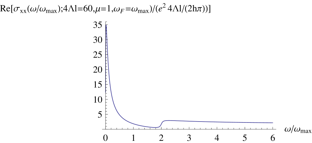
Figure 1: The conductivity for the entire frequency

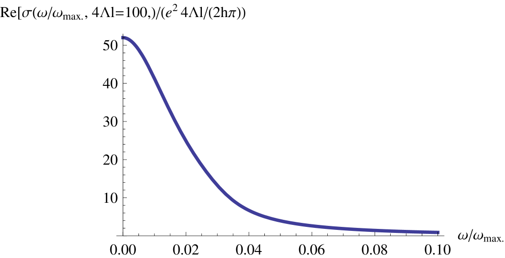
Figure 2: The conductivity at low frequencies

References

(1) B.A,Volkov and O.A.Pankratov Jetp Lett. 612015 (1988)
(2) C.L.Kane and E.J. Mele Phys.Rev.Lett.75,146802(2005)
(3) Xiao-Liang Qi and Shou-Cheng-Zhang Rev.Of Modern Physics 831057(2011)
(4) D.Schmeltzer Phys.Rev.B 73165301(2006) and Advances in Condensed Matter and Material Research Editors Hans Geelvinck and Sjaak Reyst volume 10 chapter , pages (2011).