NEAREST NEIGHBORS, PHASE TUBES AND GENERALIZED SYNCHRONIZATION

Abstract

In this paper we report for the first time on the necessity of the refinement of the concept of generalized chaotic synchronization. We show that the state vectors of the interacting chaotic systems being in the generalized synchronization regime are related with each other by the functional, but not the functional relation as it was assumed until now. We propose the phase tube approach explaining the essence of generalized synchronization and allowing the detection and the study of this regime in many relevant physical circumstances. The finding discussed in this Report gives a strong potential for new applications.

Chaotic synchronization is one of the fundamental phenomena, widely studied recently, having both theoretical and applied significance Boccaletti et al. (2002). One of the interesting and intricate types of the synchronous behavior of unidirectionally coupled chaotic oscillators is generalized synchronization (GS) Abarbanel et al. (1996); Hramov and Koronovskii (2005). This kind of synchronous behavior is said to mean the presence of a functional relation between the drive and response oscillator states Rulkov et al. (1995); Pyragas (1996) and has been observed in many systems both numerically Kocarev and Parlitz (1996); Zheng and Hu (2000); Hramov et al. (2005a) and experimentally Rulkov (1996); Rogers et al. (2004); Dmitriev et al. (2009), with many interesting features Zheng and Hu (2000); Hramov et al. (2008) and possible applications Terry and VanWiggeren (2001); Koronovskii et al. (2009) of this regime being revealed.

The definition of the GS regime generally accepted hitherto is the presence of a functional relation

$${\mathbf{y}(t)=\mathbf{F}[\mathbf{x}(t)]}$$ (1)

between the drive $\mathbf{x}(t)$ and response $\mathbf{y}(t)$ oscillator states Rulkov et al. (1995); Pyragas (1996). Having based on this definition the different techniques for detecting the presence of GS between chaotic oscillators had been proposed, such as the nearest neighbor method Rulkov et al. (1995); Parlitz et al. (1996), the auxiliary system approach Abarbanel et al. (1996) or the conditional Lyapunov exponent calculation Pyragas (1996), with the auxiliary system approach being generally the most easy, clear and powerful tool to study the GS regime in the model systems, whereas for the analysis of the observed experimental time series the nearest neighbor method, as a rule, is more applicable Dmitriev et al. (2009).

In this Report we report for the first time on the necessity of reconsidering and refining the existing concept of generalized chaotic synchronization. The main reason of this refinement is the following. Let $\mathbf{x}(t_{0})=\mathbf{x}_{0}$ and $\mathbf{y}(t_{0})=\mathbf{y}_{0}$ be the reference points belonging to the chaotic attractors of the drive and response oscillators being in the GS regime, respectively. For the neighbor point $\mathbf{x}(t_{i})=\mathbf{x}_{i}$ of the drive oscillator such that ${||\mathbf{x}_{i}-\mathbf{x}_{0}||<\varepsilon}$ its image $\mathbf{y}(t_{i})=\mathbf{y}_{i}$ in the response system is also close to the reference point $\mathbf{y}_{0}$ (see Rulkov et al. (1995) for detail), i.e., ${||\mathbf{y}_{i}-\mathbf{y}_{0}||<\delta(\varepsilon)}$. Having linearized Eq. (1), one obtains that

$$\mathbf{y}_{i}-\mathbf{y}_{0}=J\mathbf{F}[\mathbf{x}_{0}](\mathbf{x}_{i}-\mathbf{x}_{0}),$$ (2)

where $J$ is the Jacobian operator. Since the form of the functional relation $\mathbf{F}[\cdot]$ can not be found explicitly in most cases, Eq. (2) may be rewritten in the form

$$\delta\mathbf{y}_{i}=\mathbf{A}\delta\mathbf{x}_{i},$$ (3)

where $\mathbf{A}=J\mathbf{F}[\mathbf{x}_{0}]$ is the unknown matrix and ${\delta\mathbf{x}_{i}=\mathbf{x}_{i}-\mathbf{x}_{0}}$, ${\delta\mathbf{y}_{i}=\mathbf{y}_{i}-\mathbf{y}_{0}}$ are the vectors characterizing the deviation of the points under consideration $\mathbf{x}_{i}$, $\mathbf{y}_{i}$ from the reference points $\mathbf{x}_{0}$ and $\mathbf{y}_{0}$, respectively. Without the lack of generality we shall suppose below the identical dimension $m$ of the phase space of the drive and response systems.

Although the coefficients of the matrix $\mathbf{A}$ are unknown, the validity of Eq. (3) may be verified if there are $N>m$ nearest neighbors $\mathbf{x}_{i}$ of the reference point $\mathbf{x}_{0}$ and corresponding them vectors $\mathbf{y}_{i}$ of the response system. Having tested the presence of the generalized synchronization (e.g., with the help of the auxiliary system approach) we can pick out $m$ nearest neighbors $\mathbf{x}_{i}$ ($i=1,\dots,m$) and corresponding to them vectors $\mathbf{y}_{i}$ to determine the coefficients $a_{ij}$ of the matrix $\mathbf{A}$ with the help of Eq. (3). To reduce the influence of the inaccuracy we have to select such vectors $\mathbf{x}_{i}$ (and ${\delta\mathbf{x}_{i}=(\delta x_{i1},\dots,\delta x_{im})^{T}}$, respectively) from the whole set of $N$ vectors for which

$$|\det(\mathbf{X})|=\max,$$ (4)

where

$$\mathbf{X}=\left(\begin{array}[]{cccc}\delta x_{11}&\delta x_{12}&\ldots&\delta x_{1m}\\ \delta x_{21}&\delta x_{22}&\ldots&\delta x_{2m}\\ \vdots&\vdots&\ddots&\vdots\\ \delta x_{m1}&\delta x_{m2}&\ldots&\delta x_{mm}\\ \end{array}\right).$$ (5)

Having determined the matrix $\mathbf{A}$ we can now find the vectors $\delta\mathbf{z}_{i}$, (${i=m+1,\dots,N}$) as

$$\delta\mathbf{z}_{i}=\mathbf{A}\delta\mathbf{x}_{i},$$ (6)

and compare them with the vectors $\delta\mathbf{y}_{i}$ of the response system (or compare vectors ${\mathbf{z}_{i}=\mathbf{y}_{0}+\delta\mathbf{z}_{i}}$ with $\mathbf{y}_{i}$) to validate the correctness of Eq. (3).

Altought, at first sight, it seems that there are no fundamental causes due to which Eq. (3) may fail, in reality Eq. (3) is not correct. To illustrate this fact we have studied numerically the synchronous behavior of two coupled chaotic Rössler oscillators

$$\begin{array}[]{ll}\dot{x}_{d}=-\omega_{d}y_{d}-z_{d},&\dot{x}_{r}=-\omega_{r}y_{r}-z_{r}+\varepsilon(x_{d}-x_{r}),\\ \dot{y}_{d}=\omega_{d}x_{d}+ay_{d},&\dot{y}_{r}=\omega_{r}x_{r}+ay_{r},\\ \dot{z}_{d}=p+z_{d}(x_{d}-c),&\dot{z}_{r}=p+z_{r}(x_{r}-c),\\ \end{array}$$ (7)

where $\mathbf{x}=(x_{d},y_{d},z_{d})^{T}$ [$\mathbf{y}=(x_{r},y_{r},z_{r})^{T}$] are the cartesian coordinates of the drive [the response] oscillator, dots stand for temporal derivatives, and $\varepsilon$ is a parameter ruling the coupling strength. The other control parameters of Eq. (7) have been set to $a=0.15$, $p=0.2$, $c=10.0$, in analogy with our previous studies  Hramov and Koronovskii (2005); Hramov et al. (2005b). The $\omega_{r}$–parameter (representing the natural frequency of the response system) has been selected to be $\omega_{r}=0.95$; the analogous parameter for the drive system has been fixed to $\omega_{d}=0.99$. For such a choice of the parameter values the boundary of the generalized synchronization regime found with the help of the auxiliary system approach is around $\varepsilon_{GS}\approx 0.11$.

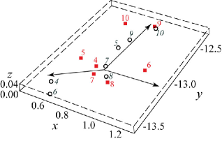
Figure 1: (Color online) The vectors $\mathbf{y}_{i}$ ($\blacksquare$) and $\mathbf{z}_{i}$ ($\circ$) of the response Rössler system (7) for $\varepsilon=0.3$. The numbers $i$ of the vectors are shown by the regular and italic fonts, respectively

Having chosen the reference point $\mathbf{x}_{0}$ of chaotic attractor of the drive oscillator randomly, one can find its nearest neighbors $\mathbf{x}_{i}$ ($i=1,\dots,N$) (and corresponding to them vectors $\mathbf{y}_{i}$ of the response system), select (according to Eqs. (4) and (5)) the vector basis $\mathbf{x}_{1-3}$ to determine the matrix $\mathbf{A}$ and check condition (3) with the help of Eq. (6) and the rest of vectors $\mathbf{x}_{i}$, $\mathbf{y}_{i}$, ($i=4,\dots,N$).

In Fig. 1 the vectors $\mathbf{z}_{i}$ ($i=4,\dots,10$) obtained with the help of Eq. (6) as well as the vectors $\mathbf{y}_{i}$ of the response system are shown for the coupling strength $\varepsilon=0.3$. The value of the coupling strength exceeds greatly the threshold $\varepsilon_{GS}$ of the generalized synchronization, the GS regime demonstrate great stability, and, as a consequence, Eq. (3) is expected to be correct. However, contrary to expectations, the vectors $\mathbf{z}_{i}$ and $\mathbf{y}_{i}$ differ from each other sufficiently testifying that Eq. (3) fails. As a matter of fact, the failure of Eq. (3) is also observed for other reference points of the drive Rössler oscillator as well as for other chaotic dynamical systems (e.g., Lorenz oscillators). Since Eq. (3) is just the linearization of Eq. (1), the failure of Eq. (3) is the evidence of the incorrectness of Eq. (1) being the main definition of the generalized synchronization concept. At the same time, plenty of results obtained hitherto are in the very good agreement with the generally accepted concept of GS. It means that the concept proposed by N. Rulkov et al. Rulkov et al. (1995) works in some circumstances, but, in general, must be refined.

The core idea of this correction is the following. The state of the response system $\mathbf{y}(t)$ depends not only on the state of the drive oscillator $\mathbf{x}(t)$ at the moment of time $t$, but on the history of the evolution of the drive system during time interval $(t-\tau,t]$ as well. Indeed, according to the concept of GS, synchronization means that the response oscillator $\mathbf{y}(t)$ comes to the state defined uniquely by the drive system, with the convergence time $\tau$ being connected with the largest conditional Lyapunov exponent $\lambda_{1}^{r}$, i.e. $\tau\sim 1/|\lambda_{1}^{r}|$. In other words, $\mathbf{F}[\cdot]$ in Eq. (1) must be considered as a functional, but not a functional relation. Obviously, in this case Eq. (3) obtained under assumptions that $\mathbf{F}[\cdot]$ is the functional relation is not satisfied as it has been shown above (see Fig. 1).

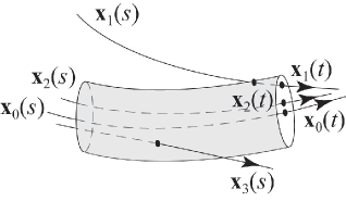
Figure 2: The schematic representation of the nearest vectors $\mathbf{x}_{i}(t)$, the phase trajectories $\mathbf{x}_{i}(s)$ and the phase tube $\mathbb{T}_{\tau}(t)$

Considering $\mathbf{F}[\cdot]$ as the functional, one have to replace Eq. (2) by

$$\delta\mathbf{y}_{i}(t)=\int\limits_{t-\tau}^{t}J\mathbf{F}[\mathbf{x}_{0}(s)]\delta\mathbf{x}_{i}(s)\,ds.$$ (8)

Having supposed that the deviation $\delta\mathbf{x}_{i}(s)$ from the reference trajectory $\mathbf{x}_{0}(s)$ (${t-\tau<s\leq t}$) is small, in view of the linearity one can write

$$\delta\mathbf{x}_{i}(s)=\mathbf{B}(s)\delta\mathbf{x}_{i}(t),\quad t-\tau<s<t,$$ (9)

(where $\mathbf{B}(s)$ is the matrix with the time-dependent coefficients) that results in

$$\delta\mathbf{y}_{i}(t)=\int\limits_{t-\tau}^{t}J\mathbf{F}[\mathbf{x}_{0}(s)]\mathbf{B}(s)\delta\mathbf{x}_{i}(t)\,ds.$$ (10)

and, as a consequence, in

$$\delta\mathbf{y}_{i}(t)=\mathbf{C}(t)\delta\mathbf{x}_{i}(t),$$ (11)

where $\mathbf{C}(t)$ is the square $(m\times m)$-matrix defined as

$$\mathbf{C}(t)=\int\limits_{t-\tau}^{t}J\mathbf{F}[\mathbf{x}_{i}(s)]\mathbf{B}(s)\,ds.$$ (12)

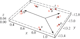
Figure 3: (Color online) The vectors $\mathbf{y}_{i}$ ($\blacksquare$) and $\mathbf{z}_{i}$ ($\circ$) of the response Rössler system (7) for $\varepsilon=0.3$, the length of the phase tube is $\tau=100$. The numbers $i$ of the vectors are shown by the regular and italic fonts, respectively

So, Eq. (11) coincides formally with Eq. (3) and, therefore, it may be also validated by the calculations of vectors $\mathbf{z}_{i}$ in the same way as it has been done for Eq. (3). At the same time, Eq. (3) has been obtained under assumptions that the vectors $\mathbf{x}_{0}(t)$ and $\mathbf{x}_{i}(t)$ are close to each other, whereas Eq. (11) has been obtained for more stricter restriction requiring the nearness of the trajectories $\mathbf{x}_{0}(s)$ and $\mathbf{x}_{i}(s)$ during the time interval ${t-\tau<s\leq t}$. Since for the chaotic systems the phase trajectories can converge in one direction of the phase space and diverge in another one, the neighbor vectors $\mathbf{x}_{0}(t)$ and $\mathbf{x}_{i}(t)$ may be characterized by the very distinct phase trajectories $\mathbf{x}_{0}(s)$ and $\mathbf{x}_{i}(s)$ for ${t-\tau<s\leq t}$. The schematic representation of such a situation is given in Fig. 2. Although the vectors $\mathbf{x}_{1}(t)$ and $\mathbf{x}_{2}(t)$ are close to the reference point $\mathbf{x}_{0}(t)$, only the vector $\mathbf{x}_{2}(t)$ obeys Eq. (11) due to the nearness of the phase trajectories $\mathbf{x}_{0}(s)$ and $\mathbf{x}_{2}(s)$, whereas for the vector $\mathbf{x}_{1}(t)$ Eq. (11) fails, since the phase trajectory $\mathbf{x}_{1}(s)$ is not close to the reference one $\mathbf{x}_{0}(s)$ during the whole time interval ${t-\tau<s\leq t}$. Therefore, to verify Eq. (11) we have to consider not all vectors $\mathbf{x}_{i}(t)$ being nearest to the reference point $\mathbf{x}_{0}(t)$, but only vectors which are characterized by the phase trajectories $\mathbf{x}_{i}(s)$ being close to the reference one $\mathbf{x}_{0}(s)$. Having based on the idea of phase space strands Kennel and Abarbanel (2002); Carroll (2011), to eliminate the ineligible vectors (like $\mathbf{x}_{1}(t)$ in Fig. 2) we introduce into consideration the phase tube

$$\mathbb{T}_{\tau}(t)=\{\mathbf{x}:\left.\left|x_{0j}(s)-x_{j}\right|<d_{j}\right|_{j=1}^{m},s\in[t-\tau;t]\}$$ (13)

and take into account only vectors whose phase trajectories pass through this phase tube (like $\mathbf{x}_{2}(t)$ in Fig. 2).

The result of this examination for Rössler systems (7) with the same set of the control parameter values and the coupling strength as before is given in Fig. 3, the length of the phase tube is $\tau=100$. One can see that the calculated vectors $\mathbf{z}_{i}(t)$ are in the excellent agreement with the vectors $\mathbf{y}_{i}(t)$ of the response Rössler system that confirms both the correctness of Eq. (11) and, as a consequence, the statement that $\mathbf{F}[\cdot]$ is the functional, but not the functional relation.

With the increase of the coupling strength between chaotic oscillators the absolute value of the largest conditional Lyapunov exponent $\lambda_{1}^{r}$ grows, whereas the time interval $\tau$ (the length of the phase tube $\mathbb{T}_{\tau}(t)$) decreases. Finally, in the lag synchronization (LS) and complete synchronization (CS) regimes the value of $\tau$ tends to be zero. Therefore, in the LS and CS regimes Eq. (3) is satisfied for all neighbor vectors $\mathbf{x}_{i}(t)$ without any additional requirements concerning the phase trajectory nearness. In other words, the state vectors of any chaotic systems being in the GS regime (but not in the LS or CS regime) are connected with each other with the functional, whereas in the LS and CS regimes (which are the strong form of GS) they are related with each other by the functional relation.

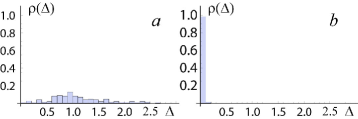
Figure 4: The histograms of the normalized difference $\Delta=||\delta\mathbf{y}_{i}(t)-\delta\mathbf{z}_{i}(t))||/||\delta\mathbf{y}_{i}(t)||$ for (a) the asynchronous dynamics, $\varepsilon=0.06$ and (b) the generalized synchronization regime, $\varepsilon=0.3$. The histograms have been obtained for the response Rössler system (7), the length of the phase tube is $\tau=100$

Though the phase tube approach has been here applied to the model systems, we expect that it can be used in many other relevant circumstances. Since the statistics for the difference between $\delta\mathbf{y}_{i}(t)$ and $\delta\mathbf{z}_{i}(t)$ vectors are radically different for the synchronous and asynchronous motion (see Fig. 4), the important feature of this approach is the possibility to consider the relation between vectors (11) for the analysis of the registered experimental data (vector or scalar, using the Takens approach Takens (1981)) when the other classical methods of GS detection are inaccurate or unapplicable. Moreover, the proposed approach may be used as the method to detect the GS regime, including the case when the chaotic oscillators are coupled mutually, since all arguments given above are also applicable for the case of the bidirectional coupling.

To prove the generality of our findings we have also studied numerically two mutually coupled generators with tunnel diodes . In the dimensionless form the dynamics of such generators is described by the equations Rosenblum et al. (1997); Koronovskii et al. (2007)

$$\begin{array}[]{l}\dot{x}_{1,2}=\omega^{2}_{1,2}[h(x_{1,2}-\varepsilon(y_{2,1}-y_{1,2}))+y_{1,2}-z_{1,2}],\\ \dot{y}_{1,2}=-x_{1,2}+\varepsilon(y_{2,1}-y_{1,2}),\\ \mu\dot{z}_{1,2}=x_{1,2}-f(z_{1,2}),\end{array}$$ (14)

where ${f(\xi)=-\xi+0.002\mathrm{sh}(5\xi-7.5)+2.9}$ is the dimensionless characteristics of nonlinear converter, ${h=0.2}$, ${\mu=0.1}$, ${\omega_{1}=1.09}$, ${\omega_{2}=1.02}$ are the control parameter values, $\varepsilon$ is the coupling parameter strength. The indexes “1” and “2” correspond to the first and second coupled systems, respectively. For such values of the control parameters the threshold of the generalized synchronization regime determined by the moment of the transition of the second positive Lyapunov exponent in the field of the negative values Moskalenko et al. (2010); Koronovskii et al. (2011) is around $\varepsilon_{GS}\approx 0.08$.

As in the case of Rössler systems considered above we have chosen the reference point $\mathbf{x}_{0}$ of chaotic attractor of the first oscillator randomly and analyze the behavior of its nearest neighbors $\mathbf{x}_{i}$ ($i=1,\dots,N$) and corresponding to them vectors $\mathbf{y}_{i}$ and $\mathbf{z}_{i}$. The choice of the vector basis $\mathbf{x}_{1-3}$ has been performed in the same way as in the case considered above.

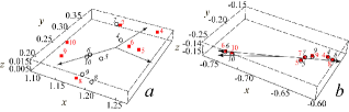
Figure 5: (Color online) The vectors $\mathbf{y}_{i}$ ($\blacksquare$) and $\mathbf{z}_{i}$ ($\circ$) of the second generator with tunnel diode (14) for $\varepsilon=0.15$. The numbers $i$ of the vectors are shown by the regular and italic fonts, respectively. (a) All neighbor vectors are used; (b) only vectors whose phase trajectories pass through the phase tube with length $\tau=110$ are used

In Fig. 5 the vectors $\mathbf{y}_{i}$ ($\blacksquare$) and $\mathbf{z}_{i}$ ($\circ$) of the second generator with tunnel diode (14) for the coupling parameter strength $\varepsilon=0.15$ exceeding greatly the threshold value of the generalized synchronization regime onset $\varepsilon_{GS}$ are shown. Fig. 5,a corresponds to the case when all neighbor vectors are used whereas in Fig. 5,b only vectors whose phase trajectories pass through the phase tube with length $\tau=110$ are used. It is clearly seen that in the first case the vectors $\mathbf{z}_{i}$ and $\mathbf{y}_{i}$ differ from each other sufficiently testifying the failure of the presence of the functional relation between the interacted system states. But, conversely, for the phase tube with the length $\tau=110$ (Fig. 5,b) the calculated vectors $\mathbf{z}_{i}(t)$ are in the excellent agreement with the vectors $\mathbf{y}_{i}(t)$ of the second generator that confirms the results obtained above for unidirectionally coupled Rössler systems. So, in the systems with a mutual type of coupling the vector states of the interacting systems are related with each other by the functional.

In conclusion, we have reported that the concept of generalized synchronization (except for the LS and CS regimes) needs refining, since the state vectors of the interacting chaotic systems are related with each other by the functional, but not the functional relation as it was assumed until now. Although in the Report the systems with a small number of degrees of freedom have been considered, the developed formalism can be also extended to the systems with the infinite-dimensional phase space . Fortunately, this modification of the generalized synchronization concept does not discard the majority of the obtained hitherto results concerning GS. At the same time, this refinement has a fundamental significance from the point of view of the understanding of the core mechanisms of the considered phenomena and is supposed to give a strong potential for new approaches and applications dealing with the nonlinear systems.

References

- Boccaletti et al. (2002) S. Boccaletti, J. Kurths, G. V. Osipov, D. L. Valladares, and C. S. Zhou, Physics Reports 366, 1 (2002).
- Abarbanel et al. (1996) H. D. Abarbanel, N. F. Rulkov, and M. M. Sushchik, Phys. Rev. E 53, 4528 (1996).
- Hramov and Koronovskii (2005) A. E. Hramov and A. A. Koronovskii, Phys. Rev. E 71, 067201 (2005).
- Rulkov et al. (1995) N. F. Rulkov, M. M. Sushchik, L. S. Tsimring, and H. D. Abarbanel, Phys. Rev. E 51, 980 (1995).
- Pyragas (1996) K. Pyragas, Phys. Rev. E 54, R4508 (1996).
- Kocarev and Parlitz (1996) L. Kocarev and U. Parlitz, Phys. Rev. Lett. 76, 1816 (1996).
- Zheng and Hu (2000) Z. Zheng and G. Hu, Phys. Rev. E 62, 7882 (2000).
- Hramov et al. (2005a) A. E. Hramov, A. A. Koronovskii, and P. V. Popov, Phys. Rev. E 72, 037201 (2005a).
- Rulkov (1996) N. F. Rulkov, Chaos 6, 262 (1996).
- Rogers et al. (2004) E. A. Rogers, R. Kalra, R. D. Schroll, A. Uchida, D. P. Lathrop, and R. Roy, Phys.Rev.Lett. 93, 084101 (2004).
- Dmitriev et al. (2009) B. S. Dmitriev, A. E. Hramov, A. A. Koronovskii, A. V. Starodubov, D. I. Trubetskov, and Y. D. Zharkov, Physical Review Letters 102, 074101 (2009).
- Hramov et al. (2008) A. E. Hramov, A. A. Koronovskii, and P. V. Popov, Phys. Rev. E 77, 036215 (2008).
- Terry and VanWiggeren (2001) J. R. Terry and G. D. VanWiggeren, Chaos, Solitons and Fractals 12, 145 (2001).
- Koronovskii et al. (2009) A. A. Koronovskii, O. I. Moskalenko, and A. E. Hramov, Physics-Uspekhi 52, 1213 (2009).
- Parlitz et al. (1996) U. Parlitz, L. Junge, W. Lauterborn, and L. Kocarev, Phys. Rev. E 54, 2115 (1996).
- Hramov et al. (2005b) A. E. Hramov, A. A. Koronovskii, and O. I. Moskalenko, Europhysics Letters 72, 901 (2005b).
- Kennel and Abarbanel (2002) M. Kennel and H. D. Abarbanel, Phys. Rev. E 66, 026209 (2002).
- Carroll (2011) T. L. Carroll, Chaos 21, 023128 (2011).
- Takens (1981) F. Takens, in Lectures Notes in Mathematics, edited by D. Rand and L.-S. Young (N. Y.: Springler–Verlag, 1981), p. 366.
- Rosenblum et al. (1997) M. G. Rosenblum, A. S. Pikovsky, and J. Kurths, IEEE Transactions on Circuits and Systems I 44, 874 (1997).
- Koronovskii et al. (2007) A. A. Koronovskii, M. K. Kurovskaya, O. I. Moskalenko, and A. E. Hramov, Technical Physics 52, 19 (2007).
- Moskalenko et al. (2010) O. I. Moskalenko, A. A. Koronovskii, A. E. Hramov, and S. A. Shurygina, Proceedings of 18th IEEE Workshop on Nonlinear Dynamics of Electronic Systems pp. 70–73 (2010).
- Koronovskii et al. (2011) A. A. Koronovskii, O. I. Moskalenko, V. A. Maksimenko, and A. E. Hramov, Technical Physics Letters 37, 611 (2011).