Finite volume effects and quark mass dependence of the $N(1535)$ and $N(1650)$

Abstract

For resonances decaying in a finite volume, the simple identification of state and eigenvalue is lost. The extraction of the scattering amplitude is a major challenge as we demonstrate by extrapolating the physical $S_{11}$ amplitude of pion-nucleon scattering to the finite volume and unphysical quark masses, using a unitarized chiral framework including all next-to-leading order contact terms. We show that the pole movement of the resonances $N(1535)1/2^{-}$ and $N(1650)1/2^{-}$ with varying quark masses is non-trivial. In addition, there are several strongly coupled $S$-wave thresholds that induce a similar avoided level crossing as narrow resonances. The level spectrum is predicted for two typical lattice setups, and ways to extract the amplitude from upcoming lattice data are discussed.

1 Introduction

Pion-nucleon scattering has traditionally been the premier reaction to study the resonance excitations of the nucleon. In particular, in the $S_{11}$ partial wave one finds two close-by resonances at 1535 and 1650 MeV, which overlap within their widths of about 100 MeV. It was pointed out early in the framework of unitarized coupled-channel chiral perturbation theory [1] that the $N(1535)1/2^{-}$ might not be a three-quark resonance, but is rather generated by strong channel couplings with a dominant $K\Sigma-K\Lambda$ component in its wave function. This analysis was extended in Ref. [2], where within certain approximations the effects of 3-body $\pi\pi N$ channels were also included. Further progress was made in Ref. [3], where the $S_{11}$ phase shift was fitted from threshold to about $W=\sqrt{s}\simeq 2\,$GeV together with cross section data for $\pi^{-}p\to\eta n$ and $\pi^{-}p\to K^{0}\Lambda$ in the respective threshold regions. More recently, it was pointed out in a state-of-the-art unitary meson-exchange model [4] that there is indeed strong resonance interference between the two $S_{11}$ resonances, as each of these resonances provides an energy-dependent background in the region of the other. In Ref. [5] the coupled-channel problem in the $J^{P}=1/2^{-}$ (with $J$ the spin and $P$ the parity) sector was addressed, for the first time, using the full off-shell Bethe-Salpeter equation and all contact terms of the leading and next-to-leading order (NLO) in the chiral expansion of the meson-baryon interaction. Remarkably, not only the $N(1535)1/2^{-}$ emerged from the meson-baryon dynamics, but also the $N(1650)1/2^{-}$ could be predicted without being included in the fit.

Another source of experimental information on the $J^{P}=1/2^{-}$ and other resonances is provided by the dedicated baryon resonance programs at ELSA, MAMI and Jefferson Lab [6, 7]. On the theoretical side, the concept of dynamical resonance generation has been investigated in [8, 9, 10, 11, 12] comparing with the extracted multipoles and helicity amplitudes from the SAID and MAID analyses [13, 14, 15, 16]. Of particular interest is the gauge invariant scheme developed for the full off-shell Bethe-Salpeter equation [17] that has been applied to pion and eta photoproduction [8, 9].

Finally, lattice gauge simulations have rapidly evolved and the spectrum of excited baryons starts to become accessible, in particular also for the $J^{P}=1/2^{-}$ sector [18, 19, 20, 21, 22, 23]. As quark masses come closer to the physical limit, finite volume effects dominate the lattice spectrum. Further, as resonances start to decay their signal on the lattice is lost. Still, Lüscher has shown how to model-independently extract phase shifts from lattice levels [24, 25] (see also [26]). For example, Lang and Verduci recently provided such levels above threshold, for the first time in the $J^{P}=1/2^{-}$ sector [18]. Lüscher’s method can be combined with effective field theory to study baryonic resonances and their width in the finite volume [27, 28]. The extension to coupled channels has been pioneered in Ref. [29] (see also [30]) and further applied to excited mesons [31, 32, 33]. For a different approach, see Ref. [34].

Using these techniques in combination with the unitarized chiral approach of Ref. [5], we predict in this Letter the finite-volume level spectrum of the $S_{11}$ partial wave, extrapolated to unphysical quark masses. In addition, we test the hypothesis that the hidden-strangeness $KY$ channels provide the crucial dynamics for the resonance generation by applying twisted boundary conditions for the strange quark. As we will show, the interplay between thresholds and resonances is very intricate and need to be accounted for in any extraction of resonance properties in this partial wave (and for other processes that exhibit similar properties).

2 Framework

2.1 Pion-nucleon scattering in the infinite volume

In the present work we rely on the model for the description of meson-baryon scattering in the first and second resonance region as developed in Ref. [5]. There, the Bethe-Salpeter equation has been solved including the full off-shell dependence of the chiral potential. The latter has been chosen to consist of all local terms of first and second chiral order, omitting, however, the one–baryon exchange graphs from the beginning. Including two-body channels with quantum numbers of the pion-nucleon system, the model describes the $S_{11}$ partial wave rather well up to quite high energies, i.e. $W\lesssim 1800$ MeV. In particular, this framework allows for a dynamical generation of both negative-parity nucleonic resonances, the $N(1535)1/2^{-}$ and $N(1650)1/2^{-}$.

For two-particle scattering, we denote the in- and out-going meson momenta by $q_{1}$ and $q_{2}$, respectively. The overall four-momentum is $p=q_{1}+p_{1}=q_{2}+p_{2}$, where $p_{1}$ and $p_{2}$ are the momenta of in- and outgoing baryon, respectively. For the unitary meson-baryon scattering amplitude $T(q_{2},q_{1};p)$ and the potential $V(q_{2},q_{1};p)$, the Bethe-Salpeter integral equation reads in $d$ dimensions

$$T({q}_{2},{q}_{1};p) =V(q_{2},q_{1};p)$$ (1)

$$+i\int\frac{d^{d}\ell}{(2\pi)^{d}}\frac{V({q}_{2},{\ell};p)\,(\not{p}-\not{\ell}+m)\,T({\ell},{q}_{1};p)}{({\ell^{2}-M^{2}+i\epsilon})((p-\ell)^{2}-m^{2}+i\epsilon)}~{},$$

where $m$ and $M$ denote the mass of baryon and meson, respectively. This equation has to be understood as a matrix equation in channel space, and the channel space is constructed from a certain number of the allowed combinations of one ground-state octet meson and one ground-state octet baryon. For isospin $I=1/2$ and strangeness $S=0$ the channels are $\pi N$, $\eta N$, $K\Lambda$, and $K\Sigma$. The propagator is diagonal in channel space.

By maintaining the full off-shell dependence, the identification of every term of Eq. (1) with Feynman diagrams is ensured, which for instance allows for the construction of a gauge invariant photoproduction amplitude [8] in a very natural way. However, in a finite volume the Passarino-Veltmann reduction utilized for the solution of Eq. (1) in Refs. [5, 8] is a-priori no longer applicable. To overcome this complication we set all tadpole integrals to zero in this solution, which puts for instance the potential $V$ on the two-particle mass shell. This simplifies Eq. (1) to the following algebraic equation

$$T^{\rm on}=V^{\rm on}+V^{\rm on}GT^{\rm on}~{},$$ (2)

where all elements are again matrices in channel space and the remaining loop function $G$ reads

$$G :=i\mathop{\int}\frac{d^{d}\ell}{(2\pi)^{d}}\frac{\not{p}-\not{\ell}+m}{(\ell^{2}-M^{2}+i\epsilon)((p-\ell)^{2}-m^{2}+i\epsilon)}$$

$$~{}=\Big{(}\not{p}\frac{p^{2}-M^{2}+m^{2}}{2p^{2}}+m\Big{)}\,I_{MB}~{}.$$ (3)

Here $I_{MB}$ denotes the scalar one-meson-one-baryon loop integral. The factor in parenthesis in the second line yields

$$(\ldots)=2m+\boldsymbol{\gamma}\cdot\boldsymbol{p}_{\rm cms}~{},$$ (4)

where $\boldsymbol{p}_{\rm cms}$ denotes the baryon three-momentum in the c.m. frame. This demonstrates the difference to another on-shell scheme that is widely used in the literature (see, e.g., Refs. [2, 10]) in which the term $\boldsymbol{\gamma}\cdot\boldsymbol{p}_{{\rm cms}}$ is omitted.

The renormalization of loop divergences in non-perturbative frameworks is known to be complicated. Relying on the arguments given in Refs. [5, 8], we utilize dimensional regularization, applying the usual $\overline{\rm MS}$ scheme. The finite part of scalar loop integral reads in four space-time dimensions

$$I^{\rm fin}_{MB}\overset{d=4}{=}\frac{1}{16\pi^{2}}\left[-1+2\log\left(\frac{m}{\mu}\right)+\frac{M^{2}-m^{2}+s}{s}\log\left(\frac{M}{m}\right)\right.-$$

$$-\left.\frac{4p_{{\rm cms}}}{\sqrt{s}}\,\mathrm{arctanh}\left(\frac{2p_{{\rm cms}}\sqrt{s}}{(m+M)^{2}-s}\right)\right]~{},$$ (5)

where $\mu$ is the regularization scale and $p_{{\rm cms}}$ is the modulus of the center-of-mass three momentum, expressed in terms of the Källén function as $p_{{\rm cms}}=\lambda^{1/2}(s,m^{2},M^{2})/(2\sqrt{s})$. The $\mu$–dependence would be canceled by the corresponding scale dependence of the higher-order counter terms. Dealing with a non-perturbative framework with only a finite number of terms being iterated, such a cancellation is not possible, which is the reason why in most comparable approaches this scale is used as a free parameter. Here we fix it to the values (in GeV) found in fitting strategy II of Ref. [8], namely $\log(\mu_{\pi}/(1\text{GeV}))=-0.368$, $\log(\mu_{\eta}/(1\text{ GeV}))=0.056$ and $\log(\mu_{K}/(1\text{ GeV}))=0.210$.

The following hadron masses and decay constants are used (all in MeV):

$m_{N}=939$,	$M_{\pi}=138$,	$F_{\pi}=92.4$,
$m_{\Sigma}=1195$,	$M_{K}=495$,	$F_{K}=113.0$,
$m_{\Lambda}=1115.7$,	$M_{\eta}=547$,	$F_{\eta}=1.3F_{\pi}$.

The free parameters of the model are given by 14 low-energy constants of the next-to-leading chiral order, appearing in the potential $V$. All 14 parameters are adjusted here to reproduce the current SAID solution [14] for the real and imaginary part of the $S_{11}$ partial wave in the energy region ${1080\leq W\leq 1800}$ MeV. The errors are assigned as described in Ref. [5], namely $\Delta S_{11}=0.005$ for $W\leq 1280$ MeV and $\Delta S_{11}=0.030$ for higher energies.

Figure 1: The $S_{11}$ amplitude. Upper panel: Best fit of the model to the energy independent solution of the PWA by the SAID group [14]. Red (solid) and blue (dashed) lines represent the real and imaginary part of our solution, respectively, whereas the vertical dashed lines correspond to the two-particle thresholds. Lower left panel: Riemann sheet connected to the physical axis between the $\eta N$ and the $K\Lambda$ threshold. Right: sheet connected to the physical axis between $K\Lambda$ and $K\Sigma$ threshold. See text for the labeling of the poles.

The best fit of our model is presented in Fig. 1. The fitted parameters are (all $b_{i}$ in GeV^-1):

$$b_{1} =-0.765, b_{6} =-1.043, b_{11} =-1.220,$$

$$b_{2} =+0.924, b_{7} =+5.919, b_{0} =-1.186,$$

$$b_{3} =-2.610, b_{8} =+0.732, b_{D} =+1.173,$$

$$b_{4} =+0.892, b_{9} =-1.304, b_{F} =-0.624,$$

$$b_{5} =+0.023, b_{10} =+1.401.$$

Note that these fit parameters differ from those in Ref. [8] due to the on-shell approximation performed here.

At the pion-nucleon threshold we extract the scattering length to be $a_{\pi N}^{1/2}=1.13$ GeV^-1, which is somewhat smaller than in the earlier analysis of Ref. [8], i.e. $a_{\pi N}^{1/2}=1.22$ GeV^-1. The analytic structure of the amplitude is shown in the two lower panels of Fig. 1 for two sheets. The left panel shows the Riemann sheet that is directly connected to the physical axis between the $\eta N$ and the $K\Lambda$ threshold as indicated with the thick horizontal bar. Performing the analytic continuation of the scattering amplitude we locate the poles on this sheet at

$$W_{N(1535)} =(1487-i\,\,\,\,84)\text{ MeV},$$

$$W_{N^{\prime}~{}~{}~{}~{}~{}~{}} =(1675-i\,103)\text{ MeV (hidden)},$$ (6)

where one pole can obviously be identified with the $N(1535)1/2^{-}$ resonance and another one ($N^{\prime}$) is hidden behind the $K\Lambda$ threshold. Apart from poles, we find on this sheet also a zero at $W_{0}=(1592-i\,62)$ MeV. The SAID group found a zero at $W_{0}=(1578-i\,38)$ MeV [35]. On the sheet connected to the physical axis between the $K\Lambda$ and the $K\Sigma$ threshold (right panel), we find the pole of the $N(1650)1/2^{-}$ at

$$W_{N(1650)}=(1658-i\,94)\text{ MeV}.$$ (7)

Again, for the more precise determination of the pole positions and scattering lengths, using the full off-shell solution of the Bethe-Salpeter equation, we refer the reader to original calculations [5, 8]. In any case, the values found here are well within the limits quoted by the Particle Data Group [36].

We do not perform an error analysis on the extracted low energy constants or amplitudes as performed in Ref. [8]. The error we are interested in here is the one expected for the finite volume spectrum extrapolated to unphysical masses. This will be discussed below.

2.2 Discretization

In the infinite volume all meson-baryon momenta are permitted while in a cubic volume of side length $L$ only momenta

$$\boldsymbol{q}=\frac{2\pi}{L}\,\boldsymbol{n},\quad\quad\boldsymbol{n}\in\mathds{Z}^{3}$$ (8)

are allowed due to the imposed periodic boundary conditions. In particular, the momentum integration over intermediate meson-baryon states of the propagator function $I_{MB}$ in Eq. (3) is replaced by a sum according to

$$\int\frac{d^{3}\boldsymbol{q}}{(2\pi)^{3}}\,f(|\boldsymbol{q}\,|)\to\frac{1}{L^{3}}\sum_{\boldsymbol{n}}\,f(|\boldsymbol{q}|)\ .$$ (9)

To obtain the three-momentum part of the integration of $I_{MB}$ we integrate over the zero component with external momentum $p=(\sqrt{s},\boldsymbol{0})$,

$$I_{MB} =\int\frac{d^{4}q}{(2\pi)^{4}}\,\frac{i}{(p-q)^{2}-m+i\epsilon}\frac{1}{q^{2}-M^{2}+i\epsilon}$$

$$=\int\frac{d^{3}\boldsymbol{q}}{(2\pi)^{3}}\,f(|\boldsymbol{q}|)\ ,$$

$$f(|\boldsymbol{q}|)=\frac{1}{2\omega_{m}(\boldsymbol{q})\,\omega_{M}(\boldsymbol{q})}\,\frac{\omega_{m}(\boldsymbol{q})+\omega_{M}(\boldsymbol{q})}{s-\left[\omega_{m}(\boldsymbol{q})+\omega_{M}(\boldsymbol{q})\right]^{2}+i\epsilon}\ ,$$ (10)

where $\omega_{m}(\boldsymbol{q})=\sqrt{m^{2}+\boldsymbol{q}^{2}}$ and $\omega_{M}(\boldsymbol{q})=\sqrt{M^{2}+\boldsymbol{q}^{2}}$. Using Eq. (9), this expression yields the finite-volume propagator $\tilde{I}_{MB}$ that still requires a regularization. We can proceed similar to Ref. [32] to express $\tilde{I}_{MB}$ as

$$\tilde{I}_{MB}=I_{MB}+\Delta I_{MB}$$ (11)

with the advantage that the regularization of the infinite volume is manifestly contained in $I_{MB}$, while $\Delta I_{MB}$ is the finite difference between the infinite-volume and the finite-volume expression, given above threshold by

$$\Delta I_{MB}=\tilde{I}_{MB}(s)-I_{MB}(s)=\biggl{\{}\frac{1}{L^{3}}\sum_{\boldsymbol{q}}^{|\boldsymbol{q}|<q_{\rm max}}-\int\limits^{|\boldsymbol{q}|<q_{\rm max}}\frac{d^{3}\boldsymbol{q}}{(2\pi)^{3}}\,\biggr{\}}\\ \times\,\frac{1}{2\sqrt{s}}\frac{1}{p_{{\rm cms}}^{2}-\boldsymbol{q}^{2}+i\epsilon}+\cdots=\frac{1}{2\sqrt{s}}\,\frac{1}{L^{3}}\sum_{\boldsymbol{q}}^{|\boldsymbol{q}|<q_{\rm max}}\frac{1}{p_{{\rm cms}}^{2}-\boldsymbol{q}^{2}}\\ +\frac{1}{4\pi^{2}\sqrt{s}}\,\left(q_{\rm max}+\frac{p_{{\rm cms}}}{2}\log\frac{q_{\rm max}-p_{{\rm cms}}}{q_{\rm max}+p_{{\rm cms}}}\right)+\frac{ip_{{\rm cms}}}{8\pi\,\sqrt{s}}+\cdots\,,$$ (12)

where the ellipses stand for the exponentially suppressed terms. Below threshold, the last term on the r.h.s. becomes real as the analytic continuation of $p_{{\rm cms}}$ becomes imaginary.

Moreover, as seen from Eq. (12), one may in fact remove here the cutoff, sending $q_{\rm max}\to\infty$. Indeed, one should obviously take a $q_{\rm max}$ such that $p_{{\rm cms}}^{2}<q_{\rm max}^{2}$ in the whole region of interest to us. If we sum and integrate from $q_{\rm max}$ to $q_{\rm max}^{\prime}$, with $q_{\rm max}^{\prime}>q_{\rm max}$, the denominator $p_{{\rm cms}}^{2}-\boldsymbol{q}^{2}$ is not singular and, according to the regular summation theorem, only exponentially suppressed corrections may arise. Finally, noting that (see, e.g. Ref. [37])

$$\lim_{q_{\rm max}\to\infty}\biggl{\{}\frac{1}{L^{3}}\sum_{\boldsymbol{q}}^{|\boldsymbol{q}|<q_{\rm max}}\frac{1}{p_{{\rm cms}}^{2}-\boldsymbol{q}^{2}}-\frac{q_{\rm max}}{2\pi^{2}}\biggr{\}}=-\displaystyle\frac{{\cal Z}_{00}(1,\hat{\boldsymbol{p}}^{2})}{2\pi^{3/2}L}\,,$$ (13)

where $\hat{\boldsymbol{p}}=({\boldsymbol{p}L})/({2\pi})$ and ${\cal Z}_{00}$ stands for the Lüscher zeta-function [24, 25], we can identify $\tilde{I}_{MB}$ with the Lüscher function up to exponentially suppressed terms

$$\tilde{I}_{MB}\simeq I_{MB}-\frac{1}{4\pi^{3/2}\sqrt{s}L}\,{\cal Z}_{00}(1;\hat{\boldsymbol{p}}^{2})+i\,\frac{p_{{\rm cms}}}{8\pi\sqrt{s}}\ .$$ (14)

In practical terms, we obtain the finite volume propagator by substituting the imaginary part of the infinite volume propagator according to

$$\tilde{I}_{MB}={\rm Re}\,I^{\rm fin}_{MB}+\delta I_{MB},\quad\delta I_{MB}=\tilde{G}_{S}-{\rm Re}\,G_{S}$$ (15)

with $\tilde{G}_{S}$ and $G_{S}$ defined in Eq. (15) of Ref. [32] and $I_{MB}^{\rm fin}$ from Eq. (5). The summation over lattice momenta can be simplified by the use of the $\theta$–series [38]. It should also be stressed that up to exponentially suppressed terms this is equivalent to the $K$-matrix formalism developed in Ref. [31]. A very similar approach to evaluate the discretized version of dimensionally regularized loops has been developed in Ref. [39].

Hybrid boundary conditions were introduced in Ref. [40] to distinguish scattering states from tightly bound quark-antiquark systems. Similarly, as proposed in Refs. [31, 32], twisted boundary conditions provide the possibility to change thresholds in lattice gauge calculations. This provides a unique opportunity to study the nature of resonances that lie close to a threshold like, for example, the $f_{0}(980)$ with regard to the $\bar{K}K$ threshold [41, 42], because the twisting moves the threshold while the resonance stays put. We realize that it could be quite challenging to implement this idea (including twisting for the sea quarks) in present-day lattice simulations.

In chiral unitary approaches, the $N(1535)$ and $N(1650)$ resonances exhibit a very strong (sub)threshold coupling to the $K\Lambda$ and $K\Sigma$ channels. In fact, the $N(1535)$ is often seen as a quasibound $KY$ state in that picture [1]. If one imposes different boundary conditions on the strange quark than on up and down quarks, one expects a strong response of these resonances to the modified boundary conditions. This would be in contrast to the picture in which these resonances couple only moderately to the $KY$-channels. In that case, a modification of the boundary conditions would only have minor impact.

With this idea in mind, we formulate the discretization for maximally twisted, i.e. antiperiodic boundary conditions. Twisted boundary conditions for the strange quark have been introduced in Ref. [31], $s(\boldsymbol{x}+L\,\hat{\boldsymbol{e}}_{i})=e^{i\theta_{i}}s(\boldsymbol{x})$ where the $\hat{\boldsymbol{e}}_{i}$ are the unit vectors along the lattice axes and $0\leq\theta_{i}<2\pi$. If the up and down quarks remain with periodic boundary conditions, i.e. $u(\boldsymbol{x}+L\,\hat{\boldsymbol{e}}_{i})=u(\boldsymbol{x})$, $d(\boldsymbol{x}+L\,\hat{\boldsymbol{e}}_{i})=d(\boldsymbol{x})$, the twisting angle appears only in the $K$, $\Lambda$, and $\Sigma$ fields, but not in the $\pi$, $\eta$, and $N$ fields,

$$K^{\pm}(\boldsymbol{x}+L\,\hat{\boldsymbol{e}}_{i}) =e^{\mp i\theta_{i}}K^{\pm}(\boldsymbol{x}), K^{0}(\boldsymbol{x}+L\,\hat{\boldsymbol{e}}_{i}) =e^{-i\theta_{i}}K^{0}(\boldsymbol{x}),$$

$$\bar{K}^{0}(\boldsymbol{x}+L\,\hat{\boldsymbol{e}}_{i}) =e^{i\theta_{i}}\bar{K}^{0}(\boldsymbol{x}), \Sigma^{\pm}(\boldsymbol{x}+L\,\hat{\boldsymbol{e}}_{i}) =e^{i\theta_{i}}\Sigma^{\pm}(\boldsymbol{x}),$$

$$\Sigma^{0}(\boldsymbol{x}+L\,\hat{\boldsymbol{e}}_{i}) =e^{i\theta_{i}}\Sigma^{0}(\boldsymbol{x}), \Lambda(\boldsymbol{x}+L\,\hat{\boldsymbol{e}}_{i}) =e^{i\theta_{i}}\Lambda,$$ (16)

effectively leading to a change in the summation [31] over the lattice momenta of the $KY$ channels,

$$\sum_{\boldsymbol{n}}\,f\left(\left|\boldsymbol{q}=\frac{2\pi}{L}\,\boldsymbol{n}\right|\right)\to\sum_{\boldsymbol{n}}\,f\left(\left|\boldsymbol{q}=\frac{2\pi}{L}\,\boldsymbol{n}+\frac{\boldsymbol{\theta}}{L}\right|\right)\ ,$$ (17)

where $\boldsymbol{\theta}$ is the twisting angle and antiperiodic boundary conditions in all three space dimensions correspond to $\boldsymbol{\theta}=(\pi,\pi,\pi)$. The summations for the $\pi N$ and $\eta N$ channels are not affected. Using Eq. (17) for the $f$ of Eq. (10) it is straightforward to obtain the antiperiodic finite volume propagator from Eq. (15). The summation for antiperiodic boundary conditions can be simplified by using properties of the elliptic $\vartheta_{2}$-function as derived in Ref. [38].

The eigenlevels in the finite volume are given by the poles of the solution $\tilde{T}$ of the coupled-channel scattering equation

$$\tilde{T}=V^{\rm on}+V^{\rm on}\tilde{G}\tilde{T},\quad\tilde{G}=\left(\not{p}\frac{p^{2}-M^{2}+m^{2}}{2p^{2}}+m\right)\,\tilde{I}_{MB}$$ (18)

with $\tilde{I}_{MB}$ from Eq. (15). The finite volume effects arise, thus, entirely from the modified propagator $\tilde{G}$ in the various channels while the contact interactions $V^{\rm on}$ remain unchanged.

Rotational symmetry is broken in the finite volume. As it is well known [24, 25], the $S$-wave amplitude considered here mixes with $G$-wave amplitudes. We neglect this effect because the centrifugal barrier effectively suppresses the $G$-wave amplitude up to the considered energies. In principle, there are many more open channels that are neglected in this work, starting at the $\pi\pi N$ threshold. A (still incomplete) coupling scheme for $J^{P}=1/2^{-}$ can be seen in Table IX of Ref. [43]. Those effects are relevant especially in the meson-baryon sector [4, 44, 43], but in the $S_{11}$ partial wave the inelasticities are dominated by the $\eta N$ channel and effects from $\pi\pi N$ and other multi-meson-states are neglected in this exploratory study. Pioneering work to study, at least in principle, three-body systems in the finite volume have emerged recently [45, 46, 47, 48, 49].

In the present work, we restrict ourselves to the prediction and study of lattice levels in the overall center-of-mass frame. Moving frames provide additional levels at different scattering energies and are nowadays a standard tool in lattice calculations [50, 51, 52, 53, 54, 55, 56, 57]. The extension of the present formalism to moving frames is in principle straightforward and has been worked out in Ref. [58] although it has to be stressed that the group structure of the spin-$\nicefrac{{1}}{{2}}$ spin-0 system is slightly different [59], let alone the fact that other channels (e.g., $\rho N$) couple with different angular momenta to the $J^{P}=1/2^{-}$ sector [43].

3 Results

The prediction of the energy levels on any specific lattice requires the knowledge of the meson and baryon masses as well as the meson decay constants calculated on this lattice. We will rely here on two different parameter sets, determined by the European Twisted Mass (ETMC) and the QCDSF collaborations.

3.1 Set A - ETMC

In this setup the meson masses and pion decay constant are taken from the recent calculation in $N_{f}=2+1+1$ twisted mass lattice QCD, i.e. ensemble $B25.32$ of Ref. [60]. For the lattice size of $L/a=32$ and spacing $a=0.078$ fm, the pion mass is fixed there to $M_{\pi}=269$ MeV, whereas the strange quark mass is held approximately at the physical value. As the kaon and eta decay constants are not available in this calculation at the moment, we decide to relate them to $F_{\pi}$ with typical ratios of $1.15$ and $1.3$, respectively. The baryon masses are also taken from a calculation by the ETM collaboration, however, with only two dynamical quarks and an older lattice action, see Ref. [61]. Nevertheless, the strange quark mass is held again approximately at the physical value and $M_{\pi}=269$ MeV for the identical lattice size and comparable lattice spacing, i.e. $a=0.0855$ fm. Altogether, the assumed parameters in the finite volume read in MeV:

$m_{N}^{{\rm Set~{}A}}=1142$,	$M_{\pi~{}}^{{\rm Set~{}A}}=269$,	$F_{\pi}^{{\rm Set~{}A}}=102.1$,
$m_{\Sigma}^{{\rm Set~{}A}}=1359$,	$M_{K~{}}^{{\rm Set~{}A}}=535$,	$F_{K}^{{\rm Set~{}A}}=117.4$,
$m_{\Lambda}^{{\rm Set~{}A}}=1295$,	$M_{\eta}^{{\rm Set~{}A}}=589$,	$F_{\eta}^{{\rm Set~{}A}}=132.7$.

With these parameters we first discuss the infinite-volume quantities. The scattering length reads $a_{\pi N}^{1/2}=0.73$ GeV^-1 and is around 35% smaller than the one at the physical point. This is due to the NLO terms, which become quite large already at the $\pi N$ threshold.

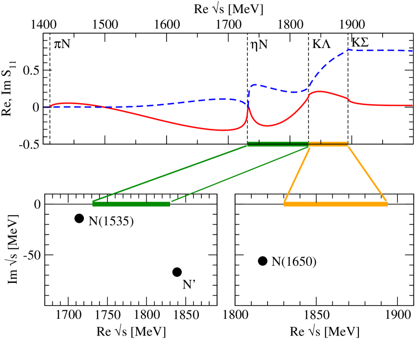
Figure 2: Upper panel: Real (solid line) and imaginary part (dashed line) of the $S_{11}$ amplitude, chirally extrapolated using masses and decay constants of the ETM collaboration. Lower panels: two of the Riemann sheets with poles. Labeling as in Fig. 1.

The $S_{11}$ amplitude, with the masses and decay constants of the ETM collaboration, is shown in the upper panel of Fig. 2. Comparing to Fig. 1, all thresholds have moved to higher energies. The cusp at the $\eta N$ threshold has become more pronounced, but no clear resonance shapes are visible. The structure of the amplitude becomes clearer by inspecting the complex energy plane on different Riemann sheets. This is visualized in the lower panels of Fig. 2. The Riemann sheets and labeling of the poles are the same as in Fig. 1. The pole positions are

$$W_{N(1535)}^{\rm Set~{}A} =(1714-i\,14)\text{ MeV (hidden)},$$

$$W_{N^{\prime}~{}~{}~{}~{}~{}~{}~{}}^{\rm Set~{}A} =(1839-i\,67)\text{ MeV (hidden)},$$

$$W_{N(1650)}^{\rm Set~{}A} =(1817-i\,56)\text{ MeV (hidden)}.$$ (19)

Compared to the physical point, the imaginary parts of the pole positions became much smaller due to the reduced phase space. Both the thresholds and the real parts of the pole positions have moved to higher energies. However, the thresholds have moved farther than the pole positions, such that the $N(1535)$ and $N(1650)$ poles are no longer situated below the part of the respective sheet, that is connected to the physical axis (thick horizontal lines). The poles are thus hidden and no clear resonance signals are visible in the physical amplitude. Instead, the amplitude is dominated by cusp effects.

Figure 3: Volume dependence of the energy levels predicted by our model for $I=1/2$ $\pi N$ scattering for periodic (upper) and antiperiodic (lower) boundary conditions. Masses and pion decay constant are taken from ETMC, see Refs. [60, 61].

Having analyzed the infinite-volume solution, we now turn to the finite-volume spectrum. By discretizing the model as outlined in Sec. 2.2 we obtain the prediction for the volume dependence of the energy levels shown in Fig. 3. In the upper panel, the spectrum for periodic boundary conditions is shown. The lowest level at the $\pi N$ threshold exhibits the characteristic $1/L^{3}$ dependence that can serve to calculate the (attractive) scattering length.

Similarly, the next level is situated close to the $\eta N$ threshold. This level is not induced by the presence of a resonance but a genuine effect of an $S$-wave threshold in a multi-channel problem. Such inelastic thresholds induce the same avoided level crossing as resonances, discussed in detail in Refs. [31, 32]. One striking example discussed there is the one of the $f_{0}(980)$ close to the $\bar{K}K$ thresholds: irrespectively of whether the resonance is present or not, there is avoided level crossing, and the levels are only slightly shifted if the resonance, albeit being so narrow, is present. Thus, the level below the $\eta N$ threshold shown in Fig. 3 cannot be attributed to the $N(1535)$ resonance. In any case, the $N(1535)$ is on a different sheet and, moreover, hidden as discussed following Fig. 2.

The following two levels, beyond the $\eta N$ threshold, are more difficult to interpret. They both show a plateau that, however, cannot be uniquely attributed neither to the $KY$ threshold nor to the hidden resonances. The rather involved interplay between hidden poles and threshold openings hinders the straightforward extraction of resonances.

The lower panel of Fig. 3 shows the level spectrum if antiperiodic boundary conditions are applied to the strange quark. As discussed in Sec. 2.2, this results in unchanged propagators for the $\pi N$ and $\eta N$ channels, while the $KY$ channels undergo modifications. In particular, the summation over lattice momenta is shifted from the origin, resulting in a finite relative momentum for the $KY$ pair at rest, of $\pm(\pi/L,\pi/L,\pi/L)$ [31]. Accordingly, the singularities at the $KY$ thresholds, induced by the denominator of $f$ in Eq. (10), are shifted and the avoided level crossing associated with $S$-wave thresholds disappears. Indeed, the third and fourth level, that showed avoided crossing with periodic boundary conditions, have a very different $L$-dependence with antiperiodic boundary conditions as Fig. 3 shows. In particular, the plateaus have disappeared.

Even for the second level, below the $\eta N$ threshold, we observe small changes of the $L$-dependence, even though the boundary conditions are only changed for the higher-lying $KY$ channels. This demonstrates that changes of the boundary conditions for the strange quark can indeed have an effect for the sub-threshold dynamics.

In summary, the resonance poles for the ETMC setup lie on hidden sheets. Plateaus of the $L$-dependence of the levels are rather tied to two-particle thresholds than to resonances, and neither with periodic nor antiperiodic boundary conditions a direct access to the $N(1535)$ or $N(1650)$ resonances is possible. In Sec. 3.3 we discuss strategies how to proceed in such a case.

3.2 Set B - QCDSF

Figure 4: Upper panel: Real (solid line) and imaginary part (dashed line) of the $S_{11}$ amplitude, chirally extrapolated using masses and decay constants of the QCDSF collaboration [62]. Lower panels: two of the Riemann sheets with poles. Labeling as in Fig. 1.

For the second set of parameters we choose a setup employed by the QCDSF collaboration [62]. Here, baryon and meson masses are determined from an alternative approach to tune the quark masses. Most importantly, while the lattice size and spacing are comparable to those of the ETMC, i.e. $L/a=32$ and $a=0.075$ fm, the strange quark mass differs significantly from the physical value. The latter results in a different ordering of the masses of the ground-state octet mesons and, consequently, in a different ordering of meson-baryon thresholds. For further details we refer the interested reader to Ref. [62]. Altogether, the lattice input for our calculation reads

$m_{N}^{\rm Set~{}B}=1020$,	$M_{\pi~{}}^{\rm Set~{}B}=286$,	$F_{\pi}^{\rm Set~{}B}=106.6$,
$m_{\Sigma}^{\rm Set~{}B}=1155$,	$M_{K~{}}^{\rm Set~{}B}=482$,	$F_{K}^{\rm Set~{}B}=115.3$,
$m_{\Lambda}^{\rm Set~{}B}=1111$,	$M_{\eta}^{\rm Set~{}B}=619$,	$F_{\eta}^{\rm Set~{}B}=127.6$,

where the meson decay constants have been calculated from next-to-leading order chiral perturbation theory. Two low-energy constants enter the calculation, for which the world lattice results were taken from [63], i.e. $L_{4}=0.04$ and $L_{5}=0.84$.

As discussed before, the NLO contributions become quite large already at energies slightly above the $\pi N$ threshold, adding up destructively with the contribution from the Weinberg-Tomozawa term. This reduces the scattering length compared to the one calculated with the physical parameters, like in the ETMC case. However, for the QCDSF values the $K\Sigma$ threshold lies closer to the $\pi N$ threshold than in the physical or in the ETMC set. Consequently, the $K\Sigma$ loops contribute stronger to the pion-nucleon scattering amplitudes, which yields an overall pion-nucleon scattering length of $a_{\pi N}^{1/2}=1.18$ GeV^-1. This is almost the size of the physical value and larger than in the ETMC set discussed before.

The scattering length depends on the input masses and decay constants, let alone the model dependence. However, for none of our parameter configurations we observe such a large $\pi N$ scattering length as reported by Lang and Verduci [18], their value being $5.3\pm 1.4$ GeV^-1.

The amplitude using the QCDSF parameter set is shown in the upper panel of Fig. 4. In contrast to the ETMC case, a clear resonance signal is visible below the $K\Lambda$ threshold, that is the first inelastic channel in this parameter setup. Indeed, we find a pole $N_{1}$ on the corresponding Riemann sheet, as indicated in the lower left panel. Unlike in the ETMC case, it is not hidden behind a threshold. Between the $K\Lambda$ and the $K\Sigma$ threshold, there is only the hidden pole $N_{2}$ (right panel). The $K\Sigma$ and $\eta N$ thresholds are almost degenerate and on sheets corresponding to these higher-lying thresholds we only find hidden poles. The precise pole positions are

$$W_{N_{1}}^{\rm Set~{}B}=(1562-i\,38)\text{ MeV},$$

$$W_{N_{2}}^{\rm Set~{}B}=(1479-i\,34)\text{ MeV (hidden)}.$$ (20)

Discretizing the present model as described in Sec. 2.2 we obtain the energy levels shown in Fig. 5.

Figure 5: Volume dependence of the energy levels predicted by our model for $I=1/2$ $\pi N$ scattering for periodic (upper) and antiperiodic (lower) boundary conditions. Masses and decay constants are taken from the calculation by the QCDSF collaboration, see Ref. [62].

For periodic boundary conditions (upper panel) we observe that most of energy levels are close to the two-particle thresholds for large $L$. At the position of the $N_{1}$ pole, there is a level. However, we have here a pole close to a threshold, with a second channel open. This is precisely the situation of the $f_{0}(980)$ discussed in depth in Ref. [32]. In the following section we discuss strategies to extract the amplitude in such cases.

Using antiperiodic boundary conditions for the strange quark, as shown in the lower panel of Fig. 5, the singularity at the $K\Lambda$ threshold is removed. In that case, we observe an almost $L$-independent level very close to the position of the $N_{1}$ pole. As the resonance is quite narrow, one might identify this level with the $N_{1}$ pole, although there are, of course, still finite-volume corrections.

While the extraction of the $N_{1}$ pole is quite promising for the parameters used by the QCDSF collaboration, one should still realize that this pole is on a different sheet than the one of the $N(1535)$ or the $N(1650)$. It is not evident what happens to this pole as the masses and decay constants approach the physical point and thus the various thresholds get ordered correctly.

3.3 Discussion and outlook

The negative parity $S_{11}$ partial wave in meson-baryon scattering is very complex due to many threshold openings and two resonances, one of which strongly coupling to the $\eta N$ channel. Those resonances are also believed to have a strong sub-threshold couplings to the $KY$ channels. Fitting the physical amplitude and thus fixing low-energy constants and scales, we use the quark mass dependence of the Weinberg-Tomozawa and the NLO contact terms to predict the amplitude for typical lattice setups. Depending on the masses and decay constants, resonance poles may become hidden behind thresholds as in case of the ETMC setup. In the QCDSF setup, there is one pole visible as a prominent resonance on the physical. However, in that setup the threshold ordering is reversed and it is not clear what happens to this pole as the quark masses are lowered.

For these amplitudes at unphysical quark masses, we have predicted the finite-volume level-spectrum. Resonances usually manifest themselves in avoided level crossing. However, in $S$-wave there is the additional complication that inelastic thresholds induce the same pattern. If resonances are close to thresholds, it is very difficult to disentangle the dynamics, as is observed for both setups studied. The effect of the $KY$ thresholds may be reduced by introducing twisted boundary conditions for the strange. Indeed, for the QCDSF setup we observe an almost $L$-independent level close to the resonance position. This shows that changing the boundary conditions promises indeed for a cleaner resonance extraction, although the technical realization on the lattice is intricate. In any case, modified boundary conditions for the strange quark shed light on the nature of the $J^{P}=1/2^{-}$ resonances and their supposed strong coupling to the hidden strangeness $KY$ channels.

In Ref. [32] it was discussed how to combine lattice data from different boundary conditions to extrapolate resonances in a two-channel problem to the infinite-volume limit. If one makes minimal assumptions on the smoothness of the potential, information from different energies may be combined to allow for a quantitative resonance extraction. A complimentary way to obtain more information from the lattice, without having to change the volume, is the use of moving frames. Unlike the $\pi\pi$ case, in meson-baryon scattering there are, however, many large higher partial waves of different parity, and the disentanglement of the $S$-wave contribution might become difficult.

In summary, we have shown that due to the many thresholds the $N(1535)$ and $N(1650)$ may become hidden in a unitary chiral extrapolation of the amplitude to unphysical quark masses. The extrapolation to the infinite volume poses additional problems due to a complicated threshold-resonance interplay requiring special techniques as modified boundary conditions to disentangle the resonance dynamics.

Acknowledgments We thank A. Rusetsky for useful discussions. This work is supported in part by the EU Integrated Infrastructure Initiative HadronPhysics3 and the DFG through funds provided to the Sino-German CRC 110 “Symmetries and the Emergence of Structure in QCD” and to the CRC 16 “Subnuclear Structure of Matter”.

References

- [1] N. Kaiser, P. B. Siegel and W. Weise, Phys. Lett. B 362 (1995) 23 [nucl-th/9507036].
- [2] T. Inoue, E. Oset and M. J. Vicente Vacas, Phys. Rev. C 65 (2002) 035204 [arXiv:hep-ph/0110333].
- [3] J. Nieves and E. Ruiz Arriola, Phys. Rev. D 64 (2001) 116008 [arXiv:hep-ph/0104307].
- [4] M. Döring, C. Hanhart, F. Huang, S. Krewald and U.-G. Meißner, Nucl. Phys. A 829 (2009) 170 [arXiv:0903.4337 [nucl-th]].
- [5] P. C. Bruns, M. Mai and U.-G. Meißner, Phys. Lett. B 697 (2011) 254 [arXiv:1012.2233 [nucl-th]].
- [6] H. Denizli et al. [CLAS Collaboration], Phys. Rev. C 76 (2007) 015204 [arXiv:0704.2546 [nucl-ex]].
- [7] E. F. McNicoll et al. [Crystal Ball at MAMI Collaboration], Phys. Rev. C 82 (2010) 035208 [Erratum-ibid. C 84 (2011) 029901] [arXiv:1007.0777 [nucl-ex]].
- [8] M. Mai, P. C. Bruns and U.-G. Meißner, Phys. Rev. D 86 (2012) 094033 [arXiv:1207.4923 [nucl-th]].
- [9] D. Ruic, M. Mai and U.-G. Meißner, Phys. Lett. B 704 (2011) 659 [arXiv:1108.4825 [nucl-th]].
- [10] D. Jido, M. Döring and E. Oset, Phys. Rev. C 77 (2008) 065207 [arXiv:0712.0038 [nucl-th]].
- [11] M. Döring and K. Nakayama, Eur. Phys. J. A 43 (2010) 83 [arXiv:0906.2949 [nucl-th]].
- [12] M. Döring and K. Nakayama, Phys. Lett. B 683 (2010) 145 [arXiv:0909.3538 [nucl-th]].
- [13] R. L. Workman, M. W. Paris, W. J. Briscoe, L. Tiator, S. Schumann, M. Ostrick and S. S. Kamalov, Eur. Phys. J. A 47 (2011) 143 [arXiv:1102.4897 [nucl-th]].
- [14] R. L. Workman, M. W. Paris, W. J. Briscoe and I. I. Strakovsky, Phys. Rev. C 86 (2012) 015202 [arXiv:1202.0845 [hep-ph]].
- [15] W. Chen, H. Gao, W. J. Briscoe, D. Dutta et al., Phys. Rev. C 86 (2012) 015206 [arXiv:1203.4412 [hep-ph]].
- [16] D. Drechsel, S. S. Kamalov and L. Tiator, Eur. Phys. J. A 34 (2007) 69 [arXiv:0710.0306 [nucl-th]].
- [17] B. Borasoy, P. C. Bruns, U.-G. Meißner and R. Nißler, Eur. Phys. J. A 34 (2007) 161 [arXiv:0709.3181 [nucl-th]].
- [18] C. B. Lang and V. Verduci, arXiv:1212.5055 [hep-lat].
- [19] R. W. Schiel, G. S. Bali, V. M. Braun, S. Collins, M. Gockeler, C. Hagen, R. Horsley and Y. Nakamura et al., PoS LATTICE 2011 (2011) 175 [arXiv:1112.0473 [hep-lat]].
- [20] J. Bulava et al., Phys. Rev. D 82 (2010) 014507 [arXiv:1004.5072 [hep-lat]].
- [21] S. Basak, R. G. Edwards, G. T. Fleming et al., Phys. Rev. D76 (2007) 074504 [arXiv:0709.0008 [hep-lat]].
- [22] G. P. Engel, C. B. Lang, M. Limmer, D. Mohler and A. Schäfer [BGR Collaboration], Phys. Rev. D 82 (2010) 034505 [arXiv:1005.1748 [hep-lat]].
- [23] N. Mathur, Y. Chen, S. J. Dong, T. Draper, I. Horvath, F. X. Lee, K. F. Liu and J. B. Zhang, Phys. Lett. B 605 (2005) 137 [hep-ph/0306199].
- [24] M. Lüscher, Commun. Math. Phys. 105 (1986) 153.
- [25] M. Lüscher, Nucl. Phys. B 354 (1991) 531.
- [26] U. J. Wiese, Nucl. Phys. Proc. Suppl. 9 (1989) 609.
- [27] V. Bernard, U.-G. Meißner and A. Rusetsky, Nucl. Phys. B 788 (2008) 1 [arXiv:hep-lat/0702012].
- [28] V. Bernard, M. Lage, U.-G. Meißner and A. Rusetsky, JHEP 0808 (2008) 024 [arXiv:0806.4495 [hep-lat]].
- [29] M. Lage, U.-G. Meißner and A. Rusetsky, Phys. Lett. B 681 (2009) 439 [arXiv:0905.0069 [hep-lat]].
- [30] C. Liu, X. Feng and S. He, Int. J. Mod. Phys. A 21 (2006) 847 [hep-lat/0508022].
- [31] V. Bernard, M. Lage, U.-G. Meißner and A. Rusetsky, JHEP 1101 (2011) 019 [arXiv:1010.6018 [hep-lat]].
- [32] M. Döring, U.-G. Meißner, E. Oset and A. Rusetsky, Eur. Phys. J. A 47 (2011) 139 [arXiv:1107.3988 [hep-lat]].
- [33] N. Li and C. Liu, Phys. Rev. D 87 (2013) 014502 [arXiv:1209.2201 [hep-lat]].
- [34] J. M. M. Hall, A. C. -P. Hsu, D. B. Leinweber, A. W. Thomas and R. D. Young, PoS LATTICE 2012 (2012) 145 [arXiv:1207.3562 [hep-lat]].
- [35] R. A. Arndt, W. J. Briscoe, I. I. Strakovsky, R. L. Workman and M. M. Pavan, Phys. Rev. C 69 (2004) 035213 [nucl-th/0311089].
- [36] J. Beringer et al. [Particle Data Group Collaboration], Phys. Rev. D 86 (2012) 010001.
- [37] S. R. Beane, P. F. Bedaque, A. Parreno et al., Nucl. Phys. A747 (2005) 55 [arXiv:nucl-th/0311027].
- [38] M. Döring, J. Haidenbauer, U.-G. Meißner and A. Rusetsky, Eur. Phys. J. A 47 (2011) 163 [arXiv:1108.0676 [hep-lat]].
- [39] A. Martinez Torres, M. Bayar, D. Jido and E. Oset, Phys. Rev. C 86 (2012) 055201 [arXiv:1202.4297 [hep-lat]].
- [40] F. Okiharu et al., arXiv:hep-ph/0507187; H. Suganuma, K. Tsumura, N. Ishii and F. Okiharu, PoS LAT2005 (2006) 070 [arXiv:hep-lat/0509121]; H. Suganuma, K. Tsumura, N. Ishii and F. Okiharu, Prog. Theor. Phys. Suppl. 168 (2007) 168 [arXiv:0707.3309 [hep-lat]].
- [41] D. Morgan and M. R. Pennington, Phys. Rev. D 48, 1185 (1993).
-
[42]
V. Baru, J. Haidenbauer, C. Hanhart, A. E. Kudryavtsev and
U.-G. Meißner, Eur. Phys. J. A 23 (2005) 523 [arXiv:nucl-th/0410099]. - [43] D. Rönchen, et al., arXiv:1211.6998 [nucl-th].
- [44] M. Döring, C. Hanhart, F. Huang, S. Krewald, U.-G. Meißner and D. Rönchen, Nucl. Phys. A 851 (2011) 58 [arXiv:1009.3781 [nucl-th]].
- [45] S. Kreuzer and H.-W. Hammer, Phys. Lett. B 694 (2011) 424 [arXiv:1008.4499 [hep-lat]].
- [46] K. Polejaeva and A. Rusetsky, Eur. Phys. J. A 48 (2012) 67 [arXiv:1203.1241 [hep-lat]].
- [47] L. Roca and E. Oset, Phys. Rev. D 85 (2012) 054507 [arXiv:1201.0438 [hep-lat]].
- [48] P. Guo, J. Dudek, R. Edwards and A. P. Szczepaniak, arXiv:1211.0929 [hep-lat].
- [49] R. A. Briceño and Z. Davoudi, arXiv:1212.3398 [hep-lat].
- [50] K. Rummukainen and S. A. Gottlieb, Nucl. Phys. B 450 (1995) 397. [hep-lat/9503028].
- [51] S. Bour, S. König, D. Lee, H.-W. Hammer and U.-G. Meißner, Phys. Rev. D 84 (2011) 091503. [arXiv:1107.1272 [nucl-th]].
- [52] Z. Davoudi and M. J. Savage, Phys. Rev. D 84 (2011) 114502 [arXiv:1108.5371 [hep-lat]].
- [53] Z. Fu, Phys. Rev. D 85 (2012) 014506. [arXiv:1110.0319 [hep-lat]].
- [54] C. S. Pelissier, A. Alexandru and F. X. Lee, PoS LATTICE 2011 (2011) 134 [arXiv:1111.2314 [hep-lat]].
- [55] L. Leskovec and S. Prelovsek, Phys. Rev. D 85 (2012) 114507 [arXiv:1202.2145 [hep-lat]].
- [56] J. J. Dudek, R. G. Edwards and C. E. Thomas, Phys. Rev. D 86 (2012) 034031 [arXiv:1203.6041 [hep-ph]].
- [57] R. A. Briceño and Z. Davoudi, arXiv:1204.1110 [hep-lat].
- [58] M. Döring, U.-G. Meißner, E. Oset and A. Rusetsky, Eur. Phys. J. A 48 (2012) 114 [arXiv:1205.4838 [hep-lat]].
- [59] M. Göckeler, R. Horsley, M. Lage, U.-G. Meißner, P. E. L. Rakow, A. Rusetsky, G. Schierholz and J. M. Zanotti, Phys. Rev. D 86 (2012) 094513 [arXiv:1206.4141 [hep-lat]].
- [60] K. Ottnad et al. [ETM Collaboration], JHEP 1211 (2012) 048 [arXiv:1206.6719 [hep-lat]].
- [61] C. Alexandrou et al. [ETM Collaboration], Phys. Rev. D 80 (2009) 114503 [arXiv:0910.2419 [hep-lat]].
- [62] W. Bietenholz, et al., Phys. Rev. D 84 (2011) 054509 [arXiv:1102.5300 [hep-lat]].
- [63] G. Colangelo, et al., Eur. Phys. J. C 71 (2011) 1695 [arXiv:1011.4408 [hep-lat]].