Dissipative soliton excitability induced by spatial inhomogeneities and drift

Abstract

We show that excitability is generic in systems displaying dissipative solitons when spatial inhomogeneities and drift are present. Thus, dissipative solitons in systems which do not have oscillatory states, such as the prototypical Swift-Hohenberg equation, display oscillations and Type I and II excitability when adding inhomogeneities and drift to the system. This rich dynamical behavior arises from the interplay between the pinning to the inhomogeneity and the pulling of the drift. The scenario presented here provides a general theoretical understanding of oscillatory regimes of dissipative solitons reported in semiconductor microresonators. Our results open also the possibility to observe this phenomenon in a wide variety of physical systems.

Spatially extended systems display a large variety of emergent behaviors Cross and Hohenberg (1993), including coherent structures. Particularly interesting is the case of dissipative solitons (DS) Akhmediev and Ankiewicz (2005); *Akhmediev2, exponentially localized structures in dissipative systems driven out of equilibrium, as they can behave like discrete objects in continuous systems. DS can display a variety of dynamical regimes such as periodic oscillations Umbanhowar et al. (1996); Firth et al. (1996); *Firth2; Vanag and Epstein (2007), chaos Michaelis et al. (2003); Gelens et al. (2012), or excitability Gomila et al. (2005); *Gomila05b. DS emerge from a balance between nonlinearity and spatial coupling, and driving and dissipation. They are unique once the system parameters are fixed, and they are different from the well known conservative solitons that appear as one-parameter families.

In optical cavities, DS (also known as cavity solitons) have been proposed as bits for all-optical memories Firth and Weiss (2002); Barland et al. (2002); Pedaci et al. (2008); Leo et al. (2010); Odent et al. (2011), due to their spatial localization and bistable coexistence with the fundamental solution. In Ref. Gomila et al. (2005); *Gomila05b it was reported that DS may exhibit excitable behavior. A system is said to be excitable if perturbations below a certain threshold decay exponentially, while perturbations above this threshold induce a large response before going back to the resting state. Excitability is found for parameters close to those where a limit cycle disappears Izhikevich (2007). Excitability mediated by DS is different from the well known dynamics of excitable media, whose behavior stems from the (local) excitability present in the system without spatial degrees of freedom. Excitability of DS is an emergent behavior, arising through the spatial interaction and not present locally. Moreover, the interaction between different excitable DS can be used to build all-optical logical gates Jacobo et al. (2012).

In real systems, however, typically solitons are static, so oscillatory or excitable DS are far from being generic. In this work we present a mechanism that generically induces dynamical regimes, such as oscillations and excitable behavior, in which the structure of the DS is preserved. The mechanism relies on the interplay between spatial inhomogeneities and drift, and therefore can be implemented under very general conditions. Inhomogeneities, or defects, are unavoidable in any experimental setup, and drift is also often present in many optical, fluid and chemical systems, due to misalignments of the mirrors Santagiustina et al. (1997); Louvergneaux et al. (2004), nonlinear crystal birefringence Ward et al. (1998); *walk-off2, or parameter gradients Schapers et al. (2003), in the first case, and due to the flow of a fluid in the others Babcock et al. (1991); von Haeften and Izús (2003). Roughly speaking, the presence of inhomogeneities and drift introduce two competing effects. On the one hand, an inhomogeneity pins a DS at a fixed position and, on the other, the drift tries to pull it out. If the drift overcomes the pinning, DS solitons are released from the inhomogeneity Schapers et al. (2003); Caboche et al. (2009a); *Caboche2. Thus, depending on the height of the spatial inhomogeneity and the strength of the drift, we observe three main dynamical regimes: i) stationary (pinned) solutions, ii) oscillatory regimes, where DS source continuously from the inhomogeneity, and iii) excitability, where a perturbation may trigger a single DS that is driven away from the inhomogeneity. This scenario does not depend on the details of the system nor on the spatial dimensionality. Besides, it provides a solid theoretical framework to explain the dynamics of DS in systems with drift, as observed for instance in semiconductor microresonators Pedaci et al. (2008); Caboche et al. (2009a); *Caboche2.

To analyze this scenario we start with the prototypical Swift-Hohenberg equation (SHE), a generic amplitude equation describing pattern formation in a large variety of systems Cross and Hohenberg (1993); Tlidi et al. (1994); Woods and Champneys (1999); Burke and Knobloch (2007). The SHE is variational, thus it can not have oscillatory regimes. Adding drift and a spatial inhomogeneity we have:

$$\frac{\partial u}{\partial t}=-\left(\frac{\partial^{2}}{\partial x^{2}}+k_{0}^{2}\right)^{2}u+c\frac{\partial u}{\partial x}+r(x)u+au^{2}-gu^{3}+b(x).$$ (1)

Here $u(x,t)$ is a real field, $a$ and $g$ real parameters, and $c$ is the velocity of the drift. The SHE displays DS for $a>\sqrt{27/38}g$ Woods and Champneys (1999); Burke and Knobloch (2007), so we take $a=1.2$ and $g=1$. We fix $k_{0}^{2}=0.5$. We use a supergaussian gain profile $r(x)=r_{0}-1+\exp\{-\left[(x-x_{0})/\epsilon\right]^{18}\}$ to model a finite system of width $2\epsilon$ so that DS disappear at the boundaries. We fix $r_{0}=-0.2$, roughly in the middle of the subcritical region where DS exist, and, except where otherwise indicated, $\epsilon=94.0842$. Small changes of the parameter values do not substantially modify the results. A single spatial inhomogeneity located at the center is introduced adding a Gaussian profile $b(x)=h\exp\{-\left[(x-x_{0})/\sigma\right]^{2}\}$ with height $h$ and half-width $\sigma$ Jacobo et al. (2008). This is motivated by the addressing beams used in optical systems to control DS Barland et al. (2002); Brambilla et al. (1996); *defects2. We take $\sigma=2.045$, roughly half the width of a DS. Similar results are found for other values of $\sigma$ provided the width is small enough to avoid trapping two DS. We have also checked that similar results are found for a defect in the gain profile $r$. We take $h$ and $c$ as control parameters .

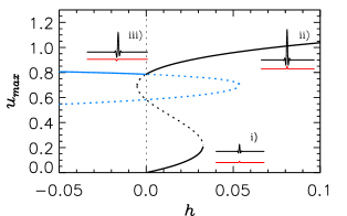
Figure 1: (Color online) Bifurcation diagram showing the maximum of the steady state, $u_{max}$, as a function of $h$ for $c=0$. In black solutions pinned at their center and in gray (blue) DS pinned at the first tail minima. Solid (dashed) lines indicate stable (unstable) solutions. The insets show the profiles of the solution and the spatial inhomogeneity.

For $c=0$ we observe three different steady state solutions which are the main attractors of the dynamics (Fig. 1): i) the fundamental solution, a low bump corresponding to the deformation of the homogeneous solution, ii) a high amplitude DS pinned at its center, and iii) a DS pinned at the first oscillation of its tail. Decreasing $h$, at $h=0$, a transcritical bifurcation occurs in which branch ii) becomes unstable while iii) is stabilized. Physically, at $h=0$ the defect goes from being a bump to a hole. DS tend to sit at the inhomogeneity maximum, thus a DS centered at the hole becomes unstable and shifts its position until the hole coincides with the first minimum of its tail . At $h=0$ there is also a crossing of unstable middle-branch DS. In what follows we focus on $h>0$.

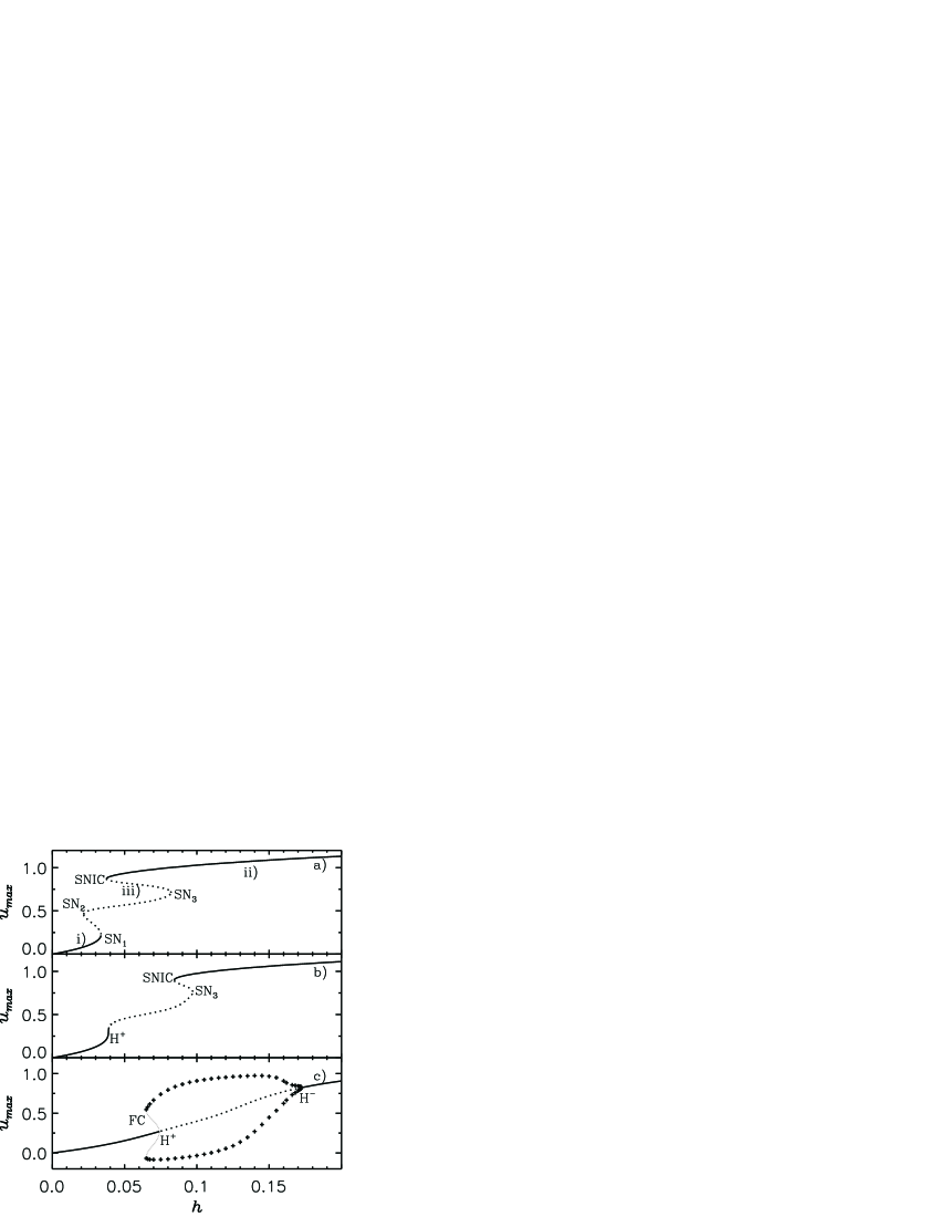
Figure 2: The same as in Fig. 1 for a) $c=0.05$, b) $c=0.12$ and c) $c=0.4$ (see main text). In c) the crosses indicate the maximum and minimum value of the oscillatory DS at a given spatial location. The grey dotted line is a sketch of the unstable cycle for illustrative purposes.

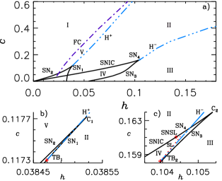
Figure 3: a) (Color online) Two-parameter ($c$ vs $h$) phase diagram of the system (see text). Panels b) and c) show a zoom close to the cusps and Takens-Bogdanov points.

This scenario changes when drift is introduced, $c\neq 0$: parity symmetry, $x\leftrightarrow-x$, is broken making the transcritical bifurcations imperfect. This implies a rearrangement of branches, that for low values of $c$ leads to the snake-like branch shown in Fig. 2a). Saddle-node bifurcations SN₁ and SN₃ where already present for $c=0$. A Saddle-Node on the Invariant Circle (SNIC) reconnects branches ii) and iii), while the saddle-node SN₂ arises from the middle branches transcritical bifurcation. Increasing $c$ the branch stretches (cf. Fig. 2b) and SN₁ coalesces with SN₂ at the cusp bifurcation C₁ as shown in Fig. 3 which displays the general scenario in parameter space. Close to C₁ there is a Takens-Bogdanov point TB₁ that unfolds a Hopf bifurcation line H⁺ Gelens et al. (2008) (Fig. 3b). As $c$ keeps increasing, the SNIC line encounters a Saddle-Node Separatrix Loop (SNSL) codimension 2 bifurcation from which a saddle-node SN₄ and a saddle-loop SL bifurcation lines unfold (Fig. 3c). SN₄ soon coalesces with SN₃ at the cusp C₂ while SL ends at a Takens-Bogdanov point, TB₂, which also unfolds a Hopf line H^- tangent to the SL line. Finally for larger values of $c$ there is a single monotonous branch of steady state solutions (Fig. 2c). The Hopf line H⁺ is subcritical and is accompanied by a fold of cycles (FC) from which a stable cycle emerges. For $h$ large enough the defect is above the threshold to switch on a DS. Thus this limit cycle corresponds to the periodic creation of DS at the inhomogeneity that are then drifted away (Fig. 4c), generating a train of solitons that, in our case, disappear at the boundary of the system (Fig. 4a). Such regime was observed experimentally in semiconductor microresonators Caboche et al. (2009a); *Caboche2, where it was called a “soliton tap”. This cycle is stable all the way to the supercritical Hopf H^-, where $h$ becomes large enough to prevent the DS being advected by the drift, and the cycle ends.

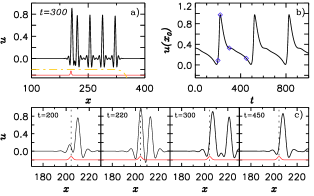
Figure 4: a) (Color online) Snapshot of a train of solitons in region II of Fig. 3 for $c=0.11$ and $h=0.076$. The solid grey (red) and the dot-dashed lines show $b(x)$ and $r(x)$ respectively. Here $\epsilon=163.625$. b) Time evolution of the field $u$ at $x_{0}$. c) Field profile at the times shown with symbols in b) showing how a new DS develop and detach.

In parameter space (Fig. 3) the fundamental solution is stable in regions I and V, pinned DS are stable in III and IV and stable trains of DS exist in II and V. The scenario shown in Figs. 3b and 3c, much richer than in Gomila et al. (2005); *Gomila05b, is characteristic of systems displaying relaxation oscillations described, for instance, by the Van der Pol equation (see Fig. 2.1.2 in Guckenheimer and Holmes (1983)). These systems are characterized by two different time scales, a slow and a fast one. Here the fast time scale corresponds to the switching time of a DS on the inhomogeneity, while the slow one is the time the drift takes to detach a DS once it is formed Caboche et al. (2009a); *Caboche2. The switch-on time is basically independent on the drift, while the detach time has a strong dependence on it. These two time scales can be clearly identified in a time trace of the field at $x_{0}$ (Fig. 4b). Excitability can be found in regions I, III and IV when applying a perturbation for a short time that changes either $c$ or $h$. If the system is brought monetarily into the oscillatory region II then an excitable excursion consisting on the exploration of a loop of the cycle before returning to the original steady state is triggered. An alternative way to trigger an excitable excursion is perturbing the state of the system rather than a parameter Izhikevich (2007). Transient parameter changes are usually easier to implement experimentally, thus in what follows we consider this kind of perturbations.

In region I a superthreshold perturbation of the fundamental solution grows to generate a DS, that is then advected away, setting the defect back to the resting state (Fig. 5). As the transition from the stationary state to the oscillatory one is mediated by a subcritical Hopf bifurcation, the excitability is of Type II Izhikevich (2007). A clear signature of this type of excitability is that the period of the oscillations remains practically constant as one approaches the threshold from the oscillatory side, namely as one approaches FC coming from region II, as shown in Fig. 6a. As typical for Type II excitability the threshold is rather a quasi-threshold. If one applies a perturbation that crosses FC but not H⁺, the system will be stacked in region V (bistable). The closer the parameters are to FC, and the closer is FC to H⁺, the smaller is the perturbation required to trigger an excitable excursion .

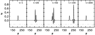
Figure 5: Excitable excursion of the fundamental solution in region I, close to FC ($c=0.6$, $h=0.085$), triggered varying $h$ an amount $\Delta h=0.0325$ during $\Delta t=20$ time units. The dot-dashed line shows the gain profile $r(x)$.

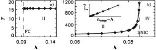
Figure 6: Oscillation period $T$ in region II as a function of $h$ close to a) the FC ($c=0.6$) and b) the SNIC ($c=0.12$). The inset in b) shows the scaling of the divergence of the period.

Different dynamics is found in region III, where $h$ is large enough that, beyond switching on a DS if there is none, it also pins it once it is formed. In this case DS undergo a supercritical Hopf bifurcation when crossing H^-. Close to threshold, DS exhibit small oscillations, but decreasing $h$ or increasing $c$ just a little further DS start to source from the inhomogeneity, forming a sort of canard in phase space Bold et al. (2003), leading to the train of DS found in region II. This is again a mechanism leading to Type II excitability as shown in Fig. 7. At difference with the previous case, here the resting state is a high amplitude DS (see first panel), and the excitable excursion consists of the DS leaving the inhomogeneity and a new one being formed.

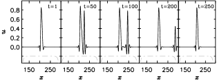
Figure 7: The same as in Fig.5 but close to H^-, in region III. Here $c=0.4$, $h=0.18$, and $\Delta h=-0.045$.

There is a third mechanism, associated to the SNIC line separating regions II and IV. A detailed analysis of DS excitability mediated by a SNIC can be found in Ref. Jacobo et al. (2008). For parameters in region IV a supra-treshold perturbation that brings the system into region II triggers the unpinning of a DS leading to an excitable excursion. The initial and the final state is a pinned DS and the observed behavior is very similar to the one shown in Fig. 7. In this case excitability is of Type I, whose signature is a divergence of the period. As shown in Fig. 6b) the period diverges with a power law of exponent $-1/2$ approaching the SNIC line from region II. A divergence in the period has been reported in semiconductor microresonators Caboche et al. (2009a); *Caboche2, induced also through spatial inhomogeneities and drift. Additionally, the SL line in Fig. 3c) leads to another Type I excitable region (discussed at length in Gomila et al. (2005); *Gomila05b), but at difference with the SNIC bifurcation line, that extends for a wide parameter range, the SL occurs in a very narrow region (Fig. 3c), and therefore it may be more difficult to find experimentally.

In summary, we have shown that the competition between the pinning of DS to a spatial inhomogeneity and the pulling generated by a drift leads to a complex behavior leading to oscillations and to Type I and II excitability through several mechanisms. To clearly illustrate this we make use of the SHE, for which there is a Lyapunov potential Cross and Hohenberg (1993), thus the system always evolves to steady states that minimize the potential. When drift and boundary conditions are added, the SHE no longer has a Lyapunov potential Cossu and Chomaz (1997), thus complex dynamical behavior can arise. In order to confirm the generality of our results, we have checked that the scenario is qualitatively the same in a completely different model displaying DS Gomila et al. (2007b), namely the Lugiato-Lefever equation Lugiato and Lefever (1987), which has been recently used to describe DS observed experimentally Leo et al. (2010); Odent et al. (2011). Our results do not depend on the microscopic details of the system, or the number of spatial dimensions, or the nature of the spatial inhomogeneity, but on general emergent properties of DS, providing a theoretical framework to explain the dynamics of DS in presence of spatial inhomogeneities and drift in a very broad class of extended systems. The theory presented here gives an explanation to experimental observations Caboche et al. (2009a); *Caboche2 and opens up the possibility to observe this phenomenon in a variety of other experimental setups.

Financial support from the MINECO (Spain) and FEDER under grants FIS2007-60327 (FISICOS) and TEC2009-14101 (DeCoDicA), FIS2012-30634 (INTENSE@COSYP), and TEC2012-36335 (TRIPHOP), from CSIC (Spain) under grants 200450E494 (Grid-CSIC) and PIE-201050I016, and from Comunitat Autònoma de les Illes Balears is acknowledged.

References

- Cross and Hohenberg (1993) M. Cross and P. Hohenberg, Rev. Mod. Phys. 65, 851 (1993).
- Akhmediev and Ankiewicz (2005) N. Akhmediev and A. Ankiewicz, eds., Dissipative Solitons, Lecture Notes in Physics, Vol. 661 (Springer, New York, 2005).
- Akhmediev and Ankiewicz (2008) N. Akhmediev and A. Ankiewicz, eds., Dissipative Solitons: From Optics to Biology and Medicine, Lecture Notes in Physics, Vol. 751 (Springer, New York, 2008).
- Umbanhowar et al. (1996) P. B. Umbanhowar, F. Melo, and H. L. Swinney, Nature 382, 793 (1996).
- Firth et al. (1996) W. J. Firth, A. Lord, and A. J. Scroggie, Phys. Scr. T67, 12 (1996).
- Firth et al. (2002) W. J. Firth, G. K. Harkness, A. Lord, J. McSloy, D. Gomila, and P. Colet, J. Opt. Soc. Am. B 19, 747 (2002).
- Vanag and Epstein (2007) V. K. Vanag and I. R. Epstein, Chaos 17, 037110 (2007).
- Michaelis et al. (2003) D. Michaelis, U. Peschel, C. Etrich, and F. Lederer, IEEE J. Quantum Electron. 39, 255 (2003).
- Gelens et al. (2012) L. Gelens, F. Leo, P. Emplit, M. Haelterman, and S. Coen, IEEE Photon. Conf. (IPC) , 364 (2012).
- Gomila et al. (2005) D. Gomila, M. A. Matías, and P. Colet, Phys. Rev. Lett. 94, 063905 (2005).
- Gomila et al. (2007a) D. Gomila, A. Jacobo, M. A. Matías, and P. Colet, Phys. Rev. E 75, 026217 (2007a).
- Firth and Weiss (2002) W. J. Firth and C. O. Weiss, Opt. Photonics News 13, 55 (2002).
- Barland et al. (2002) S. Barland, J. R. Tredicce, M. Brambilla, L. A. Lugiato, S. Balle, M. Giudici, T. Maggipinto, L. Spinelli, G. Tissoni, T. Knoedl, and M. Miller, Nature (London) 419, 699 (2002).
- Pedaci et al. (2008) F. Pedaci, S. Barland, E. Caboche, P. Genevet, M. Giudici, J. R. Tredicce, T. Ackemann, A. Scroggie, W. Firth, G. L. Oppo, G. Tissoni, and R. Jaeger, Appl. Phys. Lett. 92, 011101 (2008).
- Leo et al. (2010) F. Leo, S. Coen, P. Kockaert, S. P. Gorza, P. Emplit, and M. Haelterman, Nature Photonics 4, 471 (2010).
- Odent et al. (2011) V. Odent, M. Taki, and E. Louvergneaux, New J. Physics 13, 113026 (2011).
- Izhikevich (2007) E. M. Izhikevich, Dynamical Systems in Neuroscience: The Geometry of Excitability and Bursting (MIT Press, Cambridge (MA), 2007).
- Jacobo et al. (2012) A. Jacobo, D. Gomila, M. A. Matías, and P. Colet, New J. Physics 14, 013040 (2012).
- Santagiustina et al. (1997) M. Santagiustina, P. Colet, M. S. Miguel, and D. Walgraef, Phys. Rev. Lett. 79, 3633 (1997).
- Louvergneaux et al. (2004) E. Louvergneaux, C. Szwaj, G. Agez, P. Glorieux, and M. Taki, Phys. Rev. Lett. 92, 043901 (2004).
- Ward et al. (1998) H. Ward, M. N. Ouarzazi, M. Taki, and P. Glorieux, Eur. Phys. J. D 3, 275 (1998).
- Santagiustina et al. (1998) M. Santagiustina, P. Colet, M. S. Miguel, and D. Walgraef, Opt. Lett. 23, 1167 (1998).
- Schapers et al. (2003) B. Schapers, T. Ackemann, and W. Lange, IEEE J. Quantum Electron. 39, 227 (2003).
- Babcock et al. (1991) K. L. Babcock, G. Ahlers, and D. S. Cannell, Phys. Rev. Lett. 67, 3388 (1991).
- von Haeften and Izús (2003) B. von Haeften and G. Izús, Phys. Rev. E 67, 056207 (2003).
- Caboche et al. (2009a) E. Caboche, F. Pedaci, P. Genevet, S. Barland, M. Giudici, J. Tredicce, G. Tissoni, and L. A. Lugiato, Phys. Rev. Lett. 102, 163901 (2009a).
- Caboche et al. (2009b) E. Caboche, S. Barland, M. Giudici, J. Tredicce, G. Tissoni, and L. A. Lugiato, Phys. Rev. A 80, 053814 (2009b).
- Tlidi et al. (1994) M. Tlidi, P. Mandel, and R. Lefever, Phys. Rev. Lett. 73, 640 (1994).
- Woods and Champneys (1999) P. Woods and A. R. Champneys, Physica D 129, 147 (1999).
- Burke and Knobloch (2007) J. Burke and E. Knobloch, Chaos 17, 037102 (2007).
- Jacobo et al. (2008) A. Jacobo, D. Gomila, M. A. Matías, and P. Colet, Phys. Rev. A 78, 053821 (2008).
- Brambilla et al. (1996) M. Brambilla, L. Lugiato, and M. Stefani, Europhys. Lett. 34, 109 (1996).
- Spinelli et al. (1998) L. Spinelli, G. Tissoni, M. Brambilla, F. Prati, and L. A. Lugiato, Phys. Rev. A 58, 2542 (1998).
- Note (1) We consider periodic boundary conditions with a system size larger than the gain region. Numerical simulations are performed using a pseudospectral method. Starting from the steady state of a numerical simulation, bifurcation diagrams are found using a Newton method and continuation techniques (See Ref. Gomila et al. (2005); *Gomila05b). Stability is determined from the Jacobian eigenvalues.
- Note (2) Branch iii) corresponds to pinned DS whose maximum is at the right of the defect. There is also a degenerated branch with the maximum at the left. When the drift is turned-on the degeneracy is broken. We focus in the DS whose maximum is located downstream, since this branch reconnects to branch ii) when drift is applied.
- Gelens et al. (2008) L. Gelens, D. G. G. V. der Sande, J. Danckaert, P. Colet, and M. A. Matías, Phys. Rev. A 77, 033841 (2008).
- Guckenheimer and Holmes (1983) J. Guckenheimer and P. Holmes, Nonlinear Oscillations, Dynamical Systems, and Bifurcations of Vector Fields (Springer, New York, 1983).
- Note (3) The system is excitable even for , although in this case very large perturbations are required to trigger an excitable excursion.
- Bold et al. (2003) K. Bold, C. Edwards, J. Guckenheimer, S. Guharay, K. Hoffman, J. Hubbard, R. Oliva, and W. Weckesser, SIAM J. Appl. Dyn. Syst. 2, 570 (2003).
- Cossu and Chomaz (1997) C. Cossu and J. Chomaz, Phys. Rev. Lett. 78, 4387 (1997).
- Gomila et al. (2007b) D. Gomila, A. J. Scroggie, and W. J. Firth, Physica D 227, 70 (2007b).
- Lugiato and Lefever (1987) L. A. Lugiato and R. Lefever, Phys. Rev. Lett. 58, 2209 (1987).