Canonical Thermal Pure Quantum State
Abstract
A thermal equilibrium state of a quantum many-body system can be represented by a typical pure state, which we call a thermal pure quantum (TPQ) state. We construct the canonical TPQ state, which corresponds to the canonical ensemble of the conventional statistical mechanics. It is related to the microcanonical TPQ state, which corresponds to the microcanonical ensemble, by simple analytic transformations. Both TPQ states give identical thermodynamic results, if both ensembles do, in the thermodynamic limit. The TPQ states corresponding to other ensembles can also be constructed. We have thus established the TPQ formulation of statistical mechanics, according to which all quantities of statistical-mechanical interest are obtained from a single realization of either TPQ state. We also show that it has great advantages in practical applications. As an illustration, we study the spin-1/2 kagome Heisenberg antiferromagnet (KHA).
pacs:
05.30.-d, 75.10.Jm, 05.70.Ce, 02.70.-cStatistical mechanics is conventionally described by the ensemble formulation, in which an equilibrium state is represented by a mixed quantum state. Although its basic principles are introduced in the microcanonical ensemble, one can derive other ensembles, such as the canonical ensemble. This makes statistical mechanics powerful and practical because for most applications the (grand) canonical ensemble is more convenient than the microcanonical one.
On the other hand, recent studies have shown that almost all pure quantum states in a specified energy shell represent an equilibrium state Popescu ; Lebowitz ; SugitaJ ; SugitaE ; Reimann . Generalizing this fact, we have defined a TPQ state as a pure quantum state which represents an equilibrium state, and proposed a new formulation of statistical mechanics based on the TPQ state SS2012 . Since the TPQ state proposed there corresponds to the microcanonical ensemble, we here call it the microcanonical TPQ state. Then, natural questions arise: Are there TPQ states which correspond to other ensembles? How are they related to each other?
In this Letter, we construct a new type of TPQ state, the canonical TPQ state, which corresponds to the canonical ensemble. We show that it is related to the microcanonical TPQ state by simple analytic transformations. The TPQ states corresponding to other ensembles, such as the grand canonical ensemble, can also be constructed in a similar manner. These results establish the new formulation of statistical mechanics, which enables one to obtain all quantities of statistical-mechanical interest from a single realization of a TPQ state. This formulation is not only interesting as fundamental physics but also advantageous in practical applications because one needs only to construct a single pure state by just multiplying the Hamiltonian matrix to a random vector. The canonical TPQ state is particularly advantageous at low but finite temperature, whereas the microcanonical one is suitable for first-order phase transitions. As an illustration, we study the KHA using the canonical TPQ state.
Setup and definition – We consider a quantum system composed of sites or particles. By using an effective model in the energy scale of interest discrete , we describe the system with a Hilbert space of dimension , where Theta . [ for spin- systems.] To take the thermodynamic limit, we use quantities per site, and , where denotes the Hamiltonian and the energy. We do not write explicitly variables other than and , such as a magnetic field. We assume that the ensemble formulation gives correct results, which are consistent with thermodynamics in the thermodynamic limit. [Here, the term ‘thermodynamics’ is used in the sense of textbooks Callen ; TD .] This implies, e.g., that the entropy density is a concave function and that the equivalence of ensembles holds. A huge class of systems, excluding some models with long-range interactions TD ; Thirring , satisfy this condition.
Statistical mechanics treats macroscopic variables, which include ‘mechanical’ and ‘genuine thermodynamic’ ones. Mechanical variables, such as energy and spin-spin correlation functions, are the observables that are low-degree polynomials (i.e., their degree , where ) of local operators. In order to exclude foolish operators (such as ), we assume that every mechanical variable is normalized such that , where is a constant independent of and . By contrast, genuine thermodynamic variables, such as temperature and thermodynamic functions, cannot be represented as such operators. All genuine thermodynamic variables can be derived from the entropy function.
We have defined a TPQ state for the case where it has a random variable(s), as follows SS2012 . A state () is called a TPQ state if uniformly for every mechanical variable as . Here, , is the ensemble average, and ‘’ denotes convergence in probability. That is, for an arbitrary positive number there exists a function that vanishes in the thermodynamic limit and satisfies for every mechanical variable . [ denotes the probability of event .] This means that for sufficiently large just a single realization of gives the equilibrium values of all mechanical variables. Note that is never obtained by ‘purification’ of the density operator of the ensemble formulation, because is not a vector in an enlarged Hilbert space but a vector in .
Canonical TPQ state – We have previously constructed the microcanonical TPQ state, which is specified by (i.e., independent variables are ) SS2012 . We now construct the canonical TPQ state, which is specified by , for finite inverse temperature .
We take an arbitrary orthonormal basis of , , which can be a trivial one such as a set of product states. We also take random complex numbers , which are drawn uniformly from the unit sphere . Then, is a random vector in . Note that this construction of is independent of the choice of . We will show that
| (1) |
is the (unnormalized) canonical TPQ state specified by . We start with the rather obvious equality;
| (2) |
where denotes the random average, , and . To investigate how fast converges to this value, we evaluate with the help of formulas in Ref. Ullah . Dropping smaller-order terms, we find SpMt
| (3) |
where , and is the free energy density. We here use instead of to indicate that approaches the -independent one, , in the thermodynamic limit. Since , and at finite (because the entropy density ), we find , which becomes exponentially small with increasing .
On the other hand, a generalized Markov’s inequality yields, for arbitrary ,
| (4) |
The right-hand side , which vanishes exponentially fast with increasing , for every mechanical variable . Therefore, uniformly, which shows that is the canonical TPQ state.
Genuine thermodynamic variables – We now show that also gives genuine thermodynamic variables correctly. In the ensemble formulation, the partition function gives . Similarly, in our formulation the squared norm of gives as SpMt
| (5) | |||
| (6) |
Therefore, , and a single realization of the canonical TPQ state gives , with exponentially small probability of error, by
| (7) |
All genuine thermodynamic variables can be calculated from alsoMech . Furthermore, using obtained from this formula, one can estimate the upper bounds of errors from formulas (3), (4) and (6). In this sense, our formulas are almost self-validating ones. This property is particularly useful in practical applications because one can confirm the validity of the results without comparing them with results of other methods.
Note that the canonical ensemble and the canonical TPQ state give the correct results only when is large enough. For a system with small , which interacts with a heat bath, neither gives the correct results in general, because interaction with the bath is non-negligible for small . To obtain the correct results for small , one must apply either theory to a large system that includes the small system. Nevertheless, one might want results of the canonical ensemble even for small . In such a case, one can use Eqs. (2) and (5) by averaging over many realizations, because they exactly hold for all .
We can show similar results for the unnormalized microcanonical TPQ state,
| (8) |
which represents the equilibrium state at the energy density . Here, is an arbitrary constant such that eigenvalue of SS2012 . The squared norm gives the entropy density by better_s
| (9) |
This formula gives more directly than the formula of Ref. SS2012 , in which was obtained by integrating .
Equivalence and analytic relations– In the ensemble formulation, the equivalence of ensembles is important. Also in our formulation, the canonical and the microcanonical TPQ states are equivalent. In fact, Eqs. (6) and (9) show that both TPQ states give the correct thermodynamic functions in the thermodynamic limit. Since () and () are equivalent (because they are related by the Legendre transformation), so are both TPQ states.
We can go one step further: These TPQ states are by themselves related by simple analytic transformations SpMt . To see this, we expand the exponential function of as
| (10) |
Here, is the normalized microcanonical TPQ state SS2012 , and We can prove that the coefficient takes the maximum at () such that
| (11) |
where was defined in Ref. SS2012 , and is the inverse temperature of the equilibrium state specified by , i.e., . We can show that . We can also prove that vanishes exponentially fast for . That is, has a sharp peak at and relevant terms in the sum are localized in the range . This means that is almost composed of ’s whose temperature is close to . Such a natural and nice property is obtained because we have expanded in powers not of but of . Moreover, we can prove that the sum is uniformly convergent on any finite interval of . That is, if one fixes arbitrarily the upper bound () of depending on one’s purposes, then the sum is uniformly convergent for all such that . Because of this good convergence, we can obtain inversely the microcanonical TPQ state from the canonical one, e.g., by
| (12) |
Various representations of equilibrium state – The canonical density operator is invariant under time evolution. is also invariant in the sense that it traverses various realizations of the same canonical TPQ state, as can be seen by taking the energy eigenstates as the arbitrary basis used in the construction of . Since almost all realizations of the TPQ state give identical results for macroscopic variables, as proved above, the TPQ state is macroscopically stationary in consistent with thermodynamics. Moreover, according to experience, any quantum state representing an equilibrium state should be stable against weak external perturbations. We can show using the results of Refs. SM2002 ; SS2005 that the TPQ states (with an appropriate symmetry-breaking field(s)) do have such stability. These facts support that an equilibrium state can be represented by various microstates, including and .
Practical formulas – It is practical to calculate from ’s through Eq. (10), because the microcanonical TPQ states can be obtained iteratively by simply multiplying with times SS2012 . Since has a sharp peak at (given by Eq. (11)), one can terminate the sum at a finite number . It is sufficient to take such that , where is corresponding to . Since we can show that for any finite , . Hence, . In this way, one can obtain by multiplying repeatedly times.
All macroscopic variables can be calculated from the obtained . One can also calculate them without obtaining explicitly. To see this, we note that all macroscopic variables can be obtained from and , as shown by formulas (4) and (7). Since the latter is included in the former as the case of , we consider the former. From Eq. (10), . For the special case where , this reduces to
| (13) |
where Even when , we can prove that Eq. (13) holds extremely well. Specifically, for and , we have
| (14) | |||
| (15) |
which show that exponentially fast and uniformly. Formula (13) is useful because one needs only to calculate and for all to obtain the results for all .
The TPQ formulation of statistical mechanics – It is straightforward to extend the above theory to the TPQ states corresponding to other ensembles, such as the grand canonical ensemble. We have thus established the new formulation of statistical mechanics, in the same level as the ensemble formulation. It is summarized, for the microcanonical and canonical TPQ states, as follows. Depending on the choice of independent variables, or , one can use either state, because they give identical thermodynamic results. A single realization of a TPQ state suffices for evaluating all quantities of statistical-mechanical interest. Moreover, one can estimate the upper bounds of errors (which vanish as ) by formulas (3), (4), (6), (14) and (15). The microcanonical and canonical TPQ states are transformed to each other by simple analytic relations, Eqs. (10) and (12). Hence, getting either one implies getting both. Using this fact, we have developed a practical formula (13).
Since the TPQ formulation is much different from the ensemble formulation, it will lead to deeper understanding of macroscopic quantum systems. It is also unique and advantageous as a numerical method: (i) It computes expectation values for a pure quantum state, whereas the other methods compute those for a mixed state (such as ). (ii) No limitation on models, i.e., applicable to any spatial dimensions and to complicated systems such as frustrated systems and fermion systems. (iii) Applicable to finite temperature. At finite , there are an exponentially large number of states in the corresponding energy shell. This reduces accuracy of many other methods. By contrast, our method becomes more accurate as the number of relevant states increases, as explicitly shown by formulas (3), (6) and (15). (iv) Almost self-validating because one can estimate the upper bounds of errors from these formulas. (v) One can obtain TPQ states by simply multiplying repeatedly times to a random vector. This is much faster, e.g., than the numerical diagonalization (ND) of the full spectrum. [For example, it took only a few days to calculate all data in Fig. 1 on a PC.] (vi) To obtain the results for all , only two vectors, and , are required to store in the computer memory. (vii) The orthogonality, for , is not necessary at all. This is advantageous to large-scale computations.
Regarding the choice between the canonical and microcanonical TPQ states, one can use either depending on the purpose. For example, if one is interested in a first-order phase transition at which the specific heat diverges the microcanonical one is practically better, because is continuous (whereas is discontinuous) through the transition TD ; AS:phaserule . On the other hand, the canonical one is better when one studies low-temperature behavior of , because gets small ( diverges) as .
Application – As an illustration, we study the KHA, which is a frustrated two-dimensional quantum spin system. It was suggested that has double peaks at low temperature Elser . However, the problem is still in dispute due to the complexity of the frustration and the finite size effect Elser ; N18 ; Sindzingre ; Isoda . We compute and for -, taking , for which the residual is evaluated to be less than for .
In Fig. 1 we plot , obtained using , where . We have also calculated by using the difference method as . The difference of these two numerical results is much smaller than the line width of the data in Fig. 1. For and , for which ND has never been performed, there is not a peak but a shoulder around , although the finite size effect may still be non-negligible.
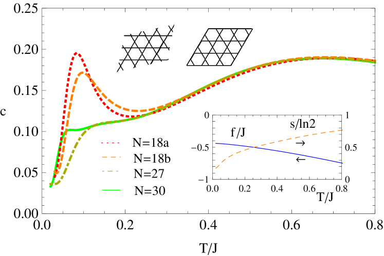
We also estimate the error caused from the random initial vector by using inequality (15). In the inset of Fig. 1 we plot (left scale), which are calculated from Eq. (7). Using the results for and those for , we find that the (normalized) standard deviation for is less than % down to . The error of itself is also estimated to be less than % down to . Such a small error is attained because our method gets more accurate for larger entropy and the KHA has relatively large at low temperature due to the frustration effect Sindzingre . To see this quantitatively for , we plot in the inset of Fig. 1 (right scale). At there remains % of the total entropy (). Such a large entropy makes small.
Finally, to confirm the validity, we compute for , for which the result of the ND is available N18 . For such a small cluster, the standard deviation estimated from inequality (15) is about % at . Hence, we have used Eq. (2) for only, taking average over realizations of the TPQ state. The difference between our results (a, b) and those by the ND N18 is less than the line width of the data in Fig. 1.
Acknowledgements.
We thank K. Asano, C. Hotta, K. Hukushima and H. Tasaki for helpful discussions. This work was supported by KAKENHI Nos. 22540407 and 23104707. SS is supported by JSPS Research Fellowship No. 245328.References
- (1) S. Popescu, A.J. Short, and A. Winter, Nature Phys. 2, 754 (2006).
- (2) S. Goldstein et al, Phys. Rev. Lett. 96, 050403 (2006).
- (3) A. Sugita, RIMS Kokyuroku (Kyoto) 1507, 147 (2006) [in Japanese].
- (4) A. Sugita, Nonlinear Phenom. Complex Syst. 10, 192 (2007).
- (5) P. Reimann, Phys. Rev. Lett. 99, 160404 (2007).
- (6) S. Sugiura and A. Shimizu, Phys. Rev. Lett. 108, 240401 (2012).
- (7) The Hilbert space of any quantum system is separable, in the irreducible representation. That is, its basis vectors are countable even when its dimension is infinite as in particle systems. Furthermore, one can take the basis vectors in such a way that increases with increasing . When the energy scale of interest is (), one can truncate the basis to , where (and ). One thus obtains an effective Hilbert space of finite dimension . Note however that Eqs. (1)-(7) hold even when .
- (8) For , denotes that such that for all .
- (9) H. B. Callen, Thermodynamics (John Wiley and Sons, New York, 1960).
- (10) A. Shimizu, Netsurikigaku no Kiso (Principles of Thermodynamics) (University of Tokyo Press, Tokyo, 2007) [in Japanese].
- (11) W. Thirring, Z. Physik 235, 339 (1970).
- (12) N. Ullah, Nucl. Phys. 58, 65 (1964).
- (13) See Supplemental Material at http://as2.c.u-tokyo.ac.jp/archive/Supplymentary_canonicalTPQ.pdf for the detailed derivations and discussions.
- (14) Although mechanical variables can also be obtained from , formula (4) is often more convenient for them.
- (15) We can also obtain better formulas by replacing in Eq. (9) with or of Ref. SS2012 .
- (16) A. Shimizu and T. Miyadera, Phys. Rev. Lett. 89, 270403 (2002).
- (17) A. Sugita and A. Shimizu, J. Phys. Soc. Jpn. 74, 1883 (2005).
- (18) A. Shimizu, J. Phys. Soc. Jpn. 77, 104001 (2008).
- (19) V. Elser, Phys. Rev. Lett. 62, 2405 (1989).
- (20) N. Elstner and A. P. Young, Phys. Rev. B 50, 6871 (1994).
- (21) P. Sindzingre, G. Misguich, C. Lhuillier, B. Bernu, L. Pierre, Ch. Waldtmann, and H.-U. Everts, Phys. Rev. Lett. 84, 2953 (2000).
- (22) M. Isoda, H. Nakano, and T. Sakai, J. Phys. Soc. Jpn 80, 084704 (2011).