Connectivity driven Coherence in Complex Networks

Abstract

We study the emergence of coherence in complex networks of mutually coupled non-identical elements. We uncover the precise dependence of the dynamical coherence on the network connectivity, on the isolated dynamics of the elements and the coupling function. These findings predict that in random graphs, the enhancement of coherence is proportional to the mean degree. In locally connected networks, coherence is no longer controlled by the mean degree, but rather on how the mean degree scales with the network size. In these networks, even when the coherence is absent, adding a fraction $s$ of random connections leads to an enhancement of coherence proportional to $s$. Our results provide a way to control the emergent properties by the manipulation of the dynamics of the elements and the network connectivity.

Among the large variety of dynamical phenomena observed in complex networks, collective behavior is ubiquitous and has proven to be essential to the network function Fries ; PS ; Tiago ; Attention ; Singer ; Ep ; Gorka ; Kurths . During the last decades, our understanding of collective behavior of complex networks has increased significantly. Most research focuses on synchronization of diffusively coupled of periodic elements with distinct frequencies Strogatz1 ; Strogatz ; Bernard and identical chaotic elements Pecora2 ; Wu .

In nature the interacting elements in complex networks are non-identical, in such situations complete synchronization is no longer possible, but a highly coherent state can be observed. Examples include collections of coupled maps Ott , power grid networks Kurths , superconducting Joseph junctions Strogatz1 , and brain networks Attention ; Singer ; Ep ; Gorka . In these systems, coherence is characterized by the mean field controlling the behavior of the nodes. Of major importance is how the coherence properties of a general collection of non-identical nodes depends on the structural parameters of the network, on the coupling function, and on the node dynamics. Recent work has elucidated how the dynamics of the nodes can influence coherence in terms of mean field approximations for coupled maps Ott , construction of a Lyapunov function Hasler , and extending the Lyapunov exponents approach Bollt ; Hill . Moreover, control techniques have also been used Qiang ; Cai . Although, this problem has received increasing attention, the effect of network connectivity on the coherent systemic behavior still remains elusive.

In this letter, we uncover how the dynamical coherence of the network depends on the node dynamics, the coupling function, and the network connectivity. Our approach is fully analytical and holds for a class of interaction functions whose Jacobian has positive real part spectrum. We find that in purely random networks, coherence is controlled by the mean degree. In locally connected networks, the mean degree no longer determines coherence, instead coherence is determined by an interplay between the network size and the degree of the nodes. If the mean degree scales properly with the network size, coherence emerges as the network grows. In these networks, even if coherence is absent, by adding random connections we can induce coherence.

The dynamics of a network of $n$ coupled elements with interaction akin to diffusion is described by

$$\frac{d\bm{x}_{i}}{dt}=\bm{f}_{i}(\bm{x}_{i})+\alpha\sum_{j}A_{ij}\bm{H}(\bm{x}_{j}-\bm{x}_{i}),$$ (1)

where $\bm{f}_{i}:\mathbb{R}^{m}\rightarrow\mathbb{R}^{m}$ is smooth and governs the dynamics of the isolated nodes. $\bm{H}:\mathbb{R}^{m}\rightarrow\mathbb{R}^{m}$ is a smooth coupling function, $\alpha$ is the overall coupling strength, $A_{ij}=1$ if nodes $i$ and $j$ are connected and $A_{ij}=0$ otherwise. The degree, that is, the number of connections, of the $i$th node is given by $k_{i}=\sum_{j}A_{ij}$. In this model, coherence is related to the Laplacian $\bm{L}$ where $L_{ij}=\delta_{ij}k_{i}-A_{ij}$ and $\delta_{ij}$ is the Kronecker delta symbol.

We assume that the coupling function possesses the following properties: $i)$ $\bm{H}(\bm{0})=\bm{0}$, $ii)$ the Jacobian of the coupling function $D\bm{H}(\bm{0})=\bm{\Gamma}$ has spectrum on the right part of the complex plane. Throughout the paper, $\beta>0$ denotes the smallest real part of the eigenvalues of $\bm{\Gamma}$. The hypothesis on the spectrum of the Jacobian guarantees the stability of the problem, and cannot be omitted, otherwise, instabilities could appear due to an interplay between the dynamics of the individual nodes and the coupling function. Here, the norm $\|\cdot\|$ denotes the Euclidean norm.

Main result: We consider $\bm{f}_{i}=\bm{f}+\bm{p}_{i}$, where $\|\bm{p}_{i}\|\leq\delta$ uniformly for all nodes Unif . We call $\delta$ the heterogeneity parameter. Our main finding is that, for large times, fluctuations of the trajectories are bounded by

$$\|\bm{x}_{i}(t)-\bm{x}_{j}(t)\|\leq\frac{K\delta}{\alpha\beta\lambda_{2}-\alpha_{c}}$$ (2)

where $\delta$ measures the heterogeneity among the node dynamics, $K=K(\bm{\Gamma})$ is a constant, $\alpha$ is the interaction strength, $\alpha_{c}=\alpha_{c}(\bm{f},\bm{H})$ is positive if the isolated dynamics is chaotic, otherwise $\alpha_{c}=0$, and $\lambda_{2}=\lambda_{2}(\bm{L})$ is the spectral gap, i.e., the second smallest eigenvalue of the Laplacian matrix $\bm{L}$. Roughly speaking, our assumptions will guarantee that the coherence of the set of non-identical nodes is determined by the synchronization properties of the system of identical nodes $\delta=0$.

A network of identical nodes: The situation of zero heterogeneity $\delta=0$ was studied in great detail in the past decades in terms of the master stability function Pecora2 . Here, we develop a theory based on dichotomies Martin , and their persistence. This allows us to develop a complete analytical treatment of the problem. The fully synchronized state $\bm{x}_{1}=\cdots=\bm{x}_{n}$ is invariant under the equation of motion for all values of the coupling strength $\alpha$, and it is called the synchronization manifold. To study the stability we expand the coupling function about the synchronization manifold, which yields $\bm{H}(\bm{x}_{j}-\bm{x}_{i})=\bm{\Gamma}(\bm{x}_{j}-\bm{x}_{i})+\bm{r}(\bm{x}_{j}-\bm{x}_{i}),$ where $\bm{r}$ is a nonlinear Taylor remainder. We use the following convenient notation, denote $\bm{X}=\mbox{col}(\bm{x}_{1},\cdots,\bm{x}_{n}),$ here col stands for the vector formed by stacking the column vectors $\bm{x}_{i}$ into a single column vector, note that $\bm{X}\in\mathbb{R}^{nm}$. Similarly $\bm{F}(\bm{X})=\mbox{col}(\bm{f}(\bm{x}_{1}),\cdots,\bm{f}(\bm{x}_{n})).$ Let $\otimes$ denote the tensor product. The dynamics of a network of identical nodes can be represented in tensor form as $\bm{X}^{\prime}=\bm{F}(\bm{X})-\alpha(\bm{L}\otimes\bm{\Gamma})\bm{X}+\bm{R}_{H}$, where $\bm{R}_{H}$ is the Taylor remainder of the coupling function.

The vector $\bm{1}=(1,1,\cdots,1)/\sqrt{n}$, is an eigenvector of the Laplacian associated with the zero eigenvalue. Moreover, since the eigenvectors of $\bm{L}$ are orthogonal, we consider the following decomposition $\bm{X}=\bm{1}\otimes\bm{s}+\bm{\xi}$, where $\bm{\xi}$ does not lie in the span of $\bm{1}\otimes\bm{s}$. Note that if $\bm{\xi}$ is zero, then the system is fully synchronized. The variational equation governing the $\bm{\xi}$ reads as $\bm{\xi}^{\prime}=\bm{K}(t)\bm{\xi}$, with $\bm{K}(t)=\bm{I}_{n}\otimes D\bm{f}(\bm{s}(t))-\alpha\bm{L}\otimes\bm{\Gamma}$, where we neglected the nonlinear terms. The unique solution of this equation can be represented in terms of the evolution operator $\bm{\xi}(t)=\bm{T}(t,s)\bm{\xi}(s)$. We postpone technical manipulations Longer_version and present the main result concerning the contraction properties of the evolution operator $\|\bm{T}(t,s)\|\leq K\exp\{-[\alpha\beta\lambda_{2}-\alpha_{c}](t-s)\}$ for any $t\geq s$, where $K=K(\bm{\Gamma})$ is a constant independent of the network, $\alpha$ is the coupling strength, $\beta>0$ is the smallest eigenvalue of $\bm{\Gamma}$, and $\lambda_{2}$ is the spectral gap of the Laplacian. Here, $\alpha_{c}=\alpha_{c}(\bm{f},\bm{H})$, and is positive if the node dynamics $\bm{f}$ has positive Lyapunov exponents. Note that since the contraction of the evolution operator is uniform the nonlinear remainders will not effect the stability of the transient towards synchronization. This finding implies that starting at a time $s$ with nearby initial conditions we obtain $\|\bm{x}_{j}(t)-\bm{x}_{i}(t)\|\leq Ce^{-(\alpha\beta\lambda_{2}-\alpha_{c})(t-s)}.$ for all $t\geq s$. Therefore, the characteristic decay time is $1/[\alpha\beta\lambda_{2}-\alpha_{c}]$. Next, we show that the characteristic time controls the coherence of the heterogeneous network.

Effect of the Heterogeneity: We consider Eq. (1) with node dependent maps $\bm{f}_{i}$. Again, we represent the equations in the tensor representation, and perform the same decomposition as before $\bm{X}=\bm{1}\otimes\bm{s}+\bm{\xi}$. The equation of motion can now be written as $\bm{X}^{\prime}=\bm{F}(\bm{X})-\alpha(\bm{L}\otimes\bm{\Gamma})\bm{X}+\bm{P}(\bm{X})+\bm{R}_{H}(\bm{\xi})$, $\bm{P}=$ col $(\bm{p}_{1},\cdots,\bm{p}_{n})$. We project the equation onto the synchronization manifold and to the orthogonal complement. The first projection gives us an equation for $\bm{1}\otimes\bm{s}$ and the second an equation for perturbations $\bm{\xi}$. After some manipulations, the equation for the perturbations reads $\bm{\xi}^{\prime}=\bm{K}(t)\bm{\xi}+\bm{G}(\bm{X})$, where $\bm{G}(\bm{X})$ is the projection of $\bm{P}$, $\bm{R}_{H}$ and $\bm{R}_{F}$ onto the orthogonal complement of the synchronization manifold. Here, $\bm{R}_{F}$ is the Taylor remainder of the vector field $\bm{F}$ about the synchronization manifold. By the method of variation of parameters the solution becomes $\bm{\xi}(t)=\bm{T}(t,0)\bm{\xi}(0)+\int_{0}^{t}\bm{T}(t,u)\bm{G}(\bm{X}(u))du.$ Then, using the bounds on the norm of the evolution operator together with the triangle inequality for large times we obtain Eq. (2) follows.

We use Eq. (2) to study the effect of network connectivity. To this end, we measure the macroscopic coherence in the network by introducing the quantity

$$E(t)=1-\frac{\sum_{i,j}\|\bm{x}_{i}(t)-\bm{x}_{j}(t)\|}{n(n-1)V},$$ (3)

which quantifies coherence as a measure of the distance between the trajectories of the nodes per link. In Eq. (3), $V$ is a normalization factor $V=\max\|\bm{x}_{i}-\bm{x}_{j}\|$ for $\alpha=0$ (when there is no interaction). If the nodes are uncorrelated then $E\rightarrow 0$, the more coherent the system is $\|\bm{x}_{i}-\bm{x}_{j}\|$ approaches zero, and $E(t)\rightarrow 1$. Hence, when the mean field dominates the dynamics of the individual nodes, we obtain $|1-E(t)|\propto\delta/(\alpha\beta\lambda_{2}-\alpha_{c}).$ The denominator must be positive, so if $\alpha_{c}>0$ and $\lambda_{2}\rightarrow 0$ as $n\rightarrow\infty$, we can loose coherence at a finite network size. To illustrate these findings, we show that in a $2k$ nearest neighbor network there is a critical number of neighbors as a function of the network size $n$ for the transition to coherence.

For concreteness, we explore these findings using the Lorenz equation exhibiting a chaotic dynamics Viana to represent the node dynamics. Using the notation $\bm{x}_{i}=(x_{i},y_{i},z_{i})^{*}$, where ^∗ denotes the transpose, the vector field reads $\bm{f}(\bm{x})=(\sigma(y-x),x(r-z)-y,-bz+xy)^{*},$ we choose the classical parameter values $\sigma=10,r=28,b=8/3$. We consider the non-identical behavior as a mismatch in the parameter $\sigma$. Hence, each Lorenz system has $\sigma_{i}=\sigma+\zeta_{i}$, where $\zeta_{i}$ is a random number picked independently according to a uniform distribution with support $[-\varepsilon,\varepsilon]$, yielding $\bm{p}_{i}(\bm{x}_{i})=(\zeta_{i}(y_{i}-x_{i}),0,0)^{*}$. Hence, $\|\bm{p}_{i}(\bm{x}_{i})\|\leq M\varepsilon$, where $M$ is such that $|x-y|<M$, for the Lorenz $M\approx 40$. Note that with this choice the heterogeneity is $\delta=2M\varepsilon$. For simplicity we choose $\bm{H}(\bm{x})=\bm{x}$. We fix the coupling strength $\alpha=10$. The trajectories of the Lorenz accumulate in a neighborhood of a chaotic attractor, and hence, $\alpha_{c}>0$ Alphac . For our numerical simulations, we used the 4th order Runge-Kutta integration scheme with integration step $10^{-4}$.

Locally Connected Networks: Consider a network of $n$ nodes, in which each node is coupled to its $2k$ nearest neighbors. The network Laplacian can be diagonalized and the spectral gap explicitly obtained $\lambda_{2}=2k+1-{\sin[(2k+1)\pi/n]/\sin(\pi/n)}$ Kurths . We analyze $k$ as a function of the network size $n$ as $k=\lceil n^{\gamma}/2\rceil$ – where $\lceil x\rceil$ is the largest integer that approximates $x$. It follows that there exists a critical number of neighbors needed for the network to self organize towards coherence, that is, there is a critical $\gamma_{c}$ such that for $\gamma>\gamma_{c}$ there is a transition to self organization and coherence is enhanced as the network size increases: the heterogeneity is suppressed and the mean field dominates the dynamics. In contrast, for $\gamma<\gamma_{c}$ coherence is absent. The value of $\gamma_{c}$ for onset of coherence can be predicted by analyzing the zero of the denominator of Eq. (2). For $k\ll n$ we obtain, up to the leading order in $n$, the following equation for the critical value of $\gamma_{c}$:

$$\gamma_{c}=\frac{1}{3}\left[2-\frac{\log\left(\frac{\pi^{2}\alpha\beta}{6\alpha_{c}}\right)}{\log n}\right].$$ (4)

We check these predictions against the numerical simulations of the Lorenz dynamics. We consider $\varepsilon=0.2$, and for each fixed system size $n$ considering $k=\lceil n^{\gamma}/2\rceil$, we vary $\gamma$ and measure $E(t)$, see Eq. (3). The value of $\gamma_{c}$ is determined by observing the behavior of $E$. Typically, $E\approx 0$ before the transition to coherence, and after the transition $E\approx 0.97$. Since, the transition from an incoherent to a coherent state is sharp, we can easily detect the value of $\gamma_{c}$. This numerical determination of $\gamma_{c}$ is presented as open circles in Fig. 1, against the theoretical prediction presented as a solid line. Likewise, for a fixed $\gamma$ we can vary the system size and determine the transition in $E$. Again, we find the critical network size as a function of $\gamma$. In the inset a) of Fig. 1, we exhibit a case where we fixed $\gamma=0.3$ and varied the system size. A sharp transition towards loss of coherence can be observed for $n=41$.

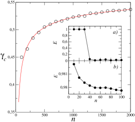
Figure 1: $\gamma_{c}$ as a function of the network size $n$ for $k=\lceil n^{\gamma}/2\rceil$. We fixed $\alpha=10$ and $\varepsilon=0.2$, and recall $\beta=1$. The open circles represent the numerical determination of $\gamma_{c}$, and the solid line is the theoretical prediction, obtained solving $\alpha\beta\lambda_{2}-\alpha_{c}=0$ for $\gamma$. The inset $a)$ shows the critical behavior of $E(t)$ for $\gamma=0.3$ as a function of the network size. Here at the critical network size $n=41$ coherence is lost, agreeing with the theoretical predictions. Inset $b)$ we present the same numerical simulations of the Lotka-Volterra model. As we predict no abrupt transition is observed once $\alpha_{c}=0$.

If the isolated dynamics has $\alpha_{c}=0$, then there is no abrupt transition towards coherence. Either an enhancement of coherence for $\gamma>\gamma_{c}$, or a deterioration for $\gamma<\gamma_{c}$. An example of this situation is observed in the standard Lotka-Volterra model. The state vector $\bm{x}$ of the model is two dimensional, and the vector field reads $\bm{f}(\bm{x})=(x[a-by],y[-d+cx])^{*}$. This system has a constant of motion, which means that $\alpha_{c}=0$. For simplicity we consider all parameters equal to $1$ and mismatches in the parameter $a$ as $a_{i}=a+\zeta_{i}$, which $\zeta_{i}$ as before. In our simulations on $2k$ nearest neighbor network, we fixed $\varepsilon=0.2$, $\gamma=0.3$ and vary the network size $n$. We present the results in the inset $b)$ of Fig. 1. We observed no abrupt transition to loss of coherence, in agreement with our predictions.

Small World graphs: Enhancing Collective Motion. Starting from a nearest neighbor network where no coherence is observed, we can enhance coherence by adding in a small fraction of random links. We add $sn$ edges picked at random from the remaining unconnected pairs, so that the average number of shortcuts per node is $s$. This new network is called small world. A perturbation theory allows to estimate the expected values of the Laplacian spectral gap. Computing the eigenvalues of the Laplacian perturbatively reveals that for ${1/3}<\gamma<1$, also considering $n\gg 1$, we obtain that $\lambda_{2}=2s+O(n^{\gamma-1})$ is the expected value of the eigenvalue. As before, the denominator of Eq. (2) must be positive, and this provides a critical number of shortcuts $s_{c}$ that must be added to obtain coherence. If $s$ is larger then $s_{c}$ we undergo a transition to onset of coherence and, up to high order corrections in the system size, where the coherent measure is given by $|1-E(t)|\propto\delta/s.$ We check this prediction against numerical simulations using the Lorenz dynamics to model the nodes. Starting from the nearest neighbor network of size $n=1000$ and $\gamma=0.3$ (no coherence is observed), we add a fraction of $s$ random edges. We then vary $s$ and measure the coherence. The result can be observed in the inset Fig. 2 $a)$. The theoretical prediction is in excellent agreement with our simulations of the Lorenz dynamics. Thus, by adding a small fraction of random connections we induce coherence. Here, the enhancement of coherence is proportional to the fraction of random shortcuts $s$.

Random Networks: As we discussed in the previous paragraph random structures can enhance coherence. In purely random networks, the coherence is proportional to the mean degree. We use a random graph model $G(\bm{w})$ for a sequence of expected degrees ${\bm{w}}=(w_{1},w_{2},\cdots,w_{n})$. Each element of the adjacency $A_{ij}$’s is an independent Bernoulli variable, taking value $1$ with success probability $p_{ij}=w_{i}w_{j}\rho,$ where $\rho=1/\sum_{i=1}^{n}w_{i}.$ The sequence must satisfy the condition $w_{1}^{2}\leq\rho$ to assure that $p_{ij}\leq 1$. Under these constructions $w_{i}$ is the expected value of $k_{i}$. The mean degree $m=1/(n\rho)$ determines the spectral gap $\lambda_{2}$. The Erdös-Rényi random graphs correspond to the constant case $w_{i}=pn$. If $p$ is constant then the expected value of $\lambda_{2}$ is concentrated at $m$. The power law graphs correspond to the case, $w_{i}\propto i^{-1/(\theta-1)}$, with $\theta\geq 2$. See Ref. CombChung for details on this choice of $w_{i}^{\prime}s$. The parameter $\theta$ characterizes the degree distribution, that is, the probability $P(k)$ to find a degree between $k$ and $k+\Delta k$, behaves as a power law $P(k)\propto k^{-\theta}$. If the network is large, the expected value of the spectral gap $\lambda_{2}$ is concentrated at $m(1-1/(\theta-1))$, see Ref. Wu . In these cases, for large mean degrees $m$, we obtain the scaling $|1-E|\propto\delta/m$.

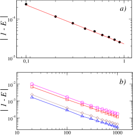
Figure 2: Randomness enhance coherence. In $a)$ Log-Log plot of coherence $|1-E|$ versus the fraction of randomly added links $s$. For fixed $\alpha=10$. starting from a $2k$ nearest neighbor network of size $n=1000$ and $\gamma=0.3$ no coherence is observed. We then add a fraction of $s$ random links. This induces coherence in the network according to $|1-E|\propto s^{-1}$, as predicted theoretically. In $b)$ Log-Log plot of coherence $|1-E|$ versus the mean degree $m$. For $n=3000$, we simulate the Lorenz dynamics on Erdös-Rényi with $\varepsilon=1$ ($\square$), Power law networks with $\theta=3$ and $\varepsilon=1$ ($\circ$). Then with $\varepsilon=0.2$ for $\theta=2.7$ ($\diamond$) and $\theta=4$ ($\bigtriangleup$). The scaling towards coherence $|1-E|\propto\delta/m^{-1}$ agrees with the theoretical prediction.

We constructed these random networks with size $n=3000$ and studied numerically the coherence properties as a function of the mean degree $m$ and heterogeneity $\delta=2M\varepsilon$. Our numerical simulations using the Lorenz dynamics yield $E=1-O(\delta/m)$, in excellent agreement with our predictions, see Fig. 2 b).

In summary, we have uncovered the dependence of network coherence on the dynamics of the nodes, the network connectivity and the coupling function. In random networks, dynamical coherence is enhanced with the increase of the mean degree. These networks exhibit high connectivity. In regular networks the mean degree no longer controls the emergence and enhancement of coherence, rather we encounter a critical behavior: if the mean degree scales properly with the system size coherence emerges. We were able to determine such critical behavior analytically. In our numerical illustrations, we chose the non-identical part $\bm{p}_{i}$ as a mismatch component. Our approach is general and $\bm{p}_{i}$ can be an essentially different system, or a noise driven component. In the later case, our results predict a noise suppression due to network effects. Formula (2) explains how the connectivity can enhance coherence, which can be useful for many applied areas where coherence plays a fundamental role such power grid networks and neuroscience.

We are in debt with A. Pikovsky, R. Vilela, and J. Eldering for illuminating conversations. This work was financially supported by Leverhulme Trust Grant No. RPG-279, CNPq, TUBITAK Grant No. 111T677.

References

- (1) P. Fries, Trends Cogn. Sci. 9, 474 (2005).
- (2) T. Pereira, et al., Phys. Rev. E 75, 026216 (2007).
- (3) T. Pereira, Phys. Rev. E 82, 036201 (2010).
- (4) G.G. Gregoriou et al., Science 324, 1207 (2009).
- (5) W. Singer, Neuron 24, 49 (1999).
- (6) John Milton and Peter Jung (Ed), Epilepsy as a Dynamic Disease, Springer, 2010.
- (7) G. Zamora-Lopez et al., Front. Neurosci. 5, 83 (2011).
- (8) A. Arenas et al., Phys. Rep. 469, 93 (2008).
- (9) K. Wiesenfeld et al., Phys. Rev. Lett. 76, 404 (1996).
- (10) S.H. Strogatz, Physica D 143, 1 (2000).
- (11) B. Sonnenschein et al., Eur. Phys. J. B 86, 12 (2013).
- (12) M. Barahona and L. Pecora, Phys. Rev. Lett. 89, 054101 (2002).
- (13) C.W. Wu, Phys. Lett. A 319, 495 (2003).
- (14) J. G. Restrepo et al., Phys. Rev. Lett. 96, 254103 (2006).
- (15) I. Belykh et al., Chaos 13, 165 (2003).
- (16) J. Sun et al., Europhys. Lett. 85, 60011 (2009).
- (17) J. Zhao, and D.J. Hill, IEEE TCS-I 58, 584 (2011).
- (18) Q. Song et al., Phys. Let. A 374, 544 (2010).
- (19) S. Cai et al., Phys. Lett. A 374, 2539 (2010).
- (20) If we consider the following norm . We also assume for simplicity that the dynamics of each perturbed node lies within a compact set.
- (21) M. Rasmussen, P. Kloeden, Nonautonomous Dynamical Systems, M. Surv. Mon. 176, AMS (2011).
- (22) T. Pereira et al., arXiv:1304.7679 [math.DS].
- (23) M. Viana, Math. Intel. 22, 6 (2000).
- (24) Our analysis provides an estimate for , this bounds is not sharp. Hence, we use the bounds from the theory of the Lyapunov exponents. However, we could loose coherence due to bubbling. Statistically, these scenarios occur with small probability. Therefore, , and average our numerical experiments over many trials.
- (25) Chung F., Lu L. and Vu V., Annals. Comb. 7, 21 (2003).