Rapid Variability: What do we learn from correlated mm-/gamma-ray variability in jets ?

Abstract:

Densely time sampled multi-frequency flux measurements of the extreme BL Lac object S5 0716+714 over the past three years allow us to study its broad-band variability, and the detailed underlying physics, with emphasis on the location and size of the emitting regions and the evolution with time. We study the characteristics of some prominent mm-/$\gamma$-ray flares in the context of the shock-in-jet model and investigate the location of the high energy emission region. The rapid rise and decay of the radio flares is in agreement with the formation of a shock and its evolution, if a geometrical variation is included in addition to intrinsic variations of the source. We find evidence for a correlation between flux variations at $\gamma$-ray and radio frequencies. A two month time-delay between $\gamma$-ray and radio flares indicates a non-cospatial origin of $\gamma$-rays and radio flux variations in S5 0716+714.

1 Introduction

Blazars constitute a unique laboratory to probe jet formation and its relation to radio-to-$\gamma$-ray variability. The current understanding implies that relativistic shocks propagating down the jet provide a good description of a variety of observed phenomena in AGNs. To provide a framework for the observed flux variations, we tested the evolution of radio flares in context of the standard shock-in-jet model [1; 2]. A shock induced flare follows a particular trend in the turnover frequency – turnover flux density ($S_{m}$ – $\nu_{m}$) diagram. The typical evolution of a flare in the $S_{m}$ – $\nu_{m}$ plane can be obtained by inspecting the $R$ (radius of jet)-dependence of the turnover frequency, $\nu_{m}$ and the turnover flux density, $S_{m}$ [see 3 for details]. During the first stage, Compton losses are dominant and $\nu_{m}$ decreases with increasing radius, $R$, while $S_{m}$ increases. In the second stage, where synchrotron losses are the dominating energy loss mechanism, $\nu_{m}$ continues to decrease while $S_{m}$ remains almost constant. Both $S_{m}$ and $\nu_{m}$ decrease in the final, adiabatic stage. As a consequence, the $S_{m}$ – $\nu_{m}$ diagram is a useful tool to explore the dominance of emission mechanisms during various phases of evolution of a flare.

We report here a radio to $\gamma$-ray variability study of the BL Lac object S5 0716+714. We tested the evolution of radio (cm and mm) flares in context of the standard shock-in-jet model following the $S_{m}$ – $\nu_{m}$ diagram as discussed above. We also investigate the correlation of $\gamma$-ray activity with the emission at lower frequencies, focusing on the individual flares observed between August 2008 and January 2011.

2 Multi-frequency light curves

A broadband flux monitoring of S5 0716+714 was performed over a time period between April 2007 to January 2011. The multi-frequency observations comprise GeV monitoring by Fermi/LAT and radio monitoring by several ground based telescopes. The details of observations and data reduction can be found in [4]. Fig. 1 shows the $\gamma$-ray and radio frequency light curves of the source. The top of the figure shows the weekly averaged $\gamma$-ray light curve integrated over the energy range 100 MeV to 300 GeV. The radio frequency light curves are shown in the bottom of the figure. The source exhibits significant flux variability both at $\gamma$-rays and radio frequencies. Apparently, the two major radio flares (labeled as “R6” and “R8”) are observed after the major $\gamma$-ray flares.

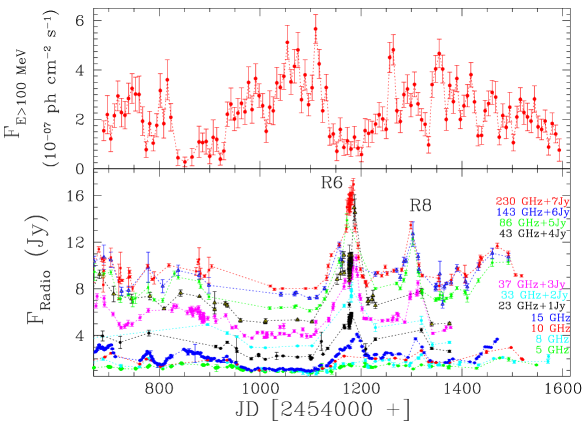
Figure 1: Top : GeV light curve of S5 0716+714 during the first $\sim$3 years of the Fermi/LAT observations from 2008 August to 2011 January at E $>$ 100 MeV. Bottom : Radio frequency light curves of S5 0716+714 observed over the past $\sim$3 years. For clarity, the light curves at different frequencies are shown with arbitrary offsets (indicated by a ”Frequency + x Jy” label). The major radio flares are labeled as ”R6” and ”R8”.

3 Evolution of radio flares in the shock-in-jet scenario

In order to test the evolution of the two major radio flares in the context of a shock-in-jet model, we construct the quasi-simultaneous radio spectra over different time bins as shown in Fig. 2 (a) [see 4 for details] using 2.7 to 230 GHz data. The observed radio spectrum is usually the superposition of emission from the two components : (i) a steady state (unperturbed region), and (ii) a flaring component resulting from the perturbed (shocked) regions of the jet. The quiescent spectrum (Fig. 2 (b) (dotted curve)) is approximated using the lowest flux level during the course of our observations. The quiescent spectrum is described by a power law $F(\nu)=C_{q}(\nu/{\rm GHz})^{\alpha_{q}}$ with $C_{q}=(0.92\pm 0.02)$ Jy and $\alpha_{q}=-(0.06\pm 0.01)$. We subtract the contribution of the steady-state emission from the entire spectrum before modeling.

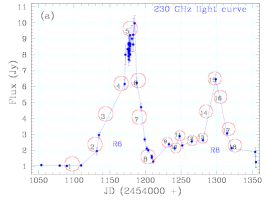
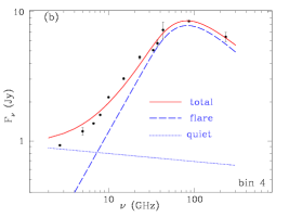
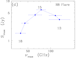
Figure 2: The evolution of the radio spectra: (a) 230 GHz light curve showing different periods over which the spectra are constructed. (b) Results of a single component spectral fitting at time bin “4”, the dotted line corresponds to the quiescent spectrum, the dashed one to the flaring spectrum and the solid line to the total spectrum. (c) $\&$ (d) The time evolution of $S_{max}$ vs $\nu_{max}$ for the R6 and R8 radio flares (see text for details).

We fitted the flare component spectrum using a synchrotron self-absorbed model, which can be described as [see 3; 6 for details] :

$$S_{\nu}=S_{m}\left(\frac{\nu}{\nu_{m}}\right)^{\alpha_{t}}\frac{1-\exp{\left(-\tau_{m}\left(\nu/\nu_{m}\right)^{\alpha_{0}-\alpha_{t}}\right)}}{1-\exp{(-\tau_{m})}},$$ (1)

where $\tau_{m}\approx 3/2\left(\sqrt{1-\frac{8\alpha_{0}}{3\alpha_{t}}}-1\right)$ is the optical depth at the turnover frequency, $S_{m}$ is the turnover flux density, $\nu_{m}$ is the turnover frequency and $\alpha_{t}$ and $\alpha_{0}$ are the spectral indices for the optically thick and optically thin parts of the spectrum, respectively ($S\sim\nu^{\alpha}$).

The evolution of both R6 and R8 flares in the $S_{m}$ – $\nu_{m}$ plane is shown in Fig. 2 (c) – (d). In the standard shock-in-jet model, $S_{m}\propto\nu_{m}^{\epsilon_{i}}$ where $\epsilon_{i}$ depends upon the variation of physical quantities i.e., magnetic field (B), Doppler factor ($\delta$) and energy of relativistic electrons [see e.g. 1;3 for details]. The estimated $\epsilon_{i}$ values are given in Table 1.

Table 1: Different states of spectral evolution and their characteristics

Flare	Time	bin	$\epsilon_{Calculated}$	$\epsilon_{Expected}$	b	Stage
	JD [2454000+]				s=2.2, a=1-2
R6	1096-1178	1-4	-7$\pm$3	-2.5	0.7	Compton
	1178-1194	4-5	0	0	-0.07	Synchrotron
	1194-1221	5-8	10$\pm$2	0.7	2.6	Adiabatic
R8	1283-1303	13-15	-0.9$\pm$0.1	-2.5	0.4	Compton
	1298-1345	15-18	1.8$\pm$0.2	0.7	-2	Adiabatic

$\delta\propto R^{b}$, $B\propto R^{-a}$ and $N(\gamma)\propto\gamma^{-s}$

We notice that there is a significant difference between the theoretically expected (from [1]) and our calculated $\epsilon$ values (see Table 1). Therefore, the rapid rise and decay of $S_{m}$ w.r.t. $\nu_{m}$ particularly in the case of the R6 flare (see Fig. 2) rule out these simple assumptions of a constant Doppler factor ($\delta$). Consequently, we consider the evolution of radio flares including dependencies of physical parameters $a$, $s$ and $d$ following (7). Here, $a$, $s$ and $d$ parametrize the variations of $\delta\propto R^{b}$, $B\propto R^{-a}$ and $N(\gamma)\propto\gamma^{-s}$ along the jet radius. Since it is evident that the $\epsilon$ values do not differ much for different choices of $a$ and $s$ [7], we assume for simplicity $s\approx$ constant. For the two extreme values of $a=1$ and 2, we investigate the variations in $b$. The two different $a$ values give similar results for $b$. The calculated values of $b$ for the different stages of evolution of the radio flares are given in Table 1. As a main result, we conclude that the Doppler factor varies significantly along the jet radius during the evolution of the two radio flares.

4 Correlated mm-gamma-ray variability

We apply the discrete cross-correlation function (DCF) [8] analysis method to investigate a possible correlation among flux variations at radio and $\gamma$-ray frequencies. In Fig. 3, we report the DCF analysis results of the weekly averaged $\gamma$-ray light curve with the 230 GHz radio data. To estimate the possible peak DCF value and respective time lag, we fit a Gaussian function to the DCF curve with a bin size of 11 days. The Gaussian function has a form: $DCF(t)=a\times~{}exp[\frac{-(t-b)^{2}}{2c^{2}}]$, where $a$ is the peak value of the DCF, $b$ is the time lag at which the DCF peaks and $c$ characterizes the width of the Gaussian function. The best-fit function is shown in Fig. 3 and the fit parameters are $a=0.94\pm 0.30$, $b=(67\pm 3)$ days and $c=(7\pm 2)$ days. The significance of the correlation is checked using the linear Pearson correlation method which gives a confidence level $>$97$\%$. This indicates a clear correlation between the $\gamma$-ray and 230 GHz radio light curves of the source with the GeV flare leading the radio flare by $(67\pm 3)$ days. Consequently, the flux variations at $\gamma$-rays lead those at radio frequencies $\sim$1 month time period, which suggests a non-cospatial origin of radio and $\gamma$-ray emission in the sense that $\gamma$-rays are produced closer to the central black hole.

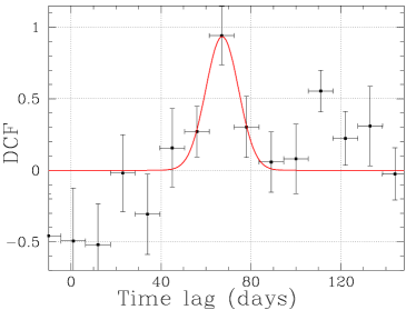
Figure 3: Discrete cross-correlation function (DCF) of the $\gamma$-ray light curve w.r.t. the 230 GHz radio light curve. The solid curve is the best fitted Gaussian function to the DCF curve binned at 11 days.

5 Summary and Conclusions

The evolution of the two major radio flares in the $\nu_{m}-S_{m}$ plane shows a very steep rise and decay over the Compton and adiabatic stages with a slope too steep to be explained from intrinsic variations, requiring an additional Doppler factor variation along the jet. For the two flares, we notice that $\delta$ changes as $R^{0.7}$ during the rise and as $R^{2.6}$ during the decay of the R6 flare. The evolution of the R8 flare is governed by $\delta\propto R^{0.4}$ during the rising phase and $\delta\propto R^{-2.0}$ during the decay phase of the flare. Such a change in $\delta$ can be due to either a viewing angle ($\theta$) variation or a change of the bulk Lorentz factor ($\Gamma$) or by a combination of both. The change in $\delta$ can be easily interpreted as a few degree variation in $\theta$, while it requires a noticeable change of the bulk Lorentz factor. A similar behavior has also been observed in a parsec-scale VLBI kinematic study of the source, which showed that the jet components exhibited significantly non-radial motion with regard to their position angle and in a direction perpendicular to the major axis of the jet [9]. Consequently, a correlation between the long-term radio flux-density variability and the position angle evolution of a jet component, implied a significant geometric contribution to the origin of the long-term variability. This can be probably a result of precession at the base of the jet, which leads to twisted and/or helical structures. More observations and modeling is required to understand the physical origin of these phenomena. A formal cross-correlation between flux variations at radio and $\gamma$-ray frequencies suggests that $\gamma$-ray are produced closer to the black hole. The agreement of shock-induced evolution of radio flares with a clear correlation between radio and $\gamma$-rays is a hint for the shock-induced origin of $\gamma$-ray emission in the source.

Acknowledgments. The $Fermi$ LAT Collaboration acknowledges support from a number of agencies and institutes for both development and the operation of the LAT as well as scientific data analysis. These include NASA and DOE in the United States, CEA/Irfu and IN2P3/CNRS in France, ASI and INFN in Italy, MEXT, KEK, and JAXA in Japan, and the K. A. Wallenberg Foundation, the Swedish Research Council and the National Space Board in Sweden. Additional support from INAF in Italy and CNES in France for science analysis during the operations phase is also gratefully acknowledged. We would like to thank Marcello Giroletti and Stefanie Komossa for their useful comments and suggestions.

References

- (1) A. P. Marscher and W. K. Gear, Models for high-frequency radio outbursts in extragalactic sources, with application to the early 1983 millimeter-to-infrared flare of 3C 273, ApJ 298 (Nov., 1985) 114–127.
- (2) E. Valtaoja, H. Terasranta, S. Urpo, N. S. Nesterov, M. Lainela, and M. Valtonen, Five Years Monitoring of Extragalactic Radio Sources - Part Three - Generalized Shock Models and the Dependence of Variability on Frequency, A&A 254 (Feb., 1992) 71.
- (3) C. M. Fromm, M. Perucho, E. Ros, T. Savolainen, A. P. Lobanov, J. A. Zensus, M. F. Aller, H. D. Aller, M. A. Gurwell, and A. Lähteenmäki, Catching the radio flare in CTA 102. I. Light curve analysis, A&A 531 (July, 2011) A95+.
- (4) B. Rani, T. P. Krichbaum, L. Fuhrmann, et al., Radio to gamma-ray variability study of blazar S5 0716+714, A&A accepted (2013), ArXiv e-prints arXiv:1301.7087.
- (5) B. Lott, L. Escande, S. Larsson, and J. Ballet, An adaptive-binning method for generating constant-uncertainty/constant-significance light curves with Fermi-LAT data, A&A 544 (Aug., 2012) A6.
- (6) M. Türler, T. J.-L. Courvoisier, and S. Paltani, Modelling 20 years of synchrotron flaring in the jet of 3C 273, A&A 361 (Sept., 2000) 850–862.
- (7) A. P. Lobanov and J. A. Zensus, Spectral Evolution of the Parsec-Scale Jet in the Quasar 3C 345, ApJ 521 (Aug., 1999) 509–525.
- (8) R. A. Edelson and J. H. Krolik, The discrete correlation function - A new method for analyzing unevenly sampled variability data, ApJ 333 (Oct., 1988) 646–659.
- Britzen et al. (2009) Britzen, S., Kam, V. A., Witzel, A., Agudo, I., Aller, M. F., Aller, H. D., Karouzos, M., Eckart, A., Zensus, J. A. Non-radial motion in the TeV blazar S5 0716+714. The pc-scale kinematics of a BL Lacertae object, A&A 508 (Oct., 2009) 1205–1215.