Searching and Bargaining with Middlemen

Abstract

We study decentralized markets with the presence of middlemen, modeled by a non-cooperative bargaining game in trading networks. Our goal is to investigate how the network structure of the market and the role of middlemen influence the market’s efficiency and fairness. We introduce the concept of limit stationary equilibrium in a general trading network and use it to analyze how competition among middlemen is influenced by the network structure, how endogenous delay emerges in trade and how surplus is shared between producers and consumers.

1 Introduction

In most markets trade does not involve just producers and consumers but also one or more middlemen serving as intermediaries. For example, brokers and market makers fill this role in financial markets as do wholesalers and retailers in many manufacturing industries. Classical economic approaches to studying markets, such as competitive equilibrium analysis, largely abstract away the role of such middlemen; a point made in the introduction of Rubinstein and Wolinsky (1987), who attribute this is to a lack of modeling how trade occurs and the associated frictions involved. Rubinstein and Wolinsky (1987) offer a solution to this shortcoming by adopting a search theoretic model as in Diamond and Maskin (1979), Mortensen (1982), Diamond (1982). Agents meet pairwise over time and must wait until they meet a suitable partner to trade. The time it takes to find a partner is costly thus introducing a search friction. The role of middlemen is in reducing this friction. Subsequently there has been much work in studying different models of trade (e.g., various non-cooperative bargaining models) and using these to analyze how middlemen influence the formation of prices and the efficiency of trade.

Much of the aforementioned work has focused on models in which all producers and consumers have access to the same middlemen. However, often this is not the case due, for example, to various institutional or physical barriers. One example of this as pointed out by Blume et al. (2009) is in agricultural supply chains of developing countries. In such cases, due to inadequate transportation infrastructure, farmers may only be able to trade in local markets. Such relationships are naturally modeled via a network. Blume et al. (2009) consider such trading networks with a focus on characterizing how network structure effects equilibrium prices set by middlemen which have full information and full bargaining power and so there are no trading frictions. Similar equilibrium questions have also been studied in the supply chain literature (e.g. Nagurney et al. (2002)).

The first line of work described above focuses on modeling trade and its associated frictions, assuming simple trading networks (often with a single middleman). On the other hand, the second line of work focuses on the impact of network structure but does not account for trade frictions. The interaction of both these effects is not well understood. In a more complex network, the search problem facing an agent will depend on her location in the network, and the presence of such frictions will naturally given rise to different equilibria than in models such as Blume et al. (2009).

This paper provides a starting point to bridge this gap: as in Blume et al. (2009) we consider a trading network connecting consumers to producers, but as in Rubinstein and Wolinsky (1987), agents randomly meet over time and engage in non-cooperative bargaining protocols. Thus, our paper provides a general framework that incorporates three important features of markets. First is the underlying network structure: not all pairs of agents can interact in the market. The second is the non-cooperative bargaining setting: no agents have the power to set prices, the prices are formed through a negotiation process. Finally, the third is the search cost: agents discount their payoff if they do not find a proper trading partner or fail to negotiate. The possibility of not finding a proper trading partner is an important additional search cost in our model.

It is well known that such complex models are often intractable. However, by considering large markets and adopting a mean-field approach, we show that this type of model becomes tractable and exhibits many interesting properties. In particular, following Nguyen (2012), we consider a non-cooperative bargaining game in a finite network, and study the agents’ behavior in the limit as the population at each node of the network increases. We introduce a notion of a limit stationary equilibrium, and show that it always exists. We then use this concept to investigate the efficiency of the market, how bargaining with middlemen cause endogenous delay in equilibrium, and how network structure influences competition among middlemen and the share of surplus between producers and consumers. To illustrate these new insights, next we describe three properties exhibited at equilibrium in our model that are qualitatively different from the predictions in the existing literature.

Competition among middlemen

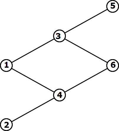
Figure 1: An example trading network with producers (1,2); consumers (5,6) and middlemen (3,4).

First, to illustrate how network structure influences the competition among middlemen, consider the trading network shown in Figure 1. For simplicity, we assume each producer produces a unit of an indivisible good, and each consumer desires one item and obtains a value normalized to 1 dollar upon consuming it. The links in the network represent which pairs of agents can trade and are assumed to be directional links going from left to right. In our model, only pairs of agents that are connected can meet and bargain. Unlike a static model like Blume et al. (2009), we assume agents meet and trade over a infinite, discrete time horizon, where each agent discounts their payoffs by a factor $0<\delta<1$.

In static models without search frictions like Blume et al. (2009), the middleman have all the bargaining power and they simultaneously suggest prices to the producers and consumers for trade to occur. The producers and consumers then use these prices to determine the middlemen they would like to use for the trade. The middlemen never hold the good, and so need not consider the consequences of any future competition between each other. Such models predict that the “bargaining power” of middlemen at nodes 3 and 4 in this network should be the same, because the roles of agents at these nodes can be interchanged if we change the role of producers and consumers. In our model, because of search friction, middlemen do not meet both producers and consumers at the same time and so cannot simultaneously propose prices to each of them. Only after buying a good from producers, can the middlemen resell it to consumers. Assuming this type of market structure significantly changes the outcome. In the network in Figure 1, for example, our results show that there is no symmetry between nodes 3 and 4. In particular, the bargaining power of middlemen at node $3$ is higher than that of a middlemen at node $4$. Middleman $3$ has a competitive advantage on the consumer side: it has access to more consumers than middleman $4$. Thus, when holding a good, middlemen $3$ can find a consumer in an easier and faster manner than $4$. This has an important effect for trade in previous rounds between producers and middlemen. Here, even though $4$ has access to more producers (1 and 2), after buying the good from these producers, middleman 4 is aware that he needs to compete and cannot get as high a surplus as middleman 3, resulting in him not being able to offer good prices to producers 1 and 2. In other words, competition on the consumers’ side has an influence back along the trading network to the competition on the producers’ side, and this disadvantages middleman 4. See Theorem 4.1 for a precise statement.

Endogenous Delay

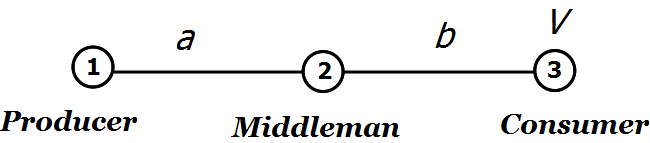
Figure 2: A network exhibiting endogenous delay.

The second distinguishing property of our model is endogenous delay in trade due to the sunk cost problem. Consider the network shown in Figure 2. The producer has to trade with one middleman in order for the good to reach the consumer. Assume that the consumer has a value of $V$ units for consuming the good, and trade on the two links incurs transaction costs of $a$ and $b$ units, respectively.

In an efficient market, if $V>a+b$, so that trade is beneficial, producers would trade with middlemen and middlemen would trade with consumers whenever these agents meet one another. However, in our model, after buying a good from the producer, middlemen needs to bargain with a consumer to resell the good. At this point, the transaction cost $a$ is sunk and is irrelevant in the negotiation. Wong and Wright (2011) consider a model for such a setting, where each node represents a single agent. In such a model, the expected payoff of the middlemen from the re-sale might not be enough to recover the sunk cost, leading to market failure. In our model each node consists of a large population of agents and the “bargaining power” of a middleman agent at location $2$ compared with a consumer agent at location $3$ depends on the competition with other middlemen that are also trying to sell. In particular, if the fraction of middlemen that are selling is small, then when negotiating with consumers, they obtain a higher payoff, which will overcome the sunk cost problem of trading with $1$. However, to maintain the small fraction of middlemen looking to sell, the rate of trades between 1 and 2 needs to be smaller than the rate between 2 and 3. This then implies that when producers and middlemen meet, they do not trade with probability 1. This can only be rationalized if the surplus of trade is the same as the producers’ outside option, which we normalize to be 0. In other words, in this case the producers are indifferent between trading and not trading. When two agents meet, even though they can potentially trade, if they only enact a successful negotiation with a probability $p\in(0,1)$, we interpret this as endogenous delay. This result is formally stated in Theorem 5.2 in Section 5.2.

Contrast with Double Marginalization

Lastly, we contrast the outcome of our model with the classical theory of double marginalization, see for example Lerner (1934) and Tirole (1988). Double marginalization appears in a similar market structure like ours, where producers sell the good to middlemen and middlemen continue to sell to the consumers downstream. The market protocols in these environments, however are different from our model. Namely, in the double marginalization literature, it is assumed that when selling the good producers and middlemen have total market power, and charge a monopoly price to their downstream market. As a consequence, middlemen earn a non-negligible profit, consumers pay higher prices and producers have lower profits.

On the other hand, here we assume no agents have a monopoly market power. The prices are formed through a negotiation process. Furthermore, we assume middlemen are long lived, while producers and consumers exit the game after trading. This captures the contrast between different type of agents: middlemen often stay in the market for a long period, while producers and consumers have limited supply and demand for a certain good and do not participate in the market after getting rid of the supply or having satisfied the demand. This assumption captures many realistic markets among small producers and consumers, who are faced with search problems and need to trade through middlemen; examples of such markets include the following: agricultural markets with farmers, consumers and grocery stores; e-commerce markets with sellers, buyers and entities like Ebay or Amazon; and financial markets involving investors, borrowers and banks.

We will show that these assumptions have a fundamental impact on the price formation in the economy. In particular, as the discount rate goes to 1, so that it does not cost agents to wait, the total equilibrium payoff of producers and consumer approaches the total value of trade. What this means is that as agents are more patient, middlemen earn a negligible fee per transaction. The intuition is that in our model, we assume middlemen stay in the game forever, but do not consume. They instead earn money by flipping the good. Thus, middlemen have an incentive to buy and sell the good relatively fast. On the other hand as the discount rate goes to 1, producers and consumer can engage in costless search and bargaining. This brings down the intermediary fee, and helps the market work more efficiently. Theorem 5.1 states this finding rigorously.

Naturally, when the discount rate is not close to 1, then the above property does not hold. More generally, how the agents share the trade surplus depends on a complex combination of the network structure and the discount rate. We will rigorously study this question in the rest of our paper.

1.1 Related Work

As discussed previously, one line of work that this paper draws upon originates from Rubinstein and Wolinsky (1987) who give a model for search frictions in decentralized trade involving middlemen. The setting in Rubinstein and Wolinsky (1987) can be viewed in terms of our model as a simple three node network, with the nodes corresponding to producers, consumers and middelmen, respectively; trade may occur either directly between a producer and consumer or via a middlemen. As in our model, the market evolves in a sequence of periods, where in each period agents are matched and discount future profits. However, instead of considering a strategic bargaining model as we do, Rubinstein and Wolinsky (1987) consider a model in which if trade is profitable, it occurs with the net surplus being split between the agents. The equilibrium of this market is studied under a steady-state assumption. This is similar to the limit-stationary equilibrium that we consider, except here we show that such a stationary equilibrium emerges naturally in a limiting sense.

The articles Wong and Wright (2011) and Nguyen (2012) extend this type of model to line networks, i.e. networks consisting of a sequence of nodes $v_{1},v_{2},\ldots,v_{m}$ in which trade occurs only between nodes $v_{n}$ and $v_{n+1}$, for $n=1,\ldots,m-1$ (here, $v_{1}$ is a producer, $v_{m}$ a consumer and the remaining nodes are middlemen). Wong and Wright (2011) consider a more extensive bargaining model and study both a model with one agent per node and a model with many agents per node, under a steady-state assumption similar to Rubinstein and Wolinsky (1987). Nguyen (2012) considers a similar bargaining model as in this paper but does not model search friction in the same way. Specifically, in Nguyen (2012) the matching process proceeds by first selecting one agent to be a proposer. The proposer is then always able to find a feasible trading partner if one exists (i.e. if the proposer has a good, it is able to find either a consumer or middleman without the good to trade with). In contrast, in the matching model considered here, a proposing agent may be matched with another agent with whom trade is infeasible, even if a feasible trading partner exists. This increases the search costs and has important consequences. Namely, in Nguyen (2012), it is shown that a limit stationary equilibrium might not exist, while here we show that one always does.

The Rubinstein and Wolinsky (1987) paper and the aforementioned references focus on the role of middlemen in reducing search frictions (see also Yavaş (1994)). Other works have considered a middleman’s role in mitigating information frictions, including Biglaiser (1993), Li (1998); such considerations are not addressed here.

Other related models of decentralized trade in networks include Manea (2011), which considers distributed bargaining in a network consisting of only producers and consumers as well as earlier work including Rubinstein and Wolinsky (1985), Binmore and Herrero (1988), Gale (1987), which consider decentralized bargaining between producer and consumers, where any consumer can potentially trade with any producer without involving any middlemen.

The other line of work this paper draws on is work such as Blume et al. (2009) that focuses on general trading networks and seeks to understand how network structure impacts the division of the gains from trade. As in this paper, Blume et al. (2009) consider general networks with the restriction that all trade must go through a middleman and middlemen do not trade with each other. Here, we also do not consider networks in which middlemen trade with each other, but we do allow for trade routes that do not involve any middlemen. As noted previously, in Blume et al. (2009) middlemen can simultaneously announce prices to buyers and sellers. The full information Nash equilibrium of the resulting pricing game is characterized. Somewhat related equilibria questions have been studied in the context of supply chains (see e.g. Nagurney et al. (2002)), where in this case, producers are able to produce and ship multiple units of a product to middlemen and consumers.

On the technical side, our solution concept of limit stationary equilibria is closely related to work on mean field equilibrium for dynamic games (see e.g. Graham and Méléard (1994), Lasry and Lions (2007), Guéant et al. (2011), Benaim and Boudec (2011)). As in our analysis, the theme in this work is characterizing a notion of equilibria for a “large market,” in which users make decisions based on a steady-state view of the market, where this steady-state view is asymptotically consistent with the user’s actions. In most of the mean field literature, all users are statistically identical, while in our model each user has a fixed type depending on his location in the trading network. This notion is similar to work in Huang et al. (2010), which considers a mean field limit for the control for linear quadratic Gaussian systems where the interaction between users depends on their “locality.”

The remainder of the paper is organized as follows. Section 2 introduces the baseline non-cooperative bargaining model. Section 3 discusses the solution concept of limit stationary equilibrium. Sections 4 and 5 uses this equilibrium to provide comparative analysis of several networks. Section 6 concludes.

2 The Model

In this section we introduce the model that we will use. We start by defining the concept of a trading network.

Trading Network:

We consider a group of producers, consumers and middlemen interconnected by an underlying trading network, which is modeled as a directed graph, $\mathcal{G}=(\mathcal{V},\mathcal{E})$ (see Figure 3). Each node $i\in\mathcal{V}$ represents a population of $N_{i}$ agents, all of which are either consumers, producers or middlemen. Hence, we can partition the set of vertices into the following three disjoint sets: a set of producers denoted by $\mathcal{P}$, a set of middlemen denoted by $\mathcal{M}$, and a set of consumers denoted by $\mathcal{C}$. An agent from the population at a node $i$ will sometime be referred to as a type $i$ agent. Trade occurs over directed edges, i.e., a directed edge $(i,j)\in\mathcal{E}$ indicates that a type $i$ agent can potentially directly trade with any type $j$ agent with the good going from $i$ to $j$ as a result of the trade. With a slight abuse of terminology, we often refer to two such agents as being connected by the edge $(i,j)$. For a consumer to acquire a good from a producer, there must be a (directed) path from the consumer to the producer. If this path has length 1, then the two can directly trade, otherwise they must rely on middlemen to facilitate the trade. For simplicity, we consider networks in which any path between a consumer and producer contains at most one middleman, i.e all such paths are either length 1 or 2. An example of such a network is shown in Figure 3. With this assumption, the set of directed edges, $\mathcal{E}$ can also be partitioned into three disjoint sets: those that directly connect producers to consumers (denoted by $\mathcal{E}_{1}$), those that connect producers to middlemen (denoted by $\mathcal{E}_{2}$), and those that connect middlemen to consumers (denoted by $\mathcal{E}_{3}$).

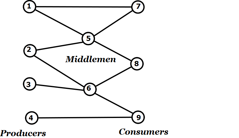
Figure 3: A network among producers, consumers and middlemen.

We assume that there is one type of indivisible good in this economy. All producers produce identical goods and all consumers want to acquire these goods. The value that each consumer of type $c\in\mathcal{C}$ gets from an item is $V_{c}\geq 0$. In every period each agent can hold at most one unit of the good (an item). Thus, in every time period, a middleman either has an item or does not have one. Hence, if there is a directed edge from node $i$ to node $j$, a specific agent of type $i$ can only trade with an agent of type $j$ if the type $i$ agent has a copy of the good and the type $j$ agent does not; we refer to such a pair of agents as feasible trading partners. Note that producers are assumed to always have a good available to trade and consumers are always willing to purchase a good. So, for example, any two agents connected by an edge in the set $\mathcal{E}_{1}$ are always feasible trading partners. For every edge $(i,j)\in\mathcal{E}$, we associate a non-negative transaction cost $C_{ij}\geq 0$; this cost is incurred when trade occurs between an agent at node $i$ and one at node $j$.

Next we discuss the bargaining process that determines the trading patterns for how goods move through the network.

The Bargaining Process:

We consider an infinite horizon, discrete time repeated bargaining game, where agents discount their payoff at rate $0<\delta<1$. Each period has multiple steps and is described as follows.

Step 1. One among all pairs of directly connected nodes $(i,j)\in\mathcal{E}$ is selected at random with a predetermined probability distribution $\pi_{ij})$ on the set of edges $\mathcal{E}$ and one node from each of the corresponding populations is selected uniformly at random. One of these agents is further selected to be a proposer, again chosen at random.

Step 2. If the agents are not feasible trading partners, then the game moves to the next period and restarts at step 1. Recall that this will occur if neither agent has the good or if both have the good.

Step 3. The proposer makes a take-it-or-leave it offer of a price at which he is willing to trade. If the trading partner refuses, the game moves to the next period. Otherwise, the two agents trade: one agent gives the item to and receives the money from the other, and the proposer pays for the transaction cost $C_{ij}$. If a consumer or producer participates in a trade, they exit the game and are replaced by a clone. On the other hand, middlemen are long lived and do not produce nor consume; they earn money by flipping the good.

Step 4. The game moves to the next period, which starts from Step 1.

The game is denoted by $\Gamma(\mathcal{G},\vec{C},\vec{V},\vec{N},{\delta})$, where $\vec{C}$ denotes the vector of links costs, $\vec{V}$ denotes the vector of consumer valuations and $\vec{N}$ denotes the vector of population sizes at each node. Sometimes, we will simply refer to this game as $\Gamma$.

Remarks: We assume middlemen are long lived, on the other hand, producers and consumers exit the game after trading. This captures an extreme contrast between different type of agents: middlemen often stay in the market for a long period, while producers and consumers have limited supply and demand for a certain good. The assumption that we make about the replacement of producers and consumers capture a steady state of an extended economy, where there are incoming flows of producers and consumers at certain rates. Here, to focus on the solution in a steady state, we assume these incoming rates are equal to the rates at which these agents successfully trade. This can be made endogenous as in Gale (1987). However, in a fully endogenous model, a characterization of equilibrium is difficult. Here, we shortcut this problem by assuming the economy is already in a steady state.

In Steps 1 and 2, it is possible that trade is not possible between agents identified at the ends of the chosen link. This leads to additional search friction as it results in a loss of trading opportunity for these two agents. By appropriately choosing the distribution $\pi$ and the choice of proposing agent when trade takes place, we can equivalently view the dynamics from the perspective of the nodes such that the agents are picked independently (following some distribution) to be proposers and depending on the state of the agent (i.e., if the agent possesses the good or not), one among the appropriate edges is chosen following a distribution. Note that even from the node perspective, there is a possibility that the proposing agent might pick an edge along which no trade is possible owing to the picked agent having the same state as the proposing agent; once again, this leads to additional search friction. We prefer to model the dynamics from the perspective of edges as it is more general and fully subsumes the node perspective.

Since we are interested in analyzing the bargaining process defined earlier, as the number of agents in each location increases without bound, we proceed to precisely define the effect of increasing the population size.

Replicated Economy:

Given the bargaining game $\Gamma(\mathcal{G},\vec{C},\vec{V},\vec{N},{\delta})$, the game’s $k$th replication is defined as a game of the same structure except the population size is increased by a factor of $k$ at each node, and the time gap between consecutive periods is reduced by a factor of $T_{k}$. Formally, this is defined as follows:

Definition 2.1

Given the game $\Gamma(\mathcal{G},\vec{C},\vec{V},\vec{N},{\delta})$ and $k,T_{k}\in\mathbb{N}_{+}$, let $\delta^{\prime}=\delta^{1/T_{k}}$. Then the $(k,T_{k})$-replication of $\Gamma$, denoted by $\Gamma^{k}_{T_{k}}(\mathcal{G},\vec{C},\vec{V},\vec{N},{\delta})$ is defined as $\Gamma(\mathcal{G},\vec{C},\vec{V},k\vec{N},\delta^{\prime})$.

Remark: The scaling of the discount rate $\delta$ in this definition is commonly used in the study of dynamical systems. It is clear that without changing $\delta$, in the replicated economy each agent will need to wait for a longer and longer time to get selected, and thus his pay-off approaches $0$. If initially each period takes one unit of time, then note that changing the discount rate to $\delta^{\prime}=\delta^{1/T_{k}}$ is mathematically equivalent to changing the time gap between periods to become $1/T_{k}$ time units and keeping the discount rate fixed. Hence, for example, if we choose $T_{k}=c\cdot k$, it means we keep the rate that each agent sees trading opportunities on the same order as in the original finite game. On the other hand $T_{k}>>k$ models a setting in which the rate at which agents trade is increasing. In this paper, for simplicity, we will focus on the case $T_{k}=k$. Other choices of $T_{k}$ do not affect our results, qualitatively.

3 Solution Concept And Existence Of Equilibrium

Next we turn to the solution concept considered in this paper, that we call a limit stationary equilibrium. To define this equilibrium, we follow Nguyen (2012) and consider the limit of finite agent games as the population increases. In particular, in each game with finite population, we consider a semi-stationary equilibrium in which each agent believes that the economy is already in a steady state and behaves according to a stationary strategy profile. This is certainly not enough. To “close the loop,” a limit stationary equilibrium is defined as a limit of semi-stationary equilibria, whose dynamics converge to the presumed state.

To be more precise, we have the following definitions.

Definition 3.1

The state of the economy is a vector $\vec{\mu}\in[0,1]^{|\mathcal{M}|}$, where $\mu_{m}$ denotes the fraction of middlemen at node $m$ that hold an item.

Definition 3.2

A strategy profile (possibly mixed strategy) is called a stationary strategy if it only depends on an agent’s identity, his state (owning or not owning and item) and the play of the game (which agent he is bargaining with, who the proposer is and what is proposed). More precisely, suppose that agent $i$ and agent $j$ are selected to bargain, and assume $i$ owns an item, $j$ does not, furthermore $i$ is the proposer. In this case, a stationary strategy of agent $i$ is a distribution of proposed prices to agent $j$ and a stationary strategy of agent $j$ is a probability of accepting the offer.

In the rest of the paper, given a stationary strategy, for each link $(i,j)\in\mathcal{E}$ we let $\lambda_{ij}$ denote the conditional probability that $i$ and $j$ trade when they are matched and trade is feasible, that is $i$ owns an item and $j$ does not.

In the following, we first start with the definition of a semi stationary equilibrium in a finite economy, we then use this concept to define limit-stationary equilibria as the size of the economy increases.

3.1 Semi-stationary equilibria

Informally, given a finite game and a state $\vec{\mu}$, a stationary strategy profile is a semi-stationary equilibrium of the game with respect to $\vec{\mu}$, if under the hypothesis that agents believe the state of the economy is always $\vec{\mu}$, no agent can strictly improve his payoffs by changing his strategy.

To define this concept more precisely, we need to introduce the expected pay-offs of agent $i$ depending on whether he possesses or does not possess a good, which we denote by $u_{0}(i)$ and $u_{1}(i)$, respectively. Notice that because of the assumption that producers and consumers exit the market after a successful trade, we have $u_{0}(p)=0$ for all $p\in\mathcal{P}$ and $u_{1}(c)=V_{c}$ for all $c\in\mathcal{C}$. Furthermore, we assume that all agents believe that the state of the economy is captured by $\vec{\mu}$. For the present, we will assume that $\vec{\mu}$ is given. After deriving the incentive conditions depending on $\vec{\mu}$, we will discuss the second type of conditions that give $\vec{\mu}$ endogenously.

The basic structure of the incentive constraints can be captured by the following argument. Assume two agents $i$ and $j$ meet, where $i$ holds the good and $j$ wants it. Also assume that $i$ is the proposer. If the trade is successfully completed, then $j$ possesses the item, thus agent $i$ will demand from agent $j$ the difference of the payoffs between the states before and after the trade (discounted by $\delta$). Note that the state of $i$ also changes, and therefore, if trade is successfully completed, then $i$’s payoff is

$$\delta u_{0}(i)+\delta\big{(}u_{1}(j)-u_{0}(j)\big{)}-C_{ij}.$$

However, agent $i$ has the option of not proposing a trade (or proposing something that will necessarily be rejected by the other party) and earn a payoff of $\delta u_{1}(i)$. Thus, in this situation, the continuation payoff of agent $i$ is

$$\max\{\delta u_{1}(i),\delta u_{0}(i)+\delta\big{(}u_{1}(j)-u_{0}(j)\big{)}-C_{ij}\}.$$

For ease of exposition define the difference between the two terms in this maximization to be

$$z_{ij}:=\delta\Big{(}u_{1}(j)-u_{0}(j)-\big{(}u_{1}(i)-u_{0}(i)\big{)}\Big{)}-C_{ij}.$$ (1)

Thus, the continuation payoff of agent $i$ when he is proposing to $j$ is

$$\delta u_{1}(i)+\max\{z_{ij},0\}.$$

From this we also obtain the following conditions on the dynamics of trade:

1. If $z_{ij}<0$, then agent $i$ will never sell an item to agent $j$ and will wait for a future trade opportunity;

2. If $z_{ij}>0$, then agent $i$ will sell the item to agent $j$ with probability one whenever they are matched; and finally

3. If $z_{ij}=0$, then agent $i$ is indifferent between selling and waiting, thus, the trade can occur with some probability $\lambda_{ij}\in[0,1]$. Conversely, if trade between agents $i$ and $j$ occurs with probability $0<\lambda_{ij}<1$, then we must have $z_{ij}=0$.

Similarly, assume now that instead of $i$, agent $j$ is the proposer, then the continuation payoff of $j$ in this case is $\delta u_{0}(j)+\max\{z_{ij},0\}.$ Furthermore, the same conditions concerning the dynamic of trade between $i$ and $j$, which depends on $z_{ij}$ hold as above, but with the roles of $i$ and $j$ interchanged.

These conditions can be delineated for the general network model introduced in the previous section by considering each type of agent, the state of the agent in terms of holding a good or not, and the probability that he is selected as a proposer. In our model, we have three types of agents: producers, consumers and middlemen. Middlemen are active in the game regardless of having or not having an item. Thus, we will need four types of equations expressing the expected payoff of these agents given their states.

We consider these conditions in detail for the case of producers; the rest follows in similar fashion using the logic outlined earlier. For each producer of type $p\in\mathcal{P}$ who has an item to sell in each period, an agent $p$’s continuation payoff depends on which type of link is selected, the pair of agents that are selected to trade, and whether $p$ is selected as the proposer. Thus, agent $p$’s expected continuation payoff is

$$\sum_{c:(p,c)\in\mathcal{E}_{1}}\frac{\pi_{pc}}{2N_{p}}(\delta u_{1}(p)+\max\{z_{pc},0\})+\sum_{m:(p,m)\in\mathcal{E}_{2}}\frac{\pi_{pm}}{2N_{p}}(1-\mu_{m})(\delta u_{1}(p)+\max\{z_{pm},0\})+$$ (2)

$$+\big{(}1-\sum_{c:(p,c)\in\mathcal{E}_{1}}\frac{\pi_{pc}}{2N_{p}}-\sum_{m:(p,m)\in\mathcal{E}_{2}}\frac{\pi_{pm}}{2N_{p}}(1-\mu_{m})\big{)}\delta u_{1}(p)$$

Here, $z_{pc}$ and $z_{pm}$ are defined as in (1). The first term of (2) represents the case where $p$ is the proposer to a consumer $c$. The second term represents $p$ proposing to a middlemen $m$, who currently does not own a good. Finally, the last term describes the case where $p$ is not a proposer. Here, recall that $N_{p}$ is the size of population at node $p$, and thus, $\frac{\pi_{pc}}{2N_{p}}$, is the probability that the specific agent of type $p$ is the proposer for a consumer $c$. On the other hand, because only a fraction of middlemen are looking to buy, for every middlemen node $m\in\mathcal{M}$, $\frac{\pi_{pm}}{2N_{p}}(1-\mu_{m})$ is the probability that $p$ is matched with $m$, $m$ does not hold a good and $p$ is the proposer. One can interpret this as a form of search friction, that is the probability that a producer can find a trade-able middlemen depends on the state of the economy, which, in turn, impacts the transaction dynamics between the producer and the middleman.

Now, because $\vec{u}$ are assumed to be values of a stationary equilibrium, $u_{1}(p)$ needs to equal the expression in (2). After some algebraic manipulation, this is equivalent to

$$u_{1}(p)=\sum_{c:(p,c)\in\mathcal{E}_{1}}\frac{\pi_{pc}}{2N_{p}(1-\delta)}\max\{z_{pc},0\}+\sum_{m:(p,m)\in\mathcal{E}_{2}}\frac{\pi_{pm}}{2N_{p}(1-\delta)}(1-\mu_{m})\max\{z_{pm},0\}.$$ (3)

Similarly, for the two type of middlemen (either owning an item or not) and the consumers, we have the following set of equations:

$$\forall m\in\mathcal{M}\quad u_{0}(m) =\sum_{p:(p,m)\in\mathcal{E}_{2}}\frac{\pi_{pm}}{2N_{m}(1-\delta)}\max\{z_{pm},0\},$$ (4)

$$\forall m\in\mathcal{M}\quad u_{1}(m) =\sum_{c:(m,c)\in\mathcal{E}_{3}}\frac{\pi_{mc}}{2N_{m}(1-\delta)}\max\{z_{mc},0\},$$ (5)

$$\forall c\in\mathcal{C}\quad u_{0}(c) =\sum_{p:(p,c)\in\mathcal{E}_{1}}\frac{\pi_{pc}}{2N_{c}(1-\delta)}\max\{z_{pc},0\}+\sum_{m:(m,c)\in\mathcal{E}_{3}}\frac{\pi_{mc}}{2N_{c}(1-\delta)}\mu_{m}\max\{z_{mc},0\},$$ (6)

where $z_{pm},z_{mc},z_{pc}$ are defined as

$$z_{ij}=\delta\Big{(}u_{1}(j)-u_{0}(j)-\big{(}u_{1}(i)-u_{0}(i)\big{)}\Big{)}-C_{ij}\;\;\;\forall(i,j)\in\mathcal{E}_{1}\cup\mathcal{E}_{2}\cup\mathcal{E}_{3}.$$ (7)

Once again, the state $\vec{\mu}$ appears in the incentive equations above owing to the particular search model that we consider. As mentioned earlier, since producer and consumers exit the game after trading successfully, we have

$$\forall p\in\mathcal{P}\quad u_{0}(p) =0,$$ (8)

$$\forall c\in\mathcal{C}\quad u_{1}(c) =V_{c}.$$ (9)

We are now ready to define a semi-stationary equilibrium.

Definition 3.3

Given a finite game $\Gamma(\mathcal{G},\vec{C},\vec{V},\vec{N},{\delta})$ and a state $\vec{\mu}$, a stationary strategy profile is a semi-stationary equilibrium with respect to $\vec{\mu}$ if and only if there exists $\vec{u},\vec{z}$ satisfying (3)-(9), and furthermore,

• If $z_{ij}<0$, then irrespective of who the proposer is, agent $i$ will never sell an item to agent $j$, so that he will wait for a future trade opportunity;

• If $z_{ij}>0$, then irrespective of who the proposer is, agent $i$ will sell the item to agent $j$ with probability one whenever they are matched; and finally

• If $z_{ij}=0$, then proposer of the trade is indifferent between trading and waiting. Thus, the trade occurs with some probability $0\leq\lambda_{ij}\leq 1$. In addition, if trade between agents $i$ and $j$ occurs with probability $0<\lambda_{ij}<1$, then $z_{ij}=0$.

3.2 Limit stationary equilibrium

As the economy gets large, we need to consider the behavior of equations (3)-(9), where $N_{i}$ is replaced by $kN_{i}$ and $\delta$ is replaced by $\delta^{1/k}$, as $k$ increases without bound. Note that

$$\lim_{k\rightarrow\infty}k(1-\delta^{1/k})=\ln(1/\delta)\text{ and }\lim_{k\rightarrow\infty}\delta^{1/k}=1.$$

Hence, in the limit, the set of equations (3)-(9) yield the following:

$$\begin{split}\forall p\in\mathcal{P}\quad u_{0}(p)&=0;\\ \quad u_{1}(p)&=\sum_{c:(p,c)\in\mathcal{E}_{1}}\frac{\pi_{pc}}{2N_{p}\ln(1/\delta)}\max\{z_{pc},0\}+\sum_{m:(p,m)\in\mathcal{E}_{2}}\frac{\pi_{pm}}{2N_{p}\ln(1/\delta)}(1-\mu_{m})\max\{z_{pm},0\};\end{split}$$ (10)

$$\forall m\in\mathcal{M}\quad u_{0}(m) =\sum_{p:(p,m)\in\mathcal{E}_{2}}\frac{\pi_{pm}}{2N_{m}\ln(1/\delta)}\max\{z_{pm},0\};$$ (11)

$$\forall m\in\mathcal{M}\quad u_{1}(m) =\sum_{c:(m,c)\in\mathcal{E}_{3}}\frac{\pi_{mc}}{2N_{m}\ln(1/\delta)}\max\{z_{mc},0\};$$ (12)

$$\begin{split}\forall c\in\mathcal{C}\quad u_{0}(c)&=\sum_{p:(p,c)\in\mathcal{E}_{1}}\frac{\pi_{pc}}{2N_{c}\ln(1/\delta)}\max\{z_{pc},0\}+\sum_{m:(m,c)\in\mathcal{E}_{3}}\frac{\pi_{mc}}{2N_{c}\ln(1/\delta)}\mu_{m}\max\{z_{mc},0\};\\ \quad u_{1}(c)&=V_{c};\text{ and}\end{split}$$ (13)

$$z_{ij} =\Big{(}u_{1}(j)-u_{0}(j)-\big{(}u_{1}(i)-u_{0}(i)\big{)}\Big{)}-C_{ij}\;\;\;\forall(i,j)\in\mathcal{E}_{1}\cup\mathcal{E}_{2}\cup\mathcal{E}_{3}.$$ (14)

Using these limiting equations, we now define our solution concept of limit stationary equilibrium. Intuitively, a limit stationary equilibrium is a stationary strategy that can be associated with $\vec{u},\vec{z}$ satisfying (10)-(14) in an similar way to the definition of semi-stationary equilibrium. However, here another condition is added to guarantee that the dynamic given by the stationary strategy will actually converge to the presumed state of the economy $\vec{\mu}$. In particular, recall that a stationary strategy is given by a set of probabilities $\lambda_{ij}$ for every edge $(i,j)\in\mathcal{E}$, which denotes the probability of trade occurring among a pair of feasible trading partners of type $i$ and $j$. If $\lambda_{ij}=1$, trade always occurs and if $\lambda_{ij}=0$ it never occurs. Given any such stationary strategy, the resulting dynamics can be modeled by a Markov process, with the state space being the number of agents at each node holding a good. As the population at each node of the network increases, we want the limit of the stationary distributions of these Markov process to be $\vec{\mu}$. We elaborate on the convergence issue in much greater detail in Section 3.4.

More formally, we have the following definition for a limit stationary equilibrium.

Definition 3.4

Given a finite game $\Gamma(\mathcal{G},\vec{C},\vec{V},\vec{N},{\delta})$ a stationary strategy profile is a limit stationary equilibrium if the stationary distribution of the associated Markov process converges to a point-mass on the state $\vec{\mu}$, and there exists $\vec{u},\vec{z}$ satisfying (10)-(14), moreover

• If $z_{ij}<0$, then irrespective of who the proposer is, agent $i$ will never sell an item to agent $j$, so that he will wait for a future trade opportunity and $\lambda_{ij}=0$;

• If $z_{ij}>0$, then irrespective of who the proposer is, agent $i$ will sell the item to agent $j$ with probability one whenever they’re matched so that $\lambda_{ij}=1$; and finally

• If $z_{ij}=0$, then proposer of the trade is indifferent between trading and waiting. Thus, the trade occurs with some probability $0\leq\lambda_{ij}\leq 1$. In addition, if trade between agents $i$ and $j$ occurs with probability $0<\lambda_{ij}<1$, then $z_{ij}=0$.

3.3 Existence of a Limit stationary equilibrium

We next show that a limit stationary equilibrium always exists.

THEOREM 3.5

For a bargaining game, $\Gamma(\mathcal{G},\vec{C},\vec{V},\vec{N},\delta)$, a limit stationary equilibrium always exists.

Proof: Proof of Theorem 3.5: See Appendix 7.2.

The proof of this theorem is based on a standard fixed-point theorem argument for the best-response correspondences of a fictitious game that is obtained from the incentive constraints and the trading dynamic. The existence of limit stationary equilibria follows as a consequence of the Markov dynamic resulting from our search model, a point that will be elaborated on in the next section. We note, however, that the limit stationary equilibrium might not be unique. In Section 4 we will give a method to compute and check if a stationary strategy is a valid a limit stationary equilibrium.

3.4 Convergence of state of the trading process

As mentioned earlier, one of the key technical lemmas needed to prove the existence of a limit equilibrium is to show that given any stationary strategy profile, the corresponding Markov process in the replicated system will always converge to an unique state, which is also a continuous function of the parameters. This, in return, allows us to define a continuous mapping between two product state-payoff spaces, that can be used in a fixed point argument. In this section, we discuss how to define the state of the trading process and how to determine the $\vec{\mu}$ used for defining both a semi-stationary equilibrium and a limit stationary equilibrium. The formulation of the converging state given our particular Markov process will allow us to compute and construct an equilibrium in various networks in the next section.

We will prove the existence of $\vec{\mu}$ by analyzing the Markov process that drives the state of the system, for a given set of stationary strategies $\{\lambda_{ij}\}$ for $(i,j)\in\mathcal{E}$. Since the state of middlemen can change with time, the entire system can be represented by a vector-valued random process $\{X^{k}_{m}(t):m\in\mathcal{M}\}_{t=1}^{\infty}$ where for the $k^{\mathrm{th}}$ replicated system we keep track of the number of agents who have the item at each middleman type $m\in\mathcal{M}$. For mathematical convenience, we will append $\{X^{k}_{p}(t):p\in\mathcal{P}\}$ where $X^{k}_{p}(t)\equiv kN_{p}$ and $\{X^{k}_{c}(t):c\in\mathcal{C}\}$ where $X^{k}_{c}(t)\equiv 0$ for the states of the producers and the consumers, respectively. Since producers exit the game as soon as they sell their good and are replaced by a clone with a good, at any given time any producer always possesses a good. A similar reasoning holds for the consumers never having a good.

For the $k^{\mathrm{th}}$ replication, the state transitions are given as follows for each $m\in\mathcal{M}$

$$X^{k}_{m}(t+1) =\begin{cases}\min(kN_{m},X^{k}_{m}(t)+1)&\text{w. p. }\rho^{k}_{m}(+1)\\ \max(0,X^{k}_{m}(t)-1)&\text{w. p. }\rho^{k}_{m}(-1)\\ X^{k}_{m}(t)&\text{w. p. }1-\rho^{k}_{m}(+1)-\rho^{k}_{m}(-1),\end{cases}$$

where

$$\rho^{k}_{m}(+1)=\left(1-\frac{X^{k}_{m}(t)}{kN_{m}}\right)\sum_{p\in\mathcal{P}:(p,m)\in\mathcal{E}_{2}}\pi_{pm}\lambda_{pm}$$

is the probability that an agent of type $m$ acquires a good in a given period, and

$$\rho^{k}_{m}(-1)=\frac{X^{k}_{m}(t)}{kN_{m}}\sum_{c\in\mathcal{C}:(m,c)\in\mathcal{E}_{3}}\pi_{mc}\lambda_{mc}$$

is the probability that a type $m$ agent sells a good in a given period. As noted above, the states corresponding to producers in $\mathcal{P}$ and consumers in $\mathcal{C}$ are fixed for all time. This shows that we have a Markov process, and it is easily verified that the process is irreducible.

Since the transition matrix of our Markov process satisfies Lipschitz conditions (see Ethier and Kurtz (2005)), we can analyze the fluid limit that is obtained by scaling time and space, i.e., by considering the process $\{\tilde{X}_{v}^{k}(t):v\in\mathcal{V}\}$, where

$$\tilde{X}_{v}^{k}(t):=\frac{X_{v}^{k}(\lceil kt\rceil)}{k},\qquad\forall v\in\mathcal{V},$$

where $\lceil x\rceil$ for real $x$ is the smallest integer greater than $x$. We will analyze the behavior of the scaled process $\{\tilde{X}_{v}^{k}(t):v\in\mathcal{V}\}_{t\in\mathbb{R}_{+}}$ when $k$ increases without bound. Note that this is the exact scaling considered by the replicated systems discussed earlier. We then have the following result.

Lemma 3.6

Given a set of probabilities for trade $\{\lambda_{ij},(i,j)\in\mathcal{E}\}$, the stationary distribution of the trading dynamic process described above converges to a point-mass on a unique state $\vec{\mu}$, which is the unique solution of

$$\sum_{c\in\mathcal{C}}\pi_{mc}\mu_{m}\left(1-\mu_{c}\right)\lambda_{mc}=\sum_{p\in\mathcal{P}}\pi_{pm}\mu_{p}\left(1-\mu_{m}\right)\lambda_{pm}\quad\forall m\in\mathcal{M},$$ (15)

and which is given by

$$\forall p\in\mathcal{P},\quad\mu_{p} =1;\qquad\qquad\forall c\in\mathcal{C},\quad\mu_{c}=0;$$ (16)

$$\forall m\in\mathcal{M},\quad\mu_{m} =\frac{\sum_{p\in\mathcal{P}:(p,m)\in\mathcal{E}_{2}}\pi_{pm}\lambda_{pm}}{\sum_{p\in\mathcal{P}:(p,m)\in\mathcal{E}_{2}}\pi_{pm}\lambda_{pm}+\sum_{c\in\mathcal{C}:(m,c)\in\mathcal{E}_{3}}\pi_{mc}\lambda_{mc}}.$$ (17)

Proof: Proof of Lemma 3.6: See Appendix 7.1 for details.

For any fixed $k$, the Markov process $\{\tilde{X}_{v}^{k}(t):v\in\mathcal{V}\}$ is irreducible and has finite-states. Therefore, it has a unique stationary distribution. Note that Lemma 3.6 asserts that these stationary distributions converge to a point-mass which is determined by stationary behavior of the limiting process obtained as $m$ increases with bound. In effect, the result above justifies an exchange of the order of limits, $k$ first and time later versus time first and $k$ later. It is both the convergence to a point-mass and this exchange of limits that justifies our definition of semi-stationary equilibria and limit stationary equilibria.

From Lemma 3.6, $\mu_{m}$ for middlemen of type $m$ is the stationary fraction of agents at node $m\in\mathcal{M}$ that hold the good. On the other hand, for the producers we have $\mu_{p}\equiv 1$ for all $p\in\mathcal{P}$ and the consumers we have $\mu_{c}\equiv 0$ for all $c\in\mathcal{C}$. The given values $\{\mu_{m}:m\in\mathcal{M}\}$ satisfy (15), which can be interpreted as a balance condition: for every node $m\in\mathcal{M}$, in every period, the probability that the amount of goods held at node $m$ increases by one or decreases by one should be equal. Looking at this interpretation of (15) more closely, each term on the left-hand-side for a given $c$, $\pi_{mc}\mu_{m}\left(1-\mu_{c}\right)\lambda_{mc}$ is the probability that trade occurs from $m$ to $c$, which requires that link $(m,c)$ is selected (with probability $\pi_{mc}$), that $m$ and $c$ are feasible trading partners (with probability $\mu_{m}(1-\mu_{c})$ so that $m$ has the good and $c$ needs it) and that trade occurs (with probability $\lambda_{mc}$). Similarly, each term on the right-hand-side for a given $p$ can be interpreted as the probability of trade from $p$ to $m$. While the use of $\{\mu_{p}:p\in\mathcal{P}\}$ and $\{\mu_{c}:c\in\mathcal{C}\}$ above is for mathematical convenience, in more general networks (for future work) where we allow middlemen to trade with each other, expressions similar to (15) will hold as the balance condition for every middlemen type where the terms will involve the state of other middlemen as well.

4 Competion Among Middlemen

In this section, we focus on the equilibrium of our model for the network illustrated in Figure 4. For simplicity, we assume all the transaction costs are 0 and each consumer’s valuation of the good is 1. We will analyze the equilibrium as $\delta$ takes values between 0 and 1. Note that $\mathcal{P}=\{1,2\}$, $\mathcal{M}=\{3,4\}$ and $\mathcal{C}=\{5,6\}$.

As discussed in the introduction, because producers at node $1$ have access to more middlemen than at node $2$, producers at $1$ have better bargaining power than producers at $2$. Similarly, consumers at node $6$ are in a better position than consumers at $5$. However, a comparison between the two middlemen position $3$ and $4$ is not straightforward. This is because middlemen at node $3$ have access to consumers at nodes $5$ and $6$, but only one producer node $1$, on the other hand middlemen at node $4$ have access to more producers and fewer consumers.

Figure 4: Transaction costs at every links are 0 and the value for all buyers for obtaining a good is 1.

A precise prediction of the agents’ behaviors depends on the discount rate $\delta$. The factor by which agents discount their payoff if negotiation is not successful also fundamentally influences the trade pattern. In particular, consider trade between 1 and 4. If producers of type $1$ sell to $4$, then they might not be able to get as high a price as compared with selling to middlemen of type $3$, as they are faced with competition from $2$. However, because the opportunity to meet with potential trade partners come randomly, depending on the discount rate, the producers might not have the incentive to wait for a trade opportunity with $3$. Hence, given the network in Figure 1, the pattern of trade depends on both the probability that the agents meet and their discount rate. To make the analysis simple, and to focus on the impact of $\delta$ on the outcome of the market, we assume the population at every node is the same, and the each pair is chosen uniformly at random. We will investigate how changing $\delta$ would influence the trade pattern. In particular, we show that when $\delta$ is small, an equilibrium strategy is for a pair of agents who can trade (that is one has an item to sell, and the other doe not have an item), to trade with probability 1 whenever they meet. However, as agents are more patient ($\delta$ is close to 1), then producers at node 1 never trade with middlemen at node 4. This comparative analysis is summarized in Theorem 4.1.

Before getting to this result, for ease of presentation, we will introduce the following notation:

$$\frac{1}{f(\delta)}:=\frac{\pi_{ij}}{2N_{i}\ln(1/\delta)}.$$

Recall the set of Bellman equations (10)-(14) defining the concept of limit stationary equilibrium where the right hand side of the above equations plays an important role in the qualitative outcome of the game. In the following we will give some comparative analysis based on $f(\delta)$. Notice that when $\delta\rightarrow 1$ , $f(\delta)$ approaches $0$, and when $\delta\rightarrow 0$ , $f(\delta)$ approaches $\infty$.

We call a stationary strategy an always trade strategy, if for every pair of agents that are connected by a link of the network, trade occurs with probability 1, whenever they meet and one agent has an item while the other does not have one. For a link $(i,j)$, a stationary strategy avoids trade on $(i,j)$ if when $i$, and $j$ meet, even though one agent has an item to sell and the other does not have one, they do no trade and rather wait for a future opportunity.

We summarize the comparative analysis studied in this section in the following result.

THEOREM 4.1

The following hold:

• If $f(\delta)=1/2$, then the “always trade” strategy is the unique pure equilibrium, in which case the payoff of middlemen $3$ is greater than that of middlemen $4$.

• If $f(\delta)=1/5$, then the “always trade” strategy cannot be an equilibrium, and the strategy that avoids trade on the link $(1,4)$ and always trades on all other links is the unique pure equilibrium. At this equilibrium too, the payoff of middlemen $3$ is greater than that of middlemen $4$

Remark: Notice that in both cases, payoff of middlemen of type $3$ is greater than that of middlemen of type $4$. As discussed in the introduction, this result is in contrast with models like Blume et al. (2009), where middlemen have all the power to set prices to both producers and consumers simultaneously. In our model, the fact that middlemen need to buy an item first before selling it has important consequences. In particular, middlemen $3$ has an competitive advantage on the consumer’s side: it has access to more consumers than middlemen $4$. Thus, when holding a good, middlemen $3$ can find a consumer easier than $4$. This in return influences trade in the previous round between producers and middlemen. Here even though $4$ has access to more producers ($1$ and $2$), the fact that after buying the good from these producers middleman $4$ is aware that he needs to compete and cannot get as high a surplus as middleman 3, results in him not being able to offer as competitive a price to the producers 1 and 2. In other words, in settings like ours, competition from the consumers’ side is more important because it has an influence back to the competition on the producers’ side.

Theorem 4.1 illustrates another interesting phenomenon about how the discount rate $\delta$ influences the trade pattern. In particular, trade between 1 and 4 only occurs when agents are impatient enough, that is $f(\delta)$ is large. The intuition is similar to the above argument. The advantage of $3$ over $4$ in the consumers’ market influences $4$’s ability to offer good prices to the producers. Thus, when $\delta$ is close to 1, or equivalently $f(\delta)$ is small, a producer of type 1 is better off waiting to trade exclusively with middlemen of type 3. In this case, the advantage that $4$ has over $3$: being connected to both producers nodes disappears, because trade between 1 and 4 will not occur. Clearly in this case, middlemen at node $3$ are in a better position than the middlemen at node 4.

Proof: Proof of Theorem 4.1: The main idea of constructing an equilibrium or showing that a particular strategy is not an equilibrium is as follows.

First, given a strategy, and fixing an $f(\delta)$ value, we calculate the steady state of the economy $\vec{\mu}$ that the replicated Markov process converges to. This step can be calculated as per Lemma 3.6. For example, for an “always trade” strategy, at node $4$, the probability of selecting a link between producers and middlemen 4 is double the probability of selecting a link between 4 and consumers. Thus, considering the “always-trade” strategy the balance condition at node $4$, we have that the rate of trading between 4 and 6 is equal to the total of trading rate between 1 and 4, and 2 and 4. This implies that the fraction of middlemen at node 4 that holds a good is twice the fraction of middlemen at node 4 that do not hold a good. Hence, $\mu_{4}=2/3$. Similarly, $\mu_{3}=1/3$.

Second, based on the given strategy, assuming that it is an equilibrium, we obtain some constraints on the variables $z_{ij}=u_{1}(j)-u_{0}(j)-u_{1}(i)+u_{0}(i)-C_{ij}$. Specifically, in our example, $C_{ij}=0$ and trade occurs with probability 1 on every link, thus $z_{13},z_{14},z_{24},z_{35},z_{36}$ and $z_{46}$ are all nonnegative. Based on the variables $z_{ij}$ and $\vec{\mu}$, we can write the expected payoff of agents $i$: $u_{0}(i)$ and $u_{1}(i)$ according to (10-13). For example in the “always-trade” strategy, we have the following:

$$u_{0}(1)=0; u_{1}(1)=f(\delta)(\frac{1}{3}z_{14}+\frac{2}{3}z_{14})$$

$$u_{0}(2)=0; u_{1}(2)=f(\delta)\frac{1}{3}z_{24}$$

$$u_{0}(3)=f(\delta)(z_{13}); u_{1}(3)=f(\delta)(z_{35}+z_{36})$$

$$u_{0}(4)=f(\delta)(z_{14}+z_{24}); u_{1}(4)=f(\delta)(z_{46})$$

$$u_{0}(5)=f(\delta)(\frac{1}{3}z_{35}); u_{1}(5)=1$$

$$u_{0}(6)=f(\delta)(\frac{1}{3}z_{36}+\frac{2}{3}z_{46}); u_{1}(6)=1.$$

Moreover, by definition, because $z_{13},z_{14},z_{24},z_{35},z_{36}$ and $z_{46}$ are nonnegative, we have

$$z_{ij}=u_{1}(j)-u_{0}(j)-u_{1}(i)+u_{0}(i)-C_{ij}\;\;\forall(ij)\in\mathcal{E}=\{(1,3),(1,4),(2,4),(3,5),(3,6),(4,6)\}.$$

Here, in our example, $C_{i}j=0$ for all links $ij$. With these we have a set of linear equations for the variables $z_{ij}$.

The final step of the verification of an equilibrium is to solve the system of linear equations in $z_{ij}$ obtained in the previous step. Then, the given strategy is an equilibrium if and only if

• For a link $(i,j)$, on which we assume trade occurs with probability 1, $z_{ij}\geq 0$;

• For a link $(i,j)$, on which we assume trade occurs with a probability $\lambda_{ij}\in(0,1)$, $z_{ij}=0$; and

• For a link $(i,j)$, on which we assume trade never occurs $z_{ij}=u_{1}(j)-u_{0}(j)-u_{1}(i)+u_{0}(i)-C_{ij}\leq 0$.

Following this method, one can prove Theorem 4.1 by numerically calculating the solution. In particular, with $f(\delta)=0.5$, under the “always trade” strategy, we have the following solution, which shows that this strategy is an equilibrium:

$$z_{24}=0.3141;z_{14}=0.0024;z_{13}=0.3895; z_{46}=0.5782;z_{36}=0.1911;z_{36}=0.6537;$$

$$u_{0}(1)=0;u_{1}(1)=0.1302; u_{0}(2)=0;u_{1}(2)=0.0523;$$

$$u_{0}(3)=0.1948;u_{1}(3)=0.4224; u_{0}(4)=0.1582;u_{1}(4)=0.2891;$$

$$u_{0}(5)=0.1089;u_{1}(5)=1; u_{0}(6)=0.2246;u_{1}(6)=1.$$

This shows that the payoff of middlemen 3 is better than that of 4, in both states (having an item and not having an item). In fact this comparative result holds robustly, below we compute the payoff of middlemen 3 and 4 for $f(\delta)$ ranging from $.5$ to 5, see Figure 5.

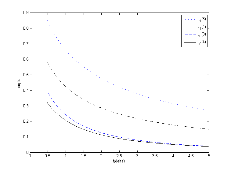
Figure 5: The payoffs of the middlemen are plotted as a function of $\delta$; note that $f(\delta)$ approaches $0$ as $\delta$ approaches $1$ and infinity as $\delta$ approaches $0$.

On the other hand, when $f(\delta)<0.49$, when using the “always-trade” strategy we will obtain a solution in which $z_{14}$ is negative. For example, when $f(\delta)=0.2$, $z_{14}=-0.1403$, which shows that the “always trade” strategy cannot be an equilibrium for this case. Recall here that $z_{14}=u_{1}(4)-u_{0}(4)-u_{1}(1)+u_{0}(1)$, which is the gain in trade when 1 sell an item to 4. If this value is negative, then 1 and 4 do not trade.

However, with $f(\delta)=0.2$, consider the strategy that avoids trade on the link $(1,4)$ and always trades otherwise. We will show that this is an equilibrium. To see this, first we observe that in this case the unique steady state of the Markov dynamic is $\mu_{3}=1/3$ and $\mu_{4}=1/2$. Similar to the previous case, we can set up a linear equation system for $z_{ij}$, where $(ij)\in\mathcal{E}=\{(1,3),(2,4),(3,5),(3,6),(4,6)\}$. Solving the system of linear equations, we get

$$z_{24}=0.5054,z_{13}=0.5755,z_{46}=0.8592,z_{36}=0.1344,z_{35}=0.9399.$$

Note that these values are all positive. Furthermore, the gain in trade between 1 and 4 is

$$u_{1}(4)-u_{0}(4)-u_{1}(1)+u_{0}(1)=f(\delta)\big{(}z_{46}-z_{24}-\frac{2}{3}z_{13}+0\big{)}=-0.0299\cdot f(\delta)<0.$$

This shows that, indeed, 1 and 4 do not have an incentive to trade. It is also clear here that, in this case, middlemen of type 3 have a higher payoff than middlemen of type 4.

Lastly, by considering all other pure strategies, we can conclude that for $f(\delta)=0.5$ the “always trade” strategy, and for $f(\delta)=0.2$ “avoiding trade on the link $(1,4)$ and always trades on all other links” are the unique pure equilibrium, respectively.

5 Comparative Studies With Patient Agents

In this section we will focus our comparative studies on the case when the discount factor $\delta$ approaches 1, which we sometimes refer to as when “agents are being patient” or the case of “vanishing bargaining friction.” In many cases, by considering this limiting case, we are either able to give a closed form characterization of the equilibrium, or present robust and general properties of any equilibrium.

We start by showing that as agents become patient, they will choose the cheapest trading routes (i.e. the routes with the smallest transaction costs) and intermediary fees per transaction will approach 0. We then give a closed form characterization for the equilibrium in a simple network containing two links. This shows how endogenous delay emerges even in this simple network. Finally, we use these two results to give an example of how changing the transaction costs in a network can have a fundamental and counter intuitive impact on agents’ payoffs.

5.1 Preference for Cheapest Trade Routes

THEOREM 5.1

Given a producer $p$, a consumer $c$, and any $\epsilon>0$, there exists $\delta^{*}$, such that for all $\delta>\delta^{*}$ and at any equilibrium the following is true. If $\lambda_{pm}>0$ and $\lambda_{mc}>0$ for a middlemen $m$, that is trade occurs along the route $p\rightarrow m\rightarrow c$, then the cost $C_{pm}+C_{mc}$ is the smallest among all trading routes between $p$ and $c$. Furthermore, the total surplus of producer $p$ and consumer $c$ satisfies $u_{1}(p)+u_{0}(c)\geq V_{v}-(C_{pm}+C_{mc})-\epsilon$.

Proof: Proof of Theorem 5.1: See Appendix 7.3.

Remark: The above result demonstrates a global-level efficiency that emerges in the equilibria of the local non-cooperative bargaining scheme if agents are patient enough: edges that are not along a cheapest path from any producer and consumer pair are never used, and middlemen who have no edges along a cheapest path from any producer and consumer pair see no trade.

Furthermore, $u_{1}(p)+u_{0}(c)\geq V_{v}-(C_{pm}+C_{mc})-\epsilon$ implies that the total surplus of producer $p$ and consumer $c$ is almost the entire trade surplus on the path $p\rightarrow m\rightarrow c$. This implies that as $\delta$ approaches 1, the intermediary’s fee that $j$ charges approaches 0. We discussed the intuition for this property in the introduction (Section 1). One important feature of our model that leads to this result is the fact that middlemen are long-lived and do not consume the good, while producers and consumer have limited supply and demand. Middlemen are eager to buy and sell quickly, while producers and consumers can wait because the discount rate $\delta$ is close to 1. It can be seen mathematically in the proof that when $\delta$ approaches 1, $z_{pm}$ and $z_{pc}$ approach 0. The term $z_{pm}+z_{mc}$ captures the gain of surplus for middlemen $m$ after buying an item from $p$ and selling it to $c$, assuming in both transactions, $m$ is the proposer.

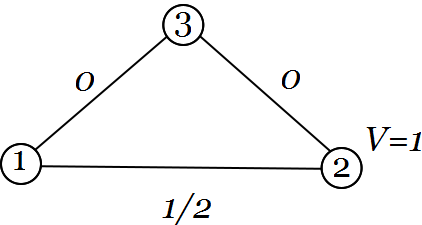
Figure 6: The trading network used to explore the choice of trade routes for $\delta\in(0,1)$.

Also notice that the selection of the cheapest routes does not hold when agents discount their payoff by $\delta$ much smaller than 1. To see this consider the network illustrated in Figure 6, where there are two paths connecting producer 1 and consumer 2. The direct link has a cost of 1/2, and both links connecting to middleman 3 costs 0. Hence, from Theorem 5.1, when $\delta$ is large enough trade will only occur through the middleman. However, when $\delta$ is small enough, even though the surplus of the direct trade is $1-1/2=1/2$, trade will happen on link $(1,2)$ when it is selected instead of waiting to trade through the middlemen of type $3$. In particular, assume the population at each node is the same, say $N$, and each link is selected uniformly at random so that $\pi_{ij}=1/3$ for all $(i,j)$.

Similar to the computation used in Theorem 4.1, let

$$\frac{1}{f(\delta)}:=\frac{\pi_{ij}}{2N\ln(1/\delta)}=\frac{1}{6N\ln(1/\delta)}.$$

It is then straightforward to check that the following is a limit stationary equilibrium.

• “Always trade” if $f(\delta)\geq 1/2$;

• Always trade on $(1,3)$, $(3,2)$ and avoid trade on $(1,2)$, if $f(\delta)<1/2$, which corresponds to $\delta\geq\exp\left(-\tfrac{1}{3N}\right)$.

In Figure 7, we plot the payoff of 1, 2, and 3 at this equilibrium as $f(\delta)$ varies from 0 to 2; these are decreasing as $f(\delta)$ increases.

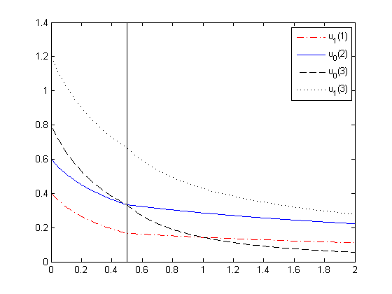
Figure 7: Agent payoffs as a function of $f(\delta)$.

5.2 Endogenous Delay

We now consider a simple network that consists of two links illustrated in Figure 8, which was again discussed in the introduction (Section 1). This network represents the simplest example where producers and consumers cannot trade directly. We fully characterize the limit stationary equilibrium in this example, which will be shown to be unique. Even in this simple network, we observe an interesting phenomenon of endogenous delay as part of the equilibrium. This is counterintuitive since in a full information dynamic bargaining model like ours, delay in trade does not enable agents to learn any new information, but only decreases the total surplus of trade. Therefore, the network structure and the combination of incentives of long-lived and short-lived agents are the main sources causing this inefficiency in bargaining.

Figure 8: A simple network to illustrate endogenous delay.

Assume $a$ and $b$ are transaction costs of the first and second link, also let $V$ be the value of the consumption of the good; without loss of generality, we will insist that trade is favorable so that $V>a+b$. The probabilities of using the links are then $\pi_{12}$ and $\pi_{23}$. We assume the population sizes at every node is equal, and without loss of generality, we assume $N_{1}=N_{2}=N_{3}=1$. We will show that in this simple network, the stationary equilibrium is unique, and we characterize the condition under which agents do not trade immediately.

THEOREM 5.2

In the limit of $\delta\rightarrow 1$, that is, when the agents are patient, there is always a unique limit stationary equilibrium. Furthermore, if $V\geq\left(1+\tfrac{\pi_{12}}{\pi_{12}+\pi_{23}}\right)a+b=:\bar{V}$, then trade always happens, otherwise there is a delay. The probability of trade on link $(1,2)$, $\lambda_{12}$, the probability of trade on link $(2,3)$, $\lambda_{23}$, and the equilibrium state and the payoffs of the middleman are given by

$$\lambda_{23} =1, \lambda_{12} =\begin{cases}1&\text{if }V\geq\bar{V}\\ \frac{\pi_{23}(V-b-a)}{\pi_{12}(2a+b-V)}&\text{otherwise}\end{cases},$$

$$\mu_{2} =\begin{cases}\frac{\pi_{12}}{\pi_{12}+\pi_{23}}&\text{if }V\geq\bar{V}\\ \frac{V-b-a}{a}&\text{otherwise}\end{cases},$$

$$u_{1}(2) =\begin{cases}\frac{(V-b)\left(2-\frac{\pi_{12}}{\pi_{12}+\pi_{23}}\right)-a}{1+\frac{\pi_{12}\pi_{23}}{(\pi_{12}+\pi_{23})^{2}}}&\text{if }V\geq\bar{V}\\ a&\text{otherwise}\end{cases}, u_{0}(2) =\begin{cases}\frac{V-\left(1+\frac{\pi_{12}}{\pi_{12}+\pi_{23}}\right)a-b}{1+\frac{\pi_{12}\pi_{23}}{(\pi_{12}+\pi_{23})^{2}}}&\text{if }V\geq\bar{V}\\ 0&\text{otherwise}\end{cases},$$

$$u_{0}(3) =\begin{cases}\frac{(V-b)\left(2-\frac{\pi_{12}}{\pi_{12}+\pi_{23}}\right)-a}{\frac{\pi_{12}+\pi_{23}}{\pi_{12}}+\frac{\pi_{23}}{\pi_{12}+\pi_{23}}}&\text{if }V\geq\bar{V}\\ 1-b-a&\text{otherwise}\end{cases}, u_{1}(1) =\begin{cases}\frac{V-\left(1+\frac{\pi_{12}}{\pi_{12}+\pi_{23}}\right)a-b}{\frac{\pi_{12}+\pi_{23}}{\pi_{12}}+\frac{\pi_{23}}{\pi_{12}+\pi_{23}}}&\text{if }V\geq\bar{V}\\ 0&\text{otherwise}.\end{cases}$$

Remark: As discussed in the introduction (Section 1), this can be compared with a model where each node consists of a single agent, where the sunk cost problem causes market failure, and no trade is the unique equilibrium. Here, however, we show that when the stock at the middlemen node is small, the search friction for a consumer to find a middlemen that owns an item increases the middlemen’s bargaining power, and this reestablishes trade with a positive probability.

From Theorem 5.2, we also see that trade always occurs on link $(2,3)$ but can be delayed at link $(1,2)$. Since the consumer is at the other end of link $(2,3)$, it stands to reason that there is no delay in the trade. However, at link $(1,2)$, any sale of the item results in a decreased likelihood of the trade at the same link (in the near future) owing to the search mechanism, and this opportunity cost introduces the delay in trade. Note also that with a delay in trade, the producer obtains no surplus! We will revisit this effect in the next section when we discuss the impact of the delay on the share of the surplus between the agents. Trade gets delayed when the value of the good is below a specific threshold. From the proof one can discern that the additional penalty term in the threshold is the product of the transaction cost at link $(1,2)$ and the stationary probability that the middleman possesses the good.

Proof: Proof of Theorem 5.2: See Appendix 7.4.

5.3 Share Of Surplus

Lastly, we consider the imbalance between the surplus of producers and consumers as a result of our decentralized trade model.

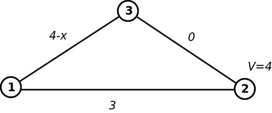
Figure 9: Triangle network with transaction costs.

Consider the following (also simple) network, where node 1 represents producers, node 2 represent consumers and node 3 represents middlemen, as illustrated in Figure 9. Again without loss of generality, we assume that$N_{1}=N_{2}=N_{3}=1$. We also assume that in our bargaining model, every link is selected uniformly at random, that is $\pi_{ij}=1/3$ for all $i\neq j$. Assume the consumer’s valuation for the good is $V_{2}=4$, and the transaction costs are the following: $C_{12}=3$, $C_{32}=0$ and $C_{13}=4-x$. We will investigate the equilibrium as $x$ changes. As $x$ increases, the transaction cost between $1$ and $3$ decreases, making the total trade surplus $\max\{4-3,4-(4-x)\}=\max\{1,x\}$ increase.

The surplus of producers in this example is understood as the payoff of agents at node 1 when owning an item: $u_{1}(1)$. On the other hand, the surplus of consumers in this example is the payoff of agents at node 2 when not owning an item: $u_{0}(2)$. According to the analysis in Section 5.1, as the discount rate $\delta$ approaches 1, trade will only goes through the cheapest route. Let $\bar{C}$ be the cost of this route, as seen in Section 5.1 we also have

$$\lim_{\delta\rightarrow 1}u_{1}(2)-u_{0}(2)-(u_{1}(1)-u_{0}(1))=\bar{C}.$$

This is equivalent to

$$\lim_{\delta\rightarrow 1}u_{0}(2)+u_{1}(1)=V_{2}-\bar{C}.$$

As shown in Section 5.1 this means that the total surplus of a producer and a consumer approaches the total trading surplus, and for every transaction, middlemen only make a vanishing amount of fee. As discussed in the introduction, this is because in our model, we assume producers and consumers are short-lived, while middlemen are long-lived and has to earn money by flipping the item. Thus, as $\delta$ approaches 1, while producers and consumers are patient, middlemen are eager to buy and sell quickly.

Now, in the example above, when considering the equilibrium payoff as $\delta$ approaches 1, we have if $x<1$ that producers and consumers will trade directly, and in this case producers and consumers equally share the surplus, giving them a surplus of $\tfrac{4-3}{2}=\tfrac{1}{2}$.

On the other hand, if $x>1$, then direct trade between producers and consumers is too expensive, and trade will go through middlemen at node 3. In the latter case, we will use the analysis in Section 5.2 to compute the equilibrium payoff, and we have

1. $1<x<4/3$: Seller’s surplus, $u_{1}(1)=0$ and consumer’s surplus $u_{0}(2)=x$, so that the consumers get all the trade surplus;

2. $4/3\leq x\leq 4$: Seller’s surplus, $u_{1}(1)=\frac{4-3/2(4-x)}{5/2}=\frac{3x-4}{5}$ and consumer’s surplus $u_{0}(2)=\frac{2x+4}{5}$.

This is illustrated in Figure 10.

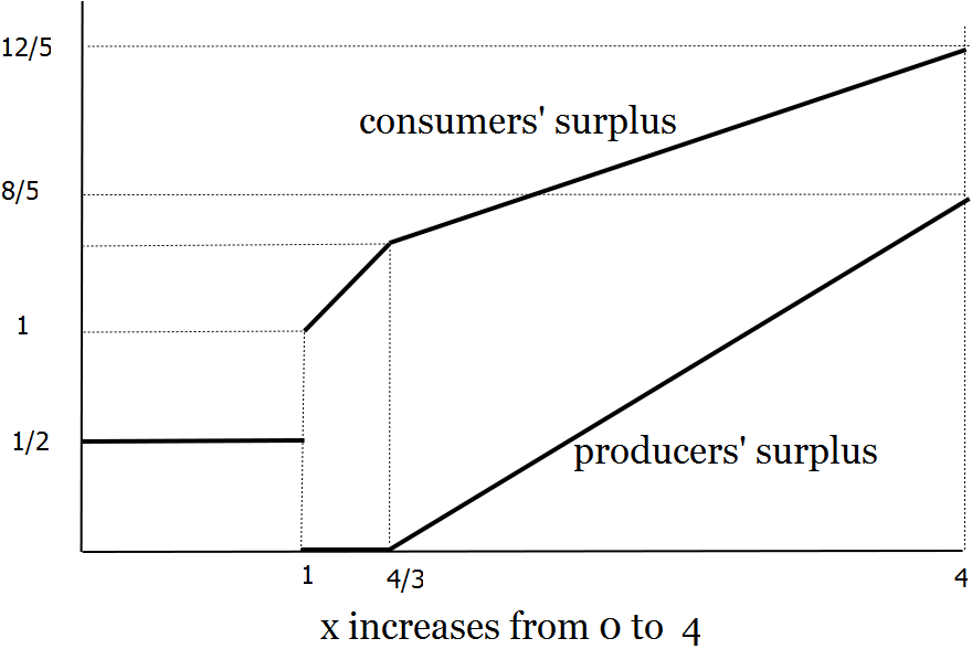
Figure 10: Surplus of producer and consumers as $x$ increases from 0 to 4

Even in this simple network, we observe quite an interesting phenomenon: there is a discontinuous shift in the trading pattern occurring in the network. If $x$ increases from $1$ to $4/3$, so that the transaction cost between 1 and 3, $C_{13}=4-x$, decreases, then the total surplus between producers and consumers increases, but producers are actually worse off because of this shift in the market structure. This also highlights how local adjustments by the producers could leave them in a worse-off position. Note that when $x=1$, at least two limit stationary exist: trade directly or via middlemen.

This example captures an interesting and counterintuitive phenomenon: as the transaction cost towards middlemen decreases, producers can be worse off, because the high cost of direct trading makes consumers refuse to trade directly and prefer to trade through middlemen. For example, in many supply chain networks, as these global networks get large, producers and consumers do not trade directly and several types of organizations emerge as middlemen. In many cases such as in coffee industry, producers (coffee farmers) obtain a very small fraction of surplus because there are too many middlemen in the supply chain network. See for example Bacon (2005) for a related empirical analysis of the coffee global supply chain and the recent shift in its market structure.

6 Conclusions And Future Work

In this paper we considered non-cooperative local bargaining over a trading network with a single type of good. In the limiting scenario of many agents, we showed the existence of a limit stationary equilibrium that can be characterized by a combination of the stationary probability of a trade happening on each link, the stationary distribution of the agents’ possessing the good, and the stationary payoffs of the agents. We then showed that when agents are patient enough, this limiting equilibrium can exhibit global efficiency. We applied this concept to several simple network structures to study the impact of the network on the bargaining power and surplus of all agents. In future work we plan to extend the results to more general networks, to include the analysis of losing or damaging the good and to rigorously connect the equilibria in the finite-player game to the limit stationary equilibria.

7 APPENDIX

7.1 Proof of Lemma 3.6

Since the transition matrix of the Markov process $\{\tilde{X}_{v}^{k}(t):v\in\mathcal{V}\}$ satisfies a Lipschitz condition, by an application of Kurtz’s Theorem (Ethier and Kurtz 2005, Th. 2.1, Chapter 11), we obtain a differential equation for the limiting process. The globally asymptotically stable state of the differential equation is a continuous function from the non-negative reals to $\prod_{p\in\mathcal{P}}[0,N_{p}]\times\prod_{m\in\mathcal{M}}[0,N_{m}]\times\prod_{c\in\mathcal{C}}[0,N_{c}]$. The limiting processes are given as follows for all $t\geq 0$,

$$\forall p\in\mathcal{P},\quad x_{p}(t)\equiv N_{p};\qquad\qquad\forall c\in\mathcal{C},\quad x_{c}(t)\equiv 0;$$

$$\forall m\in\mathcal{M},\quad\frac{dx_{m}(t)}{dt}=\left(1-\frac{x_{m}(t)}{N_{m}}\right)\sum_{p\in\mathcal{P}:(p,m)\in\mathcal{E}_{2}}\pi_{pm}\lambda_{pm}-\frac{x_{m}(t)}{N_{m}}\sum_{c\in\mathcal{C}:(m,c)\in\mathcal{E}_{3}}\pi_{mc}\lambda_{mc}$$ (18)

$$\qquad\qquad=\sum_{p\in\mathcal{P}:(p,m)\in\mathcal{E}_{2}}\pi_{pm}\lambda_{pm}-\frac{x_{m}(t)}{N_{m}}\left(\sum_{p\in\mathcal{P}:(p.m)\in\mathcal{E}_{2}}\pi_{pm}\lambda_{pm}+\sum_{c\in\mathcal{C}:(m,c)\in\mathcal{E}_{3}}\pi_{mc}\lambda_{mc}\right).$$ (19)

Using a quadratic Lyapunov function (square of the distance to the equilibrium point) it follows that there is a unique and globally asymptotically stable equilibrium point that is given by

$$\forall p\in\mathcal{P},\quad x_{p}^{*} =N_{p};\qquad\quad\forall c\in\mathcal{C},\quad x_{c}^{*}=0;$$

$$\forall m\in\mathcal{M},\quad x_{m}^{*} =N_{m}\frac{\sum_{p\in\mathcal{P}:(p,m)\in\mathcal{E}_{2}}\pi_{pm}\lambda_{pm}}{\sum_{p\in\mathcal{P}:(p,m)\in\mathcal{E}_{2}}\pi_{pm}\lambda_{pm}+\sum_{c\in\mathcal{C}:(m,c)\in\mathcal{E}_{3}}\pi_{mc}\lambda_{mc}}.$$

Therefore, the fraction of agents with the good satisfies

$$\forall p\in\mathcal{P},\quad\mu_{p} =1;\qquad\quad\forall c\in\mathcal{C},\quad\mu_{c}=0;$$

$$\forall m\in\mathcal{M},\quad\mu_{m} =\frac{\sum_{p\in\mathcal{P}:(p,m)\in\mathcal{E}_{2}}\pi_{pm}\lambda_{pm}}{\sum_{p\in\mathcal{P}:(p,m)\in\mathcal{E}_{2}}\pi_{pm}\lambda_{pm}+\sum_{c\in\mathcal{C}:(m,c)\in\mathcal{E}_{3}}\pi_{mc}\lambda_{mc}}.$$

Note that setting the right-hand side of (18) to zero, yields the balance condition (15).

For each $k$, it is easy to see that the Markov process is irreducible and has finite states, and so is positive recurrent. Thus, owing to the compact setting, the stationary measures of the scaled state processes converge to the point mass on the equilibrium point as $k$ increases without bound, see Benaim and Boudec (2011).

7.2 Proof of Theorem 3.5

We need to show that there exists $(\vec{\lambda},\vec{\mu},\vec{u},\vec{z})$ satisfying the following conditions:

1. Convergence: given the trading dynamics defined by $\vec{\lambda}$, the replicated economy converges to the steady state $\vec{\mu}$. According to Lemma 3.6, the convergence occurs and the dependence of $\vec{\mu}$ on $\vec{\lambda}$ is given by (16)-(17);

2. Payoff-state consistency: $\vec{u}$ and $\vec{z}$ need to satisfy equations (10)-(14); and

3. Payoff-dynamic consistency: if $z_{ij}>0$ then $\lambda_{ij}=1$; if $z_{ij}<0$ then $\lambda_{ij}=0$; and if $z_{ij}=0$, then $0\leq\lambda_{ij}\leq 1$.

Given $(\vec{\lambda},\vec{\mu},\vec{u})$, using equations (10)-(14) and (16)-(17) as well as the payoff-dynamic consistency above, we can obtain the following correspondence $(\vec{\Lambda},\vec{\mu}^{\prime},\vec{u}^{\prime})$, which we can write as follows,

$$F(\vec{\lambda},\vec{\mu},\vec{u})=(\vec{\Lambda},\vec{\mu}^{\prime},\vec{u}^{\prime}),$$

where

$$\forall p\in\mathcal{P}\quad\mu^{\prime}_{p} =1,$$

$$\forall c\in\mathcal{C}\quad\mu^{\prime}_{c} =0,$$

$$\forall m\in\mathcal{M}\quad\mu^{\prime}_{m} =\frac{\sum_{p\in\mathcal{P}:(p,m)\in\mathcal{E}_{2}}\pi_{pm}\lambda_{pm}}{\sum_{p\in\mathcal{P}:(p,m)\in\mathcal{E}_{2}}\pi_{pm}\lambda_{pm}+\sum_{c\in\mathcal{C}:(m,c)\in\mathcal{E}_{3}}\pi_{mc}\lambda_{mc}},$$

and for all $(i,j)\in\mathcal{E}$

$$\Lambda_{ij}= \{1\}\text{ if }u_{1}(j)-u_{0}(j)-(u_{1}(i)-u_{0}(i))-C_{ij}>0,$$

$$\Lambda_{ij}= \{0\}\text{ if }u_{1}(j)-u_{0}(j)-(u_{1}(i)-u_{0}(i))-C_{ij}<0,$$

$$\Lambda_{ij}= [0,1]\text{ if }u_{1}(j)-u_{0}(j)-(u_{1}(i)-u_{0}(i))-C_{ij}=0.$$

Furthermore,

$$\begin{split}\forall p\in\mathcal{P}\quad u^{\prime}_{0}(p)&=0,\\ \quad u^{\prime}_{1}(p)&=\sum_{c:(p,c)\in\mathcal{E}_{1}}\frac{\pi_{pc}}{2N_{p}\ln(1/\delta)}\max\{z_{pc},0\}+\sum_{m:(p,m)\in\mathcal{E}_{2}}\frac{\pi_{pm}}{2N_{p}\ln(1/\delta)}(1-\mu_{m})\max\{z_{pm},0\},\end{split}$$

$$\forall m\in\mathcal{M}\quad u^{\prime}_{0}(m) =\sum_{p:(p,m)\in\mathcal{E}_{2}}\frac{\pi_{pm}}{2N_{m}\ln(1/\delta)}\max\{z_{pm},0\},$$

$$\forall m\in\mathcal{M}\quad u^{\prime}_{1}(m) =\sum_{c:(m,c)\in\mathcal{E}_{3}}\frac{\pi_{mc}}{2N_{m}\ln(1/\delta)}\max\{z_{mc},0\},$$

$$\begin{split}\forall c\in\mathcal{C}\quad u^{\prime}_{0}(c)&=\sum_{p:(p,c)\in\mathcal{E}_{1}}\frac{\pi_{pc}}{2N_{c}\ln(1/\delta)}\max\{z_{pc},0\}+\sum_{m:(m,c)\in\mathcal{E}_{3}}\frac{\pi_{mc}}{2N_{c}\ln(1/\delta)}\mu_{m}\max\{z_{mc},0\},\\ \quad u^{\prime}_{1}(c)&=V_{c},\text{ where }\end{split}$$

$$z_{ij} =\Big{(}u_{1}(j)-u_{0}(j)-\Big{(}u_{1}(i)-u_{0}(i)\big{)}\Big{)}-C_{ij}\;\;\;\forall(i,j)\in\mathcal{E}_{1}\cup\mathcal{E}_{2}\cup\mathcal{E}_{3}.$$

It is straightforward to check that the function $F(\cdot,\cdot,\cdot)$ above satisfies all the requirements for Kakutani’s fixed-point theorem. The domain is a non-empty, compact and convex subset of a finite-dimensional Euclidean space. The mapping/correspondence has a closed-graph: since the mappings from $\vec{\lambda}$ to $\vec{\mu}^{\prime}$ and $\vec{\mu}$ to $\vec{u}^{\prime}$ are single-valued and continuous, we only need to satisfy this for the mapping from $\vec{u}$ to $\vec{\Lambda}$. For any sequence $(\vec{u}_{n},\vec{\Lambda}_{n})$ (in the domain) such $\lim_{n\rightarrow\infty}(\vec{u}_{n},\vec{\Lambda}_{n})=(\vec{u},\vec{\Lambda})$, it is easy to see that $\vec{\Lambda}$ must lie in the image of $\vec{u}$. Finally, the image of any point in the domain is non-empty, closed and convex. Therefore, there must be a fixed-point, and furthermore, by definition, any fixed point of this mapping is a limit stationary equilibrium.

7.3 Proof of Theorem 5.1

Consider equations (10), (11), (12) and (13). As $\delta$ approaches $1$, the $\log(1/\delta)$ term approaches $0$. Since $u_{1}(p)\in[0,\max_{c\in\mathcal{C}}V_{c}]$ for all $i\in\mathcal{P}$, and $u_{0}(c)\in[0,\max_{c\in\mathcal{C}}V_{c}]$ for all $c\in\mathcal{C}$, it has to be that given any $\epsilon>0$, there exists $\delta^{*}$ such that for all $\delta>\delta^{*}$, we have

$$z_{pc} \leq\epsilon\quad\forall(p,c)\in\mathcal{E}_{1},$$

$$z_{pm} \leq\epsilon\quad\forall(p,m)\in\mathcal{E}_{2},$$

$$z_{mc} \leq\epsilon\quad\forall(m,c)\in\mathcal{E}_{3}.$$

Now consider a pair of agents, one producer $p$ and consumer $c$. We have three cases then:

1. All trade routes from $p$ to $c$ have to visit some middleman. Let $m\in\mathcal{M}$ be one such middleman so that $(p,m)\in\mathcal{E}_{2}$ and $(m,c)\in\mathcal{E}_{3}$. The inequalities above then imply the following:

   $$u_{1}(m)-u_{0}(m) \geq u_{1}(c)-u_{0}(c)-C_{mc}-\epsilon,$$

   $$u_{1}(m)-u_{0}(m) \leq u_{1}(p)-u_{0}(p)+C_{pm}+\epsilon.$$

   These with $u_{0}(p)=0$ and $u_{1}(c)=V_{c}$ imply

   $$u_{1}(p)+u_{0}(c)\geq V_{c}-C_{pm}-C_{mc}-2\epsilon.$$

   Note that this inequality holds for every $m\in\mathcal{M}$ that lies along a trade route from $p$ to $c$. Therefore,

   $$u_{1}(p)+u_{0}(c)\geq V_{c}-\min_{\{m:(p,m)\in\mathcal{E}_{2}\text{ and }(m,c)\in\mathcal{E}_{3}\}}\Big{(}C_{pm}+C_{mc}\Big{)}-2\epsilon.$$

   Since $\epsilon$ can be chosen arbitrarily small, thus for any middleman $m$ who is not on a smallest transaction cost path from $p$ to $c$, we can choose $\delta$ close enough to 1 such that either $z_{pm}$ or $z_{mc}$ is strictly negative and so no trade can occur on the corresponding edge;

2. Notice that the same argument also works for the case, where if in addition to the middlemen, there also exists a direct link between $p$ and $c$. Then

   $$u_{1}(p)+u_{0}(c)\geq V_{c}-\min\bigg{(}C_{pc},\min_{\{m:(p,m)\in\mathcal{E}_{2}\text{ and }(m,c)\in\mathcal{E}_{3}\}}\Big{(}C_{pm}+C_{mc}\Big{)}\bigg{)}.$$

   Again it is clear that no trade occurs over links that are not part of a smallest transaction cost path from $p$ to $c$;

3. If $p$ and $c$ only have a direct route between them, then that is the only route via which trade can occur between this producer and consumer pair. Also, if no routes exist between $p$ and $c$, then obviously no trade occurs between these two agents.

7.4 Proof of Theorem 5.2

The equilibrium equations for this case are as follows:

$$u_{1}(1) =\frac{\pi_{12}}{2\ln(1/\delta)}(1-\mu_{2})\max\{z_{12},0\}, u_{0}(2) =\frac{\pi_{12}}{2\ln(1/\delta)}\max\{z_{12},0\},$$

$$u_{1}(2) =\frac{\pi_{23}}{2\ln(1/\delta)}\max\{z_{23},0\}, u_{0}(3) =\frac{\pi_{23}}{2\ln(1/\delta)}\mu_{2}\max\{z_{23},0\},$$

$$z_{12} =(u_{1}(2)-u_{0}(2)-u_{1}(1))-a, z_{23} =(V-u_{0}(3)-u_{1}(2)+u_{0}(2))-b,$$

$$\lambda_{12} \in\begin{cases}\{1\}&z_{12}>0\\ \{0\}&z_{12}<0\\ [0,1]&z_{12}=0\end{cases},\quad\lambda_{23}\in\begin{cases}\{1\}&z_{23}>0\\ \{0\}&z_{23}<0\\ [0,1]&z_{23}=0\end{cases}, \mu_{2} =\frac{\pi_{12}\lambda_{12}}{\pi_{12}\lambda_{12}+\pi_{23}\lambda_{23}}.$$

From the above is clear that $u_{1}(1)=(1-\mu_{2})u_{0}(2)$ and $u_{0}(3)=\mu_{2}u_{1}(2)$. Substituting these we get

$$z_{12}=\big{(}u_{1}(2)-(2-\mu_{2})u_{0}(2)\big{)}-a,\qquad z_{23}=\big{(}V-(1+\mu_{2})u_{1}(2)+u_{0}(2)\big{)}-b.$$

First consider the assumption that trade occurs with probability one on both links, i.e., $\lambda_{12}=\lambda_{23}=1$. This then implies that $\mu_{2}=\tfrac{\pi_{12}}{\pi_{12}+\pi_{23}}$, $z_{12},z_{23}\geq 0$ and we can substitute them directly into the equations for the payoffs. We then obtain the following linear equations in $u_{0}(2)$ and $u_{1}(2)$,

$$u_{0}(2)=\frac{u_{1}(2)-a}{\frac{2\ln(1/\delta)}{\pi_{12}}+(2-\mu_{2})},\quad u_{1}(2)=\frac{u_{0}(2)+V-b}{\frac{2\ln(1/\delta)}{\pi_{23}}+(1+\mu_{2})}.$$

We can take limits in the equations above as $\delta$ goes to $1$ (along an appropriate subsequence) to get

$$u_{0}(2)(2-\mu_{2})=u_{1}(2)-a,\qquad u_{1}(2)(1+\mu_{2})=u_{0}(2)+V-b.$$

Since the $\ln(1/\delta)$ terms vanish in the limit of $\delta$ going to $1$, so would the impact of the different population sizes. The unique solution of the above system of linear equations is

$$u_{1}(2)=\frac{(2-\mu_{2})(V-b)-a}{1+\mu_{2}-\mu_{2}^{2}},\quad u_{0}(2)=\frac{V-(1+\mu_{2})a-b}{1+\mu_{2}-\mu_{2}^{2}}.$$ (20)

It is easily seen that $u_{1}(2)\geq 0$ and $u_{0}(2)\geq 0$ if and only if $V\geq(1+\mu_{2})a-b=\bar{V}$, and at the equilibrium $z_{12}=z_{23}=0$.

For the remainder assume that $V<\bar{V}$. Consider the case that $\lambda_{23}=1$ and $0<\lambda_{12}<1$. This then implies that $z_{12}=0$, $z_{23}\geq 0$ and $\mu_{2}=\tfrac{\pi_{12}\lambda_{12}}{\pi_{12}\lambda_{12}+\pi_{23}}$. Again taking a limit of $\delta$ going to $1$ (along an appropriate subsequence), we also get $z_{23}=0$. If we solve (20), then the calculated $u_{0}(2)$ will be negative which then implies that at the equilibrium $u_{0}(2)=0$; note that $z_{12}=0$ for $\delta<1$ also yields the same conclusion. Now it follows that

$$u_{1}(2)=a,\;\mu_{2}=\frac{V-b-a}{a},\text{ and }\lambda_{12}=\frac{\pi_{23}(V-b-a)}{\pi_{12}(2a+b-V)}\in(0,1).$$

Since $V<\bar{V}=\left(1+\tfrac{\pi_{12}}{\pi_{12}+\pi_{23}}\right)a+b$, it also follows that $V<2a+b$ which ensures $\mu_{2}\leq 1$. Similarly, one can verify that $\lambda_{12}\in(0,1)$. Since the consistency conditions are met, we have an equilibrium.

The uniqueness of the solution in both cases also proves that the same solution holds along every subsequence of $\delta$ converging to $1$ (from below) so that the uniqueness of the equilibrium also follows. Finally, we can verify that there can be no other equilibria.

References

- Adlakha et al. (2010) Adlakha, Sachin, Ramesh Johari, Gabriel Y. Weintraub. 2010. Equilibria of dynamic games with many players: Existence, approximation, and market structure. http://arxiv.org/abs/1011.5537.
- Bacon (2005) Bacon, C. 2005. Confronting the coffee crisis: Can fair trade, organic, and specialty coffees reduce small-scale farmer vulnerability in northern Nicaragua? World Development (33).
- Benaim and Boudec (2011) Benaim, Michel, Jean-Yves Le Boudec. 2011. On mean field convergence and stationary regime. http://arxiv.org/abs/1111.5710. URL http://arxiv.org/abs/1111.5710.
- Biglaiser (1993) Biglaiser, Gary. 1993. Middlemen as experts. The RAND journal of Economics 212–223.
- Binmore and Herrero (1988) Binmore, Kenneth G, Maria J Herrero. 1988. Matching and bargaining in dynamic markets. The review of economic studies 55(1) 17–31.
- Blume et al. (2009) Blume, L.E., D. Easley, J. Kleinberg, E. Tardos. 2009. Trading networks with price-setting agents. Games and Economic Behavior 67(1) 36–50.
- Diamond (1982) Diamond, Peter A. 1982. Wage determination and efficiency in search equilibrium. The Review of Economic Studies 49(2) 217–227.
- Diamond and Maskin (1979) Diamond, Peter A, Eric Maskin. 1979. An equilibrium analysis of search and breach of contract, i: Steady states. The Bell Journal of Economics 282–316.
- Ethier and Kurtz (2005) Ethier, S. N., T. G. Kurtz. 2005. Markov processes: Characterization and convergence. 2nd ed. John Wiley & Sons.
- Gale (1987) Gale, Douglas. 1987. Limit theorems for markets with sequential bargaining. Journal of Economic Theory 43(1) 20–54.
- Gomes et al. (2010) Gomes, Diogo A., Joana Mohr, Rafael R. Souza. 2010. Mean field limit of a continuous time finite state game URL http://arxiv.org/abs/1011.2918.
- Graham and Méléard (1994) Graham, C., S. Méléard. 1994. Chaos hypothesis for a system interacting through shared resources. Probability Theory and Related Fields 100(2) 157–174.
- Guéant et al. (2011) Guéant, O., J.M. Lasry, P.L. Lions. 2011. Mean field games and applications. Paris-Princeton Lectures on Mathematical Finance 2010 205–266.
- Huang et al. (2010) Huang, Minyi, Peter E Caines, Roland P Malhamé. 2010. The nce (mean field) principle with locality dependent cost interactions. Automatic Control, IEEE Transactions on 55(12) 2799–2805.
- Lasry and Lions (2007) Lasry, J.M., P.L. Lions. 2007. Mean field games. Japanese Journal of Mathematics 2(1) 229–260.
- Lerner (1934) Lerner, A. P. 1934. The concept of monopoly and the measurement of monopoly power. The Review of Economic Studies 1(3) pp. 157–175.
- Li (1998) Li, Yiting. 1998. Middlemen and private information. Journal of Monetary Economics 42(1) 131–159.
- Manea (2011) Manea, Mihai. 2011. Bargaining in stationary networks. The American Economic Review 101(5) 2042–2080.
- Mortensen (1982) Mortensen, Dale T. 1982. The matching process as a noncooperative bargaining game. The economics of information and uncertainty. University of Chicago Press, 233–258.
- Nagurney et al. (2002) Nagurney, Anna, June Dong, Ding Zhang. 2002. A supply chain network equilibrium model. Transportation Research Part E: Logistics and Transportation Review 38(5) 281–303.
- Nguyen (2012) Nguyen, T. 2012. Local bargaining and endogenous fluctuations. Proc. 13th ACM Conf. on Electronic Commerce (EC-2012). Valencia, Spain.
- Rubinstein and Wolinsky (1987) Rubinstein, A., A. Wolinsky. 1987. Middlemen. The Quarterly Journal of Economics 102(3) 581–593.
- Rubinstein and Wolinsky (1985) Rubinstein, Ariel, Asher Wolinsky. 1985. Equilibrium in a market with sequential bargaining. Econometrica 53(5) 1133–50.
- Sznitman (1991) Sznitman, Alain-Sol. 1991. Topics in propagation of chaos. École d’Été de Probabilités de Saint-Flour XIX—1989, Lecture Notes in Math., vol. 1464. Springer, Berlin, 165–251. doi:10.1007/BFb0085169.
- Tirole (1988) Tirole, Jean. 1988. The theory of industrial organization. MIT Press.
- Wong and Wright (2011) Wong, Y.-Y., R. Wright. 2011. Buyers, sellers and middlemen: Variations on search-theoretic themes. Working Paper. Working Paper.
- Yavaş (1994) Yavaş, Abdullah. 1994. Middlemen in bilateral search markets. Journal of Labor Economics 406–429.