The Kitaev-Ising model,
Transition between topological and ferromagnetic order
Vahid Karimipour ,         Laleh Memarzadeh ,         Parisa Zarkeshian

Department of Physics, Sharif University of Technology,

P.O. Box 11155-9161, Tehran, Iran

We study the Kitaev-Ising model, where ferromagnetic Ising interactions are added to the Kitaev model on a lattice. This model has two phases which are characterized by topological and ferromagnetic order. Transitions between these two kinds of order are then studied on a quasi-one dimensional system, a ladder, and on a two dimensional periodic lattice, a torus. By exactly mapping the quasi-one dimensional case to an anisotropic XY chain we show that the transition occurs at zero $\lambda$ where $\lambda$ is the strength of the ferromagnetic coupling. In the two dimensional case the model is mapped to a 2D Ising model in transverse field, where it shows a transition at finite value of $\lambda$. A mean field treatment reveals the qualitative character of the transition and an approximate value for the transition point. Furthermore with perturbative calculation, we show that expectation value of Wilson loops behave as expected in the topological and ferromagnetic phases.

PACS: 03.67.-a, 03.65.Ud, 64.70.Tg, 05.50.+q

1 Introduction

In the study of many body systems, specially those inspired by quantum computation, a new paradigm is emerging, which embodies concepts such as topological order, topological phase, and topological phase transition. Contrary to the traditional Landau paradigm, topological phases are not characterized by local order parameters and topological phase transitions are not accompanied by spontaneous symmetry breaking. In addition to their interest in condensed matter physics[1], i.e. in fractional quantum Hall liquids [2] and quantum spin liquids [3], lattice models exhibiting topological order are of immense interest in the field of quantum computation and information [4], [5] due to their robustness against decoherence. The simplest such lattice models is the Kitaev model [4], although other models like color codes have also been introduced and extensively studied [6, 7]. The ground state of the Kitaev model on a surface of genus $g$, exhibits a $4g$-fold degeneracy which is directly related to the topology of the surface. Different ground states look exactly the same if probed by expectation values of local observable and are only distinguished if probed by global string-like operators going around non-trivial homology cycles of the surface. One can thus use these ground states to encode $2g$ qubits which are robust against errors and decoherence. Moreover one can do topological computations on these qubit states if one uses braiding and fusion of anyonic excitations of these models.

It is then natural to ask how much this topological order in the original Kitaev model or its generalizations to $Z_{N}$ group or the topological color codes [6, 7] are resilient against various kinds of perturbations [8, 9, 10, 11, 12, 13], temperature fluctuations [14] and so on. For example one can imagine that a strong magnetic field will eventually align all the spins in the direction of the magnetic field and the topological ordered phase transforms to a spin-polarized phase, [10, 15, 16] a phase which is easily recognized by local measurements of spins. Or one can imagine that at high enough temperature the topological phase transforms to a disordered phase [17], again recognizable locally. In these transitions a topologically degenerate ground space transforms to other forms of ground states. Phase transitions of this kind have been studied in [8, 9, 10, 11, 12, 13, 15, 16, 14, 18, 19, 20, 21].

It is the aim of this paper to study another kind of transition in these models. For concreteness we take the Kitaev model and ask how topological order can transform to ferromagnetic order. This transition is induced by Ising interaction and moreover it signifies a transition between two kinds of degenerate ground states. That is in the Kitaev limit the degeneracy comes from topology and in the Ising limit, it comes from symmetry. This will certainly add to our knowledge about topological order and the way it is either destroyed (i.e. by temperature or by magnetic fields) or changes to other types of local order (i.e. by ferromagnetic interactions).

To this end, we introduce a model in which Ising terms compete with Kitaev interactions, one to establish ferromagnetic order and the other to establish topological order. We study the model on both 2 dimensional torus and the quasi-one dimensional ladder network [22] which has almost all the characteristics of a topological model, i.e. topological degeneracy, robustness and anyonic excitations. Studying two different models has the benefit of understanding the role of dimension in this transition. To find the possibility of the transition and the transition point if any, we exactly map the problem of finding the ground state of the model to a simpler problem. In the ladder case, we map the model to a one-dimensional XY model, whose anisotropy is tuned by the ration of Ising to Kitaev couplings. This model is exactly solvable by free fermion techniques, its ground state is non-degenerate and smoothly varying, except at the extreme points (XX or YY interaction). Therefore in the case of ladder, there is no transition at finite Ising coupling. However in the 2D case, we exactly map the problem to the 2D Ising model in transverse field. The latter model has been studied using different methods [23, 24, 25] and is known to show a quantum phase transition. We show that the two sides of transition point correspond to topological and ferromagnetic order in the Kitaev-Ising model. This provides strong evidence for a transition between these two phases in the original model.

The structure of the paper is as follows: In section 2 we briefly review some preliminary facts on Kitaev model, emphasizing their difference on the torus and on the ladder. In section 3 we introduce the Kitaev-Ising model and solve it exactly on the ladder in subsection 4.1. In subsection 4.2, we map the Kitaev-Ising model to 2D Ising model in transverse field and analyze the degeneracy structure of the model and interpret it in terms of the original model. In an appendix, by a simple mean field analysis, we find the transition point which turns out to be near the actual one obtained by more accurate numerical means [26, 23, 24, 25]. To substantiate the idea of a phase transition between topological and non-topological phases, in section 5 we use the above mapping which facilitates an estimation of the expectation values of Wilson loops in the two regimes. These estimates indeed turns out to be as we expect, that is, the expectation value of a Wilson loop $\langle W_{C}\rangle$ behaves as the exponential of a quantity which is proportional to the perimeter of the $C$ near the Kitaev point and to the area enclosed by $C$ near the Ising point. The paper concludes with a discussion.

2 A brief account of the Kitaev Model

In this section we briefly review the Kitaev model [4] in order to set up the notation and use its main concepts in the sequel. Consider a lattice whose set of vertices, edges and plaquettes are respectively denoted by $V$, $E$ and $P$ respectively. The number of elements in these sets are respectively denoted by $|V|,|E|$ and $|P|$ respectively. Spin one-half particles live on the edges of this lattice and hence the dimension of the full Hilbert space is given by $2^{|E|}$. The Kitaev Hamiltonian on this lattice is given by

$$H_{Kitaev}:=-J\sum_{s\in V}A_{s}-K\sum_{p\in P}B_{p}$$ (1)

where

$$A_{s}:=\prod_{i\in s}\sigma_{i,x},\hskip 28.45274ptB_{p}:=\prod_{i\in\partial p}\sigma_{i,z}.$$ (2)

Here $i\in s$ means the edges incident on a vertex $s$ and $i\in\partial p$ means the edges on the boundary of a plaquette $p$. The coupling constants, $J,K$ and are taken to be positive. It is easily verified that all the vertex and plaquette operators commute with each other and square to the identity operator. The ground state is thus the common eigenvectors of all the vertex and plaquette operators with eigenvalue 1, that is $|\Phi\rangle$ is a ground state of the Kitaev model if it satisfies $A_{s}|\Phi\rangle=|\Phi\rangle,\ \ \ B_{p}|\Phi\rangle=|\Phi\rangle,\ \ \ \forall\ s,p.$

2.1 Kitaev Model on a two-dimensional periodic lattice (a torus)

For a 2D rectangular lattice of $N$ vertices, with periodic boundary conditions on both directions ( a torus), we have $|V|=N,|E|=2N,$ and $|P|=N$. Hence the dimension of the Hilbert space is $2^{2N}$ and we also have $N$ vertex operators $A_{s}$ and $N$ plaquette operators $B_{p}$ all commuting with each other and with the Hamiltonian. However there are two global constraints on the torus, namely

$$\prod_{s}A_{s}=I,\hskip 28.45274pt\prod_{p}B_{p}=I,$$ (3)

leading to ${2N-2}$ independent commuting operators and hence a 4-fold degeneracy of the ground state. In fact one notes that there are four string operators all commuting with the Hamiltonian, which are defined as follows:

$$T_{z}^{(1)}:=\prod_{i\in C_{1}}\sigma_{i,z},\hskip 28.45274ptT_{z}^{2}:=\prod_{i\in C_{2}}\sigma_{i,z},$$ (4)

$$T_{x}^{(1)}:=\prod_{i\in\tilde{C_{1}}}\sigma_{i,x},\hskip 28.45274ptT_{x}^{2}:=\prod_{i\in\tilde{C_{2}}}\sigma_{i,x},$$ (5)

where $C_{1}$ and $C_{2}$ are two homology cycles along the edges of lattice of the torus and $\tilde{C_{1}}$ and $\tilde{C_{2}}$ are two cycles running around the dual lattice (figure 1). Note that these operators, corresponding to homology cycles (curves which do not enclose any area) cannot be expressed in terms of vertex and plaquette operators. They have the following relations with each other:

$$T_{x}^{1}T_{z}^{1}=-T_{z}^{1}T_{x}^{1},\hskip 28.45274ptT_{x}^{2}T_{z}^{2}=-T_{z}^{2}T_{x}^{2}.$$ (6)

while all other relations are commutative ones. In other words, the operators $(T_{x}^{1},T_{z}^{1})$ and $(T_{x}^{2},T_{z}^{2})$ form two copies of the Pauli operators $\sigma_{x}$ and $\sigma_{z}$ which act to distinguish the four degenerate ground states of the Kitaev model and turn them into each other. That is, if we denote the four ground states by $|\Phi_{s_{1},s_{2}}\rangle,s_{1},s_{2}=0,1$, then we have

$$T_{z}^{1}|\Phi_{s_{1},s_{2}}\rangle=(-1)^{s_{1}}|\Phi_{s_{1},s_{2}}\rangle,\hskip 28.45274ptT_{z}^{2}|\Phi_{s_{1},s_{2}}\rangle=(-1)^{s_{2}}|\Phi_{s_{1},s_{2}}\rangle,$$ (7)

and

$$T_{x}^{1}|\Phi_{s_{1},s_{2}}\rangle=|\Phi_{s_{1}+1,s_{2}}\rangle,\hskip 28.45274ptT_{x}^{2}|\Phi_{s_{1},s_{2}}\rangle=|\Phi_{s_{1},s_{2}+1}\rangle.$$ (8)

Figure 1: (Color Online) The string operators $T_{z}^{1},T_{z}^{2}$ and $T_{x}^{1},T_{x}^{2}$. All of them commute with the pure Kitaev Hamiltonian ($H(\lambda=0)$). Only $T_{z}^{1}$ and $T_{z}^{2}$ commute with $H(\lambda)$ for all $\lambda$.

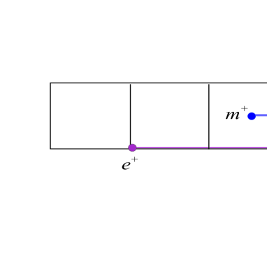
Figure 2: (Color Online) (a) The operators $T_{z}^{1}$ and $T_{x}^{1}$ on the ladder. $T_{z}^{1}$ is the product of $\sigma_{i,z}$ on the lower leg, while $T_{x}^{1}$ is the product of two $\sigma_{x}$’s one on each leg. Both commute with $H(\lambda=0)$, but only $T_{z}^{1}$ commutes with $H(\lambda)$. $T_{x}^{1}$ contains edges from the two legs. No operator containing only edges from one leg can substitute it. (b) Electric and magnetic anyons on the ladder.

2.2 The Kitaev Model on the quasi-one dimensional lattice (a ladder)

Since we will also study the Kitae-Ising Hamiltonian on the quasi-one dimensional systems, it is in order to note a few minor differences that the Kitaev model on the ladder has with the 2D case. Consider a ladder, as shown in figure (2), with $N$ plaquettes. There are $2N$ vertices and $3N$ edges. So the dimension of the Hilbert space is $2^{3N}$. We have periodic boundary condition only along the legs. The number of independent operators $B_{p}$ is equal to $N$, while the number of independent $A_{s}$ operators is $2N-1$, since $\prod_{s}A_{s}=I$. (There is no such constraint on the $B_{p}$ operators on the ladder). Therefore the total number of independent commuting operators is equal to $3N-1$ leading to a 2-fold degeneracy for the ground state. On the ladder only one pair of operators in (4, 5)) with their properties remain, which are denoted by $T_{z}^{1}$ and $T_{x}^{1}$ in figure (2). In fact the analogue of operator $T_{z}^{2}$ is an operator like $\sigma_{1,z}$ sitting on a single rung of the ladder, which no longer commutes with the Hamiltonian and the analog of operator $T_{x}^{2}$ is no longer independent from the vertex operators, since $T_{x}^{2}=\sigma_{1,x}\sigma_{2,x}\cdots\sigma_{N,x}=A_{1}A_{2}\cdots A_{N}$, where $A_{i}$ denote the vertex operators on the upper (or lower) leg of the ladder. This is in accord with the two-fold degeneracy of the ladder, that is if we denote the two ground states of the ladder by $|\Psi_{s}\rangle,\ s=0,1$, then we have

$$T_{z}^{1}|\Phi_{s}\rangle=(-1)^{s}|\Phi_{s}\rangle,\hskip 28.45274ptT_{x}^{1}|\Phi_{s}\rangle=|\Phi_{s+1}\rangle.$$ (9)

Note that the Kitaev model on a ladder, being a quasi-one dimensional system allows a restricted form of topological order. That is, concepts like area law for Wilson loops, or topological entanglement entropy may not apply to it. However there are still some topological characteristics in the ground states. First we have ground state degeneracy which does not come from symmetry. The two states being converted to each other by the global string operator $T^{1}_{x}$. Second we have a finite gap. Also the expectation value of any local operator, i.e one which does NOT traverse the the two legs of the ladder, is the same on the two ground states $|\Phi_{0}\rangle$ and $|\Phi_{1}\rangle$. In fact an operator which distinguishes the two ground states, should be one which commutes with the Hamiltonian and at the same time anti-commutes with $T^{1}_{z}$. Such an operator is given by $T_{x}^{1}$ which necessarily contains both legs of the ladder. (It is in this sense that no local operator (one defined on a single leg) can distinguishes the two ground states). Finally the system has anyonic exitations of electric and magnetic charges with integer charges and abelian statistics. In fact as shown in figure (2), an open string of $\sigma_{z}$ operators along the edges creates electric anyons at the end points, while an open string of $\sigma_{x}$ operators along the rungs creates magnetic anyons and cycling any electric anyon around a magnetic one creates a phase of (-1). Again the specific topology of the ladder reflects itself in the properties of its anyons in that, only electric anyons can move around the magnetic anyons.

Therefore many of the concepts pertaining to topological order are valid also for this quasi-one dimensional system. When we speak of topological order on the ladder, we mean this restricted meaning of the word. On 2D we do not have such a restriction.

3 The Kitaev-Ising model

We define the Kitaev-Ising Hamiltonian on any lattice as follows

$$H(\lambda):=H_{Kitaev}+\lambda H_{Ising},$$ (10)

in which $H_{Kitaev}$ is the usual Kitaev Hamiltonian (1) and $H_{Ising}$ is the Ising interaction between nearest neighbor links

$$H_{Ising}=-\sum_{\langle i,j\rangle}\sigma_{i,z}\sigma_{j,z},$$ (11)

where $\langle i,j\rangle$ means nearest-neighbor edges on the lattice. It is important to note that in the presence of the Ising interaction, the plaquette operators still commute with the full Hamiltonian, although the vertex operators no more do so:

$$[B_{p},H(\lambda)]=0,\ \ \ \forall p,\hskip 28.45274pt[A_{s},H(\lambda)]\neq 0.$$ (12)

Moreover from the four string operators, shown in figure (1), which commutes with the Kitaev Hamiltonian, only two retain this property in the presence of Ising interaction, namely

$$[T_{z}^{1},H(\lambda)]=0\hskip 28.45274pt[T_{z}^{2},H(\lambda)]=0,$$ (13)

but

$$[T_{x}^{1},H(\lambda)]\neq 0\hskip 28.45274pt[T_{x}^{2},H(\lambda)]\neq 0.$$ (14)

Correspondingly for the ladder, only the operator $T_{z}^{1}$ is defined which commutes with the Hamiltonian.

In view of the fact that $[B_{p},H(\lambda)]=0,\ \ \forall p,$ and $\lambda$ and the fact that in both limits (pure Kitaev and pure Ising) the ground states have eigenvalue $+1$ for all $B_{p}$’s, we conclude that the ground states of the Kitaev-Ising model lie in the subspace where $B_{p}=1$ for all the plaquettes. Denoting this subspace by ${\cal V}_{0}$,

$${\cal V}_{0}:=\{|\phi\rangle\ ,\ B_{p}|\phi\rangle=|\phi\rangle\}.$$ (15)

Therefore the restriction of the Hamiltonian to this subspace, $H_{0}(\lambda):=H(\lambda)\mid_{{\cal V}_{0}}$ is given by

$$H_{0}(\lambda)=-J\sum_{s}A_{s}-\lambda\sum_{\langle i,j\rangle}\sigma_{z,i}\sigma_{z,j}-K|P|,$$ (16)

where $|P|$ is the number of plaquettes in the lattice. Therefore the Ising coupling $\lambda$ or more precisely the ration $\frac{\lambda}{J}$ tunes the competition of ferromagnetic order and topological order. When this ration is zero we have pure Kitaev model and topological order, and when it is very strong, we have ferromagnetic order. In both cases we have degeneracy, but in one case the degeneracy is due to topology and in the other case it is due to symmetry. It is also interesting to note that the degeneracy of the ferromagnetic order is always two-fold, i.e. either all the spins are up or all are down, while the topological degeneracy is four-fold for the torus and two-fold for the ladder. In the subsequent sections we will understand how this order and the corresponding degeneracy changes as we change the parameter $\frac{\lambda}{J}$.

4 Solution of the Kitaev-Ising model

We showed that the ground states of the Kitaev-Ising model live in the subspace ${\cal V}_{0}$ defined in (15). The restriction of $H(\lambda)$ to this subspace is given by (16). To further diagonalize $H_{0}(\lambda)$, we construct a suitable basis for the subspace ${\cal V}_{0}$ and through this we transform $H_{0}(\lambda)$ to very simple models which have been studied previously. In fact, we will show that for the ladder, $H_{0}(\lambda)$ turns out to be the Hamiltonian of a one-dimensional XY chain, while for the 2D lattice, $H_{0}(\lambda)$ is the Hamiltonian of an Ising model in transverse field.

The way this basis is constructed is of utmost importance, in fact it should be constructed in such a way that all the operators in the Hamiltonian, i.e. the vertex and plaquette and also the Ising terms should be represented by nearest neighbor interactions between Pauli operators on virtual spins. Otherwise, one may come up with an inappropriate reduced Hamiltonian, one which may entail three or four-spin interactions or in case of two-body interactions it may entail longer than nearest-neighbor interactions. In other words, choosing this basis is a significant step in the process of diagonalization. Due to the difference between the topology of the ladder and the torus, we proceed in two different ways in construction of this basis. We start with the ladder and then study the case of 2D torus.

4.1 On the ladder

Consider the ladder shown in figure (3), where we take for definiteness the number of plaquettes to be an even number. We first note that the state

$$|\Phi_{0}\rangle:=\prod_{i=1}^{N}(1+B_{i})|+\rangle^{\otimes 3N},$$ (17)

where $|+\rangle$ is the positive eigenstate of $\sigma_{x}$, is a ground state of the pure Kitaev model, (one can easily check that it satisfies $A_{s}|\Phi\rangle=B_{p}|\Phi\rangle=|\phi\rangle$ for all $s$ and $p$). Consider the curve $C_{1}^{\prime}$ on the ladder (shown in figure (3)). This is a cycle going around the ladder and in fact it is equivalent to the straight curve $C_{1}$ shown in figure (2) (this equivalence is explained below). Therefore the other ground state of the pure Kitaev model on the ladder is nothing but

$$|\Phi_{1}\rangle:=\prod_{i\in C_{1}^{\prime}}\sigma_{i,z}|\Phi_{0}\rangle.$$ (18)

By equivalence of $C^{\prime}_{1}$ and $C_{1}$ we mean that the difference of $\prod_{i\in C^{\prime}_{1}}\sigma_{i,z}$ and $T_{z}^{1}:=\prod_{i\in C_{1}}\sigma_{i,z}$ is a product of $B_{i}$ operators which has no effect on $|\Phi_{0}\rangle$. In fact we can simply straighten a $\sqcap$ or a $\sqcup$ by multiplying with the $B$ inside them. We now construct the following set of un-normalized states

$$|\tilde{{\bf r}}\rangle:=|\tilde{r}_{1},\tilde{r}_{2},\tilde{r}_{3},\cdots\tilde{r}_{2N}\rangle=\prod_{i\in C^{\prime}_{1}}^{2{N}}\sigma_{i,z}^{r_{i}}|\Phi_{0}\rangle,\ \ \ \ r_{i}=0,1.$$ (19)

Clearly these states satisfy $B_{p}|\tilde{{\bf r}}\rangle=|\tilde{{\bf r}}\rangle$ for all $p$. We also note that

$$|\{\tilde{r}_{i}=0\}\rangle=|\Phi_{0}\rangle\ \ \ ,\ \ \ |\{\tilde{r}_{i}=1\}\rangle=|\Phi_{1}\rangle.$$

Moreover, they are orthogonal. For the proof of orthogonality, the basic idea to use, is that $|\Phi_{0}\rangle$ can be viewed simply as a linear combination of closed loops of spin $-$ particles in a background of all spin $+$ particles. Now if ${\bf r}\neq{\bf r^{\prime}}$, then it is easy to see that $\langle\tilde{{\bf r}}|\tilde{{\bf r}}^{\prime}\rangle\equiv\langle\Phi_{0}|\prod_{i\in C^{\prime}_{1}}\sigma_{i,z}^{r_{i}-r^{\prime}_{i}}|\Phi_{0}\rangle$ is the product of two states where one ($|\Phi_{0}\rangle$) has all closed loops and the other has open strings of spin down states, the product of which is zero. Finally their number is $2^{2N}$ which is equal to dimension of ${\cal V}_{0}$. Thus with proper normalization, they form an orthonormal basis for ${\cal V}_{0}$.

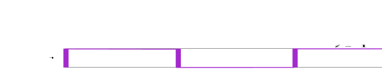
Figure 3: (Color Online) The curve used for generating an orthonormal basis in the sector ${\cal V}_{0}$ for the ladder network.

Why we have chosen this particular curve and this particular form for expressing the states of this sector? The answer lies in the nice form (i.e. nearest-neighbor two-body interaction) of the reduced Hamiltonian $H_{0}(\lambda)$. If we choose the curve as a simple straight form like $C_{1}$, then the states $|{\bf r}\rangle$ do not span the whole subspace ${\cal V}_{0}$.

To find $H_{0}(\lambda)$ in this new basis, we should determine the action of operators $A_{s}$ and also the Ising terms on these basis states. Due to the zigzag shape of the path and the appearance of the corresponding operators in the definition of $|\tilde{{\bf r}}\rangle$, we find that any vertex operator like $A_{i}$ in figure (3) when acting on the state (19) passes through all the operators except $\sigma_{z,i-1}$ and $\sigma_{z,i}$ with which it anticommutes. Thus the passage of $A_{i}$ through the whole chain of operators produces only the factor $(-1)^{r_{i-1}+r_{i}}$, hence the following effective operation on the basis states:

$$A_{i}|\tilde{{\bf r}}\rangle=Z_{i-1}Z_{i}|\tilde{{\bf r}}\rangle,$$ (20)

where $Z_{i}$ is the notation of Pauli operator $\sigma_{z}$ in this subspace.

Notation: Original Qubit states on the edges of the lattice are denoted without a $\tilde{}$. Thus $|0\rangle$ and $|1\rangle$ denote the computational basis states on the edges, $|0\rangle=|z,+\rangle$ and $|1\rangle=|z,-\rangle$. Pauli operators on these qubits are denoted by $\sigma_{x}$ and $\sigma_{z}$. The qubit states in (19) are always denoted by a $\tilde{}$ and the corresponding Pauli operators on these qubits are denoted by capital letters, $X$ and $Z$.

We now come to the Ising terms. Consider a group of Ising terms in one plaquette, the one shaded in figure (3). This can be written as

$$C_{i}:=\sigma_{i,z}\sigma_{i+1,z}+\sigma_{i,z}\sigma_{a,z}+\sigma_{i+1,z}\sigma_{i+2,z}+\sigma_{a,z}\sigma_{i+2,z}.$$ (21)

To express the action of $C_{i}$ in the basis (19), we note that this can be rewritten as

$$C_{i}:=\left(\sigma_{i,z}\sigma_{i+1,z}+\sigma_{i+1,z}\sigma_{i+2,z}\right)(1+B_{i}),$$ (22)

where $B_{i}$ is the operator corresponding to the same (shaded) plaquette. The operator $(1+B_{i})$ gives a factor of $2$ when acting on the state $|\tilde{{\bf r}}\rangle$ and the remaining $\sigma_{z,i}$ operators only flip the corresponding bit labels $\tilde{r}_{i}$. Hence the following effective action on the state:

$$C_{i}|\tilde{{\bf r}}\rangle=2\left(X_{i}X_{i+1}+X_{i+1}X_{i+2}\right)|\tilde{{\bf r}}\rangle,$$ (23)

where again $X_{i}$ is used to denote the first Pauli operator on the subspace ${\cal V}_{0}$. Putting everything together, we arrive at the following effective Hamiltonian on this subspace:

$$H_{0}(\lambda)=-J\sum_{i}Z_{i}Z_{i+1}-2\lambda\sum_{i}X_{i}X_{i+1}-K{N}.$$ (24)

This is an XY Hamiltonian in the absence of external magnetic field which has been studied extensively in the literature [27]. Its exact solution is provided by turning it into a free fermion model by Jordan-Wigner and Bogoluibov transformations. Its ground state is non-degenerate except at the extreme points $\lambda=0$ or $\lambda\longrightarrow\infty$. The ground state and the correlation functions show no non-analytical behaviour and no quantum phase transition occurs for finite $\lambda$. The only thing which happens is that the two-fold degeneracy breaks for any value of $\lambda$ except at the extreme points $\lambda=0,$ (Pure Kitaev) or $\lambda\longrightarrow\infty$ (Pure Ising). The end conclusion is that a transition from topological to ferromagnetic order does not occur for finite $\lambda$ in quasi-one dimensional systems.

Before leaving the subject of ladders, it is instructive to have a final look at the ground states of $H_{0}(\lambda)$ at the two extreme points. In these two limits, the ground state(s) of (24) should have simple product form (in terms of the labels $\tilde{r}_{i}$). Let us see if these are really what we expect for the Kitaev-Ising model. In the limit $\lambda=0$, equation (24) says that the virtual spins should all align either in the positive or negative $z$ direction, hence there are two degenerate ground states given by $|\tilde{\bf{0}}\rangle$ and $|\tilde{\bf{1}}\rangle$ respectively. As explained at the beginning of this subsection, these two states are clearly the two Kitaev states $|\Phi_{0}\rangle$ and $|\Phi_{1}\rangle$ on the ladder. The other limit, however, is more tricky to show. In the limit $\lambda\longrightarrow\infty$ all the virtual spins should align either in the positive $x$ or negative $x$ direction. We should show that this means that the actual spins on the edges of the ladder all align in the positive or negative $z$ direction. To see this consider the state $|\tilde{+},\tilde{+},\cdots\tilde{+}\rangle$. In view of the definition (19) and the structure of (17), and the fact that $|\tilde{+}\rangle\propto|\tilde{0}\rangle+|\tilde{1}\rangle$, this corresponds to

$$|\tilde{+},\tilde{+},\cdots\tilde{+}\rangle=\prod_{i\in C^{\prime}_{1}}(1+\sigma_{i,z})|\Phi_{0}\rangle=\prod_{i=1}^{N}(1+B_{i})|\Omega_{0}\rangle,$$ (25)

where $|\Omega_{0}\rangle:=\prod_{i\in C^{\prime}_{1}}(1+\sigma_{i,z})|+\rangle^{\otimes 3N}$ is a state on the ladder which we depict in figure (4). Here we have used the property $(1+\sigma_{z})|+\rangle=|0\rangle$. When the operators $1+B_{i}$ act on $|\Omega_{0}\rangle$, they turn the remaining $+$ states into $0$ and hence turn it into a ground state of the pure Ising model.

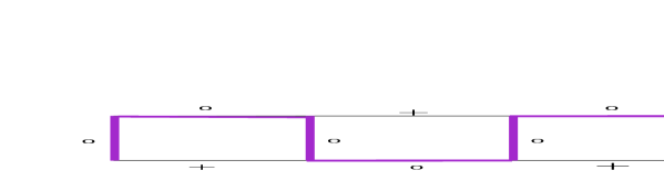
Figure 4: (Color Online) The state $\Omega_{0}$, defined in equation (25) and the following paragraph.

For the other state $|\tilde{-}\rangle$ a similar reasoning works in view of $(1-\sigma_{z})|+\rangle=|1\rangle$ where $|1\rangle$ is spin down in the z-direction.

4.2 On the two dimensional lattice

We now turn to the square lattice and show that $H_{0}(\lambda)$, describing the interactions of virtual spins, is in fact the Hamiltonian of a 2D Ising model in transverse magnetic field. This model is known to undergo a transition from ferromagnetic order to spin-polarized ordered phase. These phases, are shown to correspond respectively to topological and ferromagnetic ordered phases for the actual spins on the edges of the lattice.

To show this equivalence, we follow steps similar to the ones in previous section, however to represent the Hamiltonian in a simple form, we should choose an entirely different basis for the subspace ${\cal V}_{0}$.

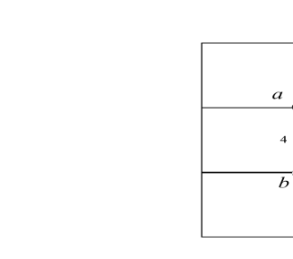
Figure 5: (Color Online) A portion of the lattice with their Kitaev and Ising interactions. The Ising interactions are between nearest-neighbor links. An Ising interaction like $\sigma_{3,z}\sigma_{4,z}$ (shown with the dash line) commutes with all the vertex and plaquette operators except with $A_{a}$ and $A_{a^{\prime}}$, to which it anti-commutes. Similarly an Ising term like $\sigma_{2,z}\sigma_{3,z}$ commutes with all but $A_{b}$ and $A_{b^{\prime}}$.

Let the lattice have $N$ plaquettes. Then the number of edges will be $2N$ and the number of vertices will be $N$. In a concise notation we have $|P|=N$, $|E|=2N$, and $|V|=N$. The dimension of the full Hilbert space is thus $2^{2N}$. ${\cal V}_{0}$ is the common eigenspace of all $B_{p}$ operators with eigenvalue $+1$. Since the number of independent plaquette operators is $N-1$, this means that $dim({\cal V}_{0})=\frac{2^{2N}}{2^{N-1}}=2^{N+1}$. Furthermore this subspace is decomposed to four different disconnected subspaces according to the eigenvalues of the global string operators $T_{z}^{1}$ and $T_{z}^{2}$. Let us denote this decomposition by

$${\cal V}_{0}={\cal V}_{0}^{++}\oplus{\cal V}_{0}^{+-}\oplus{\cal V}_{0}^{-+}\oplus{\cal V}_{0}^{--}.$$ (26)

Each subspace is $2^{N-1}$ dimensional. Consider now the states

$$|\tilde{{\bf r}}\rangle:=\prod_{i\in V}A_{i}^{r_{i}}|0\rangle^{\otimes|E|},\hskip 28.45274ptr_{i}=0,1.$$ (27)

Obviously these states satisfy $B_{p}|\tilde{{\bf r}}\rangle=|\tilde{{\bf r}}\rangle$. Moreover, when an $A_{i}$ acts on these states, it increases (by mod 2) the label $r_{i}$, hence the action of each $A_{i}$ on these states is represented by the bit-flip Palui operator $X_{i}$. In view of the constraint $\prod_{i\in E}A_{i}=1$, we have the equality $|\tilde{{\bf r}}\rangle=|\overline{\tilde{\bf r}}\rangle$, where $\overline{r_{i}}=r_{i}+1,\\ mod\ 2\ \forall i$. The subspace ${\cal V}_{0}^{++}$ is therefore span of the equivalence class of states $[|\tilde{{\bf r}}\rangle]=(|\tilde{{\bf r}}\rangle,|\overline{\tilde{{\bf r}}}\rangle)$. The other subspaces can be constructed similarly, i.e. ${\cal V}_{0}^{-+}=span\{[T_{x}^{1}|\tilde{{\bf r}}\rangle]=(T_{x}^{1}|\tilde{{\bf r}}\rangle,T_{x}^{1}|\overline{\tilde{{\bf r}}}\rangle)\}$.

When $\lambda\longrightarrow\infty$, (pure Ising model), the two ground states of the pure Ising model are clearly in the subspace ${\cal V}_{0}^{++}$, hence by the fact that $[T_{z}^{1},H(\lambda)]=[T_{z}^{2},H(\lambda)]=0$ and by continuity we find that the ground states of $H(\lambda)$ live in the subspace ${\cal V}_{0}^{++}$. Hereafter we will focus on this subspace.

To proceed we also assume that the lattice is bi-partite, i.e. $V=V_{A}\cup V_{B}$, where the vertices in $V_{A}$ are denoted by black circles in figure (5) and those of $V_{B}$ are denoted by white circles. Note that this puts a condition of even number of vertices in both directions. We need to find the action of the operators $A_{i}$ and the Ising terms on the states (27). It is obvious that the action of a vertex operator like $A_{i}$ on the state (27) is to simply flip the bit $r_{i}$, therefore $A_{i}$ acts on this subspace as $X_{i}$. Next we come to the Ising interactions. Consider the shaded plaquette in figure (5). The Ising interactions are given by

$$\sigma_{1,z}\sigma_{2,z}+\sigma_{2,z}\sigma_{3,z}+\sigma_{3,z}\sigma_{4,z}+\sigma_{4,z}\sigma_{1,z}=(\sigma_{1,z}\sigma_{2,z}+\sigma_{1,z}\sigma_{4,z})(1+B),$$ (28)

where $B$ is the plaquette operator containing the links 1, 2, 3, and 4. We now use the fact that an Ising interaction like $\sigma_{1,z}\sigma_{2,z}$ commutes with all the vertex operators and anit-commute with $A_{a}$ and $A_{a^{\prime}}$. This means that when $\sigma_{1,z}\sigma_{2,z}$ acts on the state $|\tilde{{\bf r}}\rangle$ it simply produces a factor $(-1)^{r_{a}+r_{a^{\prime}}}$, that is this operator acts on the subspace ${\cal V}_{0}^{++}$ as $Z_{a}Z_{a^{\prime}}$. Similarly the Ising term $\sigma_{1,z}\sigma_{4,z}$ commutes with all the vertex operators and anti-commutes with $A_{b}$ and $A_{b^{\prime}}$ and with the same reasoning the action of this operator on ${\cal V}_{0}^{++}$ is equivalent to $Z_{b}Z_{b^{\prime}}$. Therefore the Ising terms couple the nearest neighbor vertices of the sublattice $V_{A}$ and $V_{B}$ separately. Putting everything together we find the following effective Hamiltonian:

$$H=H_{A}+H_{B}-KN,$$ (29)

where $KN$ comes from the action of $\sum_{p}B_{p}$ on ${\cal V}_{0}$ and $H_{A}$ and $H_{B}$ are each a 2D Ising model in transverse field on sublattice $A$ and $B$ respectively:

$$H_{A}=-J\sum_{i\in A}X_{i}-2\lambda\sum_{\langle i,j\rangle\in A}Z_{i}Z_{j}$$ (30)

and

$$H_{B}=-J\sum_{i\in B}X_{i}-2\lambda\sum_{\langle i,j\rangle\in B}Z_{i}Z_{j}.$$ (31)

Here $\langle i,j\rangle$ means nearest-neighbor vertices on the corresponding sublattice. Note that the factor of $2$ in front of $\lambda$ comes from the factor $(1+B)$ in (28).

In this way the Kitaev-Ising Hamiltonian turns into the rather well-studied 2D Ising model in transverse field. The ferromagnetic order is controlled by the Ising coupling which tries to align all the virtual spins in the $+z$ or $-z$ direction. The transverse magnetic field controlled by $J$ competes with the Ising interaction and destroys the order if $J$ passes a critical value $J_{c}$. Density matrix renormalization group [24] gives a value of the critical magnetic field as $J_{c}\approx 6\lambda$. A simple mean field analysis (provided in the appendix) gives the value $J_{c}=8\lambda$. When $J>J_{c}$, the virtual spins try to align in the $+x$ direction. It is important to note that in the limit $J=0$ (or $\lambda\longrightarrow\infty$), the ground state of the virtual spin system is doubly degenerate, while in the limit $J\longrightarrow\infty$ (or $\lambda=0$) the ground state is unique and non-degenerate. What is interesting is that these two phases of virtual spins correspond to the topological and ferromagnetic phases of the actual spins on the edges of the lattice.

To see this correspondence, consider one of the Hamiltonians, say $H_{A}$. The $J$ term tends to align all the virtual spins in the $+x$ direction, while the $\lambda$ term tends to align them in the positive or negative $z$ direction. In the limit $\lambda\longrightarrow 0$ we have a unique ground state $|\tilde{+},\tilde{+},\cdots\tilde{+}\rangle$, while in the limit $\lambda\longrightarrow\infty$, there are two ground states $|\tilde{0},\tilde{0},\cdots\tilde{0}\rangle$ and $|\tilde{1},\tilde{1},\cdots\tilde{1}\rangle$. The same thing happens in sublattice $B$. Therefore in the limit $\lambda\longrightarrow 0$, there is a unique state, denoted by $(\tilde{+}_{A},\tilde{+}_{B})$, which is the topological ground state of the Kitaev state $|\Phi^{++}\rangle$, while in the limit $\lambda\longrightarrow\infty$, there are two ground states $(\tilde{0}_{A},\tilde{0}_{B})=(\tilde{1}_{A},\tilde{1}_{B})$ and $(\tilde{0}_{A},\tilde{1}_{B})=(\tilde{1}_{A},\tilde{0}_{B})$ which are the ferromagnetically ordered states, where all virtual spins are either up or down in the $z$ direction. Let us show this in a more explicit way. Consider the state denoted by $(\tilde{+}_{A},\tilde{+}_{B})$. In view of the notation (27), and the fact that $|\tilde{+}\rangle\propto|\tilde{0}\rangle+|\tilde{1}\rangle$ the state of actual spins corresponding to this state is given by $|\Phi^{++}\rangle:=\prod_{i\in V}(1+A_{i})|0\rangle^{\otimes E},$ which is a common eigenstate of all the $A_{i}$ and $B_{i}$ operators with eigenvalue $1$, hence a ground state of the pure Kitaev model.

In the other limit, the ground state $(\tilde{0}_{A},\tilde{0}_{B})$ denotes the state (27), where none of the $A_{i}$’s act on the state $|0\rangle^{\otimes|E|}$, hence this is nothing but a uniformly ordered ferromagnetic state in which all the spins are up in the $z$ direction, i.e. $|0\rangle^{\otimes|E|}$. We remind the reader that $(\tilde{0}_{A},\tilde{0}_{B})=(\tilde{1}_{A},\tilde{1}_{B})$, due to the constraint $\prod_{i\in V}A_{i}=1$. In other words, if we act on the state $|0\rangle^{\otimes|E|}$ by all the vertex operators $A_{i}$, nothing happens since the flipping actions of $A_{i}$ operators on the sublattice A are neutralized by those on sublattice B. To flip all the spins, one needs to apply the vertex operators $A_{i}$ on only one sublattice, hence the states $(\tilde{0}_{A},\tilde{1}_{B})=(\tilde{1}_{A},\tilde{0}_{B})$ correspond to the ferromagnetically ordered state $|1\rangle^{\otimes|E|}$.

5 Topological characteristics; estimates of Wilson loops

In order to justify the transition from topological to ferromagnetic order, we can estimate the value of a Wilsonian loop,

$$\langle W_{C}\rangle:=\langle\prod_{i\in C}\sigma_{i,x}\rangle,$$ (32)

where the expectation value is calculated in the ground state and $C$ is a closed curve on the dual lattice enclosing an area $S$, i.e. $C=\partial S$. Let us denote the perimeter of $\partial S$ by $|\partial S|$ and the area of ${S}$ by $|S|$. Then it is known that in the topological phase, the expectation value of this Wilson loop behaves as $e^{\beta|\partial S|}$, while in the non-topological phase it behaves as $e^{\gamma|S|}$, where $\beta$ and $\gamma$ are two constants [28]. The mapping of the Kitaev-Ising model to the 2D ITF model allows to obtain estimates of the Wilson loop in the two regimes perturbatively. To proceed we first note that in view of the definition of the vertex operators $A_{s}$ in (2), the operator $W_{C}$ can be written as

$$W_{C}=\prod_{s\in S}A_{s}\equiv\prod_{s\in S}X_{s},$$ (33)

where in the last equality we have used the equivalence of $A_{s}$ with $X_{s}$ on virtual spins (see the paragraph after Eq. 27), where the Hamitonian becomes a simple ITF Hamiltonian as in (30), we have to calculate the following expectation

$$\langle W_{C}\rangle=\frac{\langle\Psi|\prod_{s\in S}X_{s}|\Psi\rangle}{\langle\Psi|\Psi\rangle}.$$ (34)

where $|\Psi\rangle$ is the ground state of the 2D ITF model with the Hamiltonian given in (30). Note that in view of the decoupling between the two sublattices, we only consider one sublattice. Consider now the two limits, near-Kitaev and near-Ising separately.

5.1 Close to the Kitaev limit

In this limit, where $\gamma:=\frac{\lambda}{J}<<1$, we can take the Ising term in (30) as a perturbation to the magnetic field and approximate the ground state $|\Psi\rangle$ as a series

$$|\Psi\rangle=|\Psi_{0}\rangle+\gamma|\Psi_{2}\rangle+\gamma^{2}(|\Psi^{\prime}_{2}\rangle+|\Psi_{4}\rangle)+\cdots.$$ (35)

Here $|\Psi_{0}\rangle=|+\rangle^{\otimes N}$ is the ground state in the limit $\lambda=0$ and $|\Psi_{2}\rangle$ denotes the linear superposition of all states in which two adjacent spins have been flipped by the $Z_{i}Z_{j}$ terms. Note since we are doing an estimate and also we do not assume these states to be normalized, all numerical factors coming from perturbation expansion like energy differences and so on are absorbed in the definition of these states. Similarly, $|\Psi_{4}\rangle$ is the linear superposition of all states in which $4$ (two pairs of nearest-neighbor) spins have been flipped due to $(Z_{i}Z_{j})(Z_{k}Z_{l})$ terms and $|\Psi^{\prime}_{2}\rangle$ is the linear superposition of all states in which only two non-adjacent spins have been flipped by $(Z_{i}Z_{j})(Z_{j}Z_{k})$ term and so on. We then have

$$\langle\Psi|\Psi\rangle=\langle\Psi_{0}|\Psi_{0}\rangle+\gamma^{2}\langle\Psi_{2}|\Psi_{2}\rangle+O(\gamma^{3}).$$ (36)

We now note that $|\Psi_{2}\rangle$ can be broken up into three kinds of states, i.e.

$$|\Psi_{2}\rangle=|\Psi_{2}\rangle_{{}_{\overline{S}}}+|\Psi_{2}\rangle_{{}_{\underline{S}}}+|\Psi_{2}\rangle_{{}_{\partial S}},$$ (37)

where these states are described in figure (6). In view of this figure and the fact that $X_{i}|\pm\rangle=\pm|\pm\rangle$, we then have

$$W_{C}|\Psi_{2}\rangle=|\Psi_{2}\rangle_{{}_{\overline{S}}}+|\Psi_{2}\rangle_{{}_{\underline{S}}}-|\Psi_{2}\rangle_{{}_{\partial S}}.$$ (38)

Combining (37) and (38), and keeping all the terms up to order $\gamma^{2}$

$$\frac{\langle\Psi|W_{C}|\Psi\rangle}{\langle\Psi|\Psi\rangle}=1-2\gamma^{2}\ \ _{{}_{\partial S}}\langle\Psi_{2}|\Psi_{2}\rangle_{{}_{\partial S}}+O(\gamma^{3})$$ (39)

and since ${}_{{}_{\partial S}}\langle\Psi_{2}|\Psi_{2}\rangle_{{}_{\partial S}}=|\partial S|$, we find that close to the Kitaev limit, we have

$${\frac{\langle\Psi|W_{C}|\Psi\rangle}{\langle\Psi|\Psi\rangle}}\approx e^{-2\gamma^{2}|\partial S|}.$$ (40)

Therefore as expected close to the Kitaev limit, the expectation value of the Wilson loop behaves as the exponential of the perimeter of the loop, which is characteristic of the topological phase.

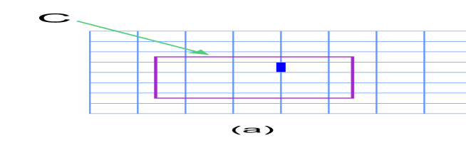
Figure 6: (Color Online) Different contributions to the state $|\Psi_{2}\rangle$. All the spins are in the state $|+\rangle$, except the two spins at the end of the bold link which have been flipped by the $ZZ$ interaction and are in the state $|-\rangle$. Figures (a), (b) and (c) exemplify contributions to the states $|\Psi_{2}\rangle_{\underline{S}}$, $|\Psi_{2}\rangle_{\overline{S}}$ and $|\Psi_{2}\rangle_{\partial{S}}$, respectively.

5.2 Close to the Ising limit

We now consider the Ising limit where $\frac{J}{\lambda}:=\frac{1}{\gamma}\leq 1$. Right at the Ising point, consider one of the degenerate ground states, say one in which all the spins are in the $+z$ direction, or using the quantum computation terminology, all the spins are in the state $0$. The magnetic field in (30) perturbs this uniform ground state by flipping spins one by one. These spins can be inside and or outside the loop $\partial S$. Denote the lattice points inside the loop by $S$ and the lattice points outside it by $\overline{S}$. Let us $|\phi_{k}\rangle|\chi_{k}\rangle$ denote the product state in which $|\phi_{k}\rangle$ is the state pertaining to $S$, and is the uniform superposition of all basis states in which exactly $k$ spins have been flipped to $|1\rangle$ (or $|-z\rangle$) and $|\chi_{k}\rangle$ is the state pertaining to $\overline{S}$ in which any number of spins have been flipped. Therefore the state $|\phi_{k}\rangle\chi_{k}\rangle$ is a state in which at least $k$ spins have been flipped. Then we can write the perturbative ground state as

$$|\Phi\rangle=\sum_{k=0}^{|S|}\gamma^{-k}|\phi_{k}\rangle|\chi_{k}\rangle.$$ (41)

Note that $|\chi_{k}\rangle$ is a state which is normalized to $O(1)$. The reason comes from perturbation theory, that is $|\chi_{k}\rangle$ is the superposition of states in $\overline{S}$ in which 0, 1, or more spins have been flipped. Note also that

$$\langle\phi_{k}|\phi_{k}\rangle=\left(\begin{array}[]{c}|S|\\ k\end{array}\right).$$

Since the operator $W_{C}=\prod_{i\in S}X_{i}$ flips all the spins inside $S$, we have

$$W_{C}|\Phi\rangle=\sum_{k=0}^{|S|}\gamma^{-k}|\phi_{|S|-k}\rangle|\chi_{k}\rangle.$$ (42)

Therefore we find

$$\langle\Phi|\Phi\rangle = \sum_{k=0}^{|S|}\gamma^{-2k}\ \langle\phi_{k}|\phi_{k}\rangle\ \langle\chi_{k}|\chi_{k}\rangle$$ (43)

$$\approx \sum_{k=0}^{|S|}\gamma^{-2k}\ \left(\begin{array}[]{c}|S|\\ k\end{array}\right)\approx(1+\gamma^{-2})^{|S|}.$$ (46)

On the other hand we find from (42) that

$$\langle\Phi|W_{C}|\Phi\rangle = \sum_{k=0}^{|S|}\gamma^{-|S|}\ \langle\phi_{k}|\phi_{k}\rangle\ \langle\chi_{k}|\chi_{k}\rangle$$ (47)

$$\approx \gamma^{-|S|}\sum_{k=0}^{|S|}\left(\begin{array}[]{c}|S|\\ k\end{array}\right)\approx\gamma^{-|S|}2^{|S|}.$$ (50)

Dividing (47) by (43) we find

$${\frac{\langle\Phi|W_{C}|\Phi\rangle}{\langle\Phi|\Phi\rangle}}\approx\left(\frac{2\gamma^{-1}}{1+\gamma^{-2}}\right)^{|S|}=e^{-|S|\ln\frac{1+\gamma^{2}}{2\gamma}}.$$ (51)

Therefore we have shown that close to the Kitaev and the Ising points, the Wilson loop behaves as expected, that is, its logarithm is proportional to the perimeter of the loop in the topological phase and proportional to the area in the ferromagnetic phase. All this has been made possible by mapping the system to the 2D Ising model in transverse field.

6 Discussion

We have introduced the Kitaev-Ising model, equation (10) as a model for studying the transition between topological order and ferromagnetic order in a lattice system. In particular we have shown that on the quasi-one dimensional system of the ladder (with periodic boundary condition), there is no quantum transition between these two kinds of order at finite $\lambda$, while in two dimensions a transition occurs at finite $\lambda$. This is reminiscent of what we have for thermal phase transitions based on symmetry breaking of discrete symmetries.

In the quasi-one dimensional case, we have exactly mapped the problem to the problem of finding the ground state of an XY chain in zero magnetic field for which exact solution by free fermion techniques is available. On a two dimensional lattice on the other hand, we have mapped the ground sector of the Kitaev-Ising Hamiltonian to two copies of Ising models in transverse magnetic fields, each defined on one sublattice, the latter model known to show sharp transition for finite $\lambda$. Although we have not attempted a numerical study of the model near the transition point, the equivalence with the 2D ITF model combined with the analysis of the degenerate structure of the ground states and their global properties in the two limits show that such a transition does occur for some finite $\lambda$. We have also estimated the Wilson loops and have shown that close to the Kitaev and Ising points, the logarithm of the expectation value of a Wilson loop is proportional to the perimeter of the loop in the topological phase and to the area enclosed by the loop in the ferromagnetic phase. It is also worth noticing an intriguing difference between the characteristic of the two different phases. In the topological phase, the four ground states are distinguished by loop operators $T^{1}_{z}$ and $T_{z}^{2}$ and are mapped to each other again by loop operators $T_{x}^{1}$ and $T_{x}^{2}$. In the ferromagnetic phase on the other hand, the two degenerate ground states are distinguished by a local operator $\sigma_{z}$, while the two ground states are mapped to each other by a global operator $\prod_{i\in E}\sigma_{i,x}$, encompassing the whole lattice. Therefore during the transition, the distinguishing loop operators shrink to points, while the transforming loop operators expand to the whole lattice.

This study can be extended in a few directions. First, one can use numerical techniques to determine the ground state and its properties as a function of the Ising coupling. Second it is desirable to generalize the analysis of this paper to the cases where the 2D lattice is not bipartite or the number of plaquttes in the ladder is not even (the simplifying assumptions made here) and to see if it leads to significantly different results.

7 Acknowledgements:

We would like to thank Saverio Pascazio, Razieh Mohseninia and Luigi Amico for interesting discussions during the early parts of this project. V. K. thanks Abdus Salam ICTP for its associateship award and support.

8 Appendix

In this appendix we briefly do a mean field analysis of the 2D Ising model in transverse field. Such an analysis reveals only a very qualitative feature of the transition. Using a product trial wave function $|\Psi\rangle=|\phi\rangle^{\otimes L}$ for the 2D ITF model (30), one needs to minimize the energy

$$\epsilon(|\phi\rangle):=-J\langle\phi|X|\phi\rangle-4\lambda\langle\phi|Z|\phi\rangle^{2}.$$

Taking $|\phi\rangle=\cos\frac{\theta}{2}|0\rangle+\sin\frac{\theta}{2}e^{i\phi}|1\rangle,$ leads to the following expression

$$\epsilon(\theta,\phi)=-J\sin\theta\cos\phi-4\lambda\cos^{2}\theta.$$ (52)

Minimizing this energy, one obtains that the nature of the mean field ground state changes at a critical value $\gamma_{c}=1$ ( $\gamma:=\frac{J}{8\lambda}$), that is the state which minimize the mean field energy is

$$|\phi\rangle=\left\{\begin{array}[]{ll}\frac{1}{\sqrt{2}}(|0\rangle+|1\rangle),&\hskip 28.45274pt\lambda<\frac{J}{8}\\ \cos\frac{\theta_{\gamma}}{2}|0\rangle\pm\sin\frac{\theta_{\gamma}}{2}|1\rangle&\hskip 28.45274pt\frac{J}{8}<\lambda\end{array}\right.$$ (53)

where

$$\sin\theta_{\gamma}=\frac{J}{8\lambda}.$$ (54)

From this mean field analysis we find the following expectation values $\langle X\rangle\equiv\langle A_{s}\rangle$ and $\langle Z\rangle\equiv\langle\sigma_{z}\rangle$, also shown in figure (7).

$$\langle X\rangle\equiv\langle A_{s}\rangle=\left\{\begin{array}[]{ll}1,&\hskip 28.45274pt\lambda<\frac{J}{8}\\ \frac{J}{8\lambda}&\hskip 28.45274pt\frac{J}{8}<\lambda\end{array}\right.$$ (55)

and

$$\langle Z\rangle\equiv\langle\sigma_{z}\rangle=\left\{\begin{array}[]{ll}0&\hskip 28.45274pt\lambda<\frac{J}{8}\\ \pm\sqrt{1-(\frac{J}{8\lambda})^{2}}&\hskip 28.45274pt\frac{J}{8}<\lambda.\end{array}\right.$$ (56)

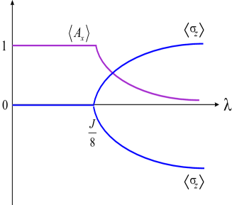
Figure 7: (Color Online) Mean field expectation values of $\langle X\rangle$ and $\langle Z\rangle$ on the 2D Ising model in transverse field, which are respectively equal to the $\langle A_{s}\rangle$ and $\langle\sigma_{z}\rangle$ on the original lattice. Note that after the transition point, the ground state becomes degenerate and the two ground states can be distinguished by a local order parameter $\langle\sigma_{z}\rangle$, hence two branches. The transition point predicted by mean-field is $\frac{J}{8}$, perturbation theory [26] and renormalization method [24] give a value $\approx\frac{J}{6}$.

References

- [1] X. -G. Wen, Quantum Field Theory of Many-body Systems (Oxford University Press, 2004).
- [2] X.-G. Wen and Q. Niu, Phys. Rev. B 41, 9377 (1990); Xiao-Gang Wen, Advances in Physics, 44, 405 (1995); H. L. Stormer, Rev. Mod. Phys. 71, S298S305 (1999).
- [3] S. V. Isakov, M. B. Hastings, and R. G. Melko, Nat. Phys. 7, 772 (2011); X. -G. Wen, Int. J. Mod. Phys. B 4, 239 (1990); S. Yan, D. A. Huse, and S. R. White, Science, 332, 1173 (2011).
- [4] A. Y. Kitaev, Ann. Phys. (N. Y.) 303, 2 (2003).
- [5] M. H. Freedman, A. Kitaev, and Z. Wang, Commun. Math. Phys. 227, 587 (2002); C. Nayak, S. H. Simon, A. Stern, M. Freedman, and S. Das Sarma, Rev.Mod. Phys. 80, 1083 (2008).
- [6] H. Bombin and M. A. Martin-Delgado, Phys. Rev. Lett. 97, 180501 (2006); Phys. Rev. B, 75:075103, 2007.
- [7] H. Bombin, and M. A. Martin-Delgado, New J. Phys. 13, 083006 (2011); H. Bombin, Ruben S. Andrist, Masayuki Ohzeki, Helmut G. Katzgraber, and M. A. Martin-Delgado, Phys. Rev. X 2, 021004 (2012).
- [8] S. Trebst, P. Werner, M. Troyer, K. Shtengel, and C. Nayak, Phys. Rev. Lett. 98, 070602 (2007); A. Hamma and D. A. Lidar, Phys. Rev. Lett. 100, 030502 (2008).
- [9] Alioscia Hamma, Lukasz Cincio, Siddhartha Santra, Paolo Zanardi, Luigi Amico, Local response of topological order to an external perturbation, arXiv:1211.4538
- [10] G bor B. Hal sz, Alioscia Hamma, Phys. Rev. A 86, 062330 (2012).
- [11] S.S. Jahromi, M. Kargarian, S Farhad Masoudi, and K.P. Schmidt, Topological color code in parallel magnetic field, arXiv:1211.1687.
- [12] M. D. Schulz, S. Dusuel, R. Orus, J. Vidal, and K. P. Schmidt, New Journal of Physics 14, 025005 (2012).
- [13] S. Dusuel, M. Kamfor, R. Orus, K. P. Schmidt, and J. Vidal, Robustness of a perturbed topological phase, Physical Review Letters, 106, 107203, (2011).
- [14] C. Castelnovo and C. Chamon, Phys. Rev. B 76, 184442 (2007); Phys. Rev. B 76, 174416 (2007).
- [15] J. Vidal, S. Dusuel, and K.P. Schmidt, Physical Review B 79, 033109 (2009).
- [16] J. Vidal, R. Thomale, K.P. Schmidt, and S. Dusuel, Physical Review B 80, 081104 (2009).
- [17] M. B. Hastings, Phys. Rev. Lett. 107, 210501 (2011); D. Mazac, A. Hamma, Ann. Phys. 327, 2096 (2012).
- [18] S. T. Flammia, A. Hamma, T. L. Hughes, and X.-G.Wen, Phys. Rev. Lett. 103, 261601 (2009).
- [19] A. Hamma, W. Zhang, S. Haas, and D. A. Lidar, Phys. Rev. B 77, 155111 (2008).
- [20] M. D. Schulz, S. Dusuel, K. P. Schmidt, J. Vidal, Topological Phase Transitions in the Golden String-Net Model, arXiv:1212.4109.
- [21] Wonmin Son, Luigi Amico, Rosario Fazio, Alioscia Hamma, Saverio Pascazio, and Vlatko Vedral, Europhys. Lett. vol. 95, 50001 (2011).
- [22] V. Karimipour, Phys. Rev. B 79, 214435 (2009).
- [23] A. Dutta, U. Divakaran, D. Sen, B. K. Chakrabarti, T. F. Rosenbaum and Gabriel Aeppli, Quantum phase transitions in transverse field spin models: From Statistical Physics to Quantum Information , arXiv:1012.0653v2.
- [24] M. S. L. du Croo de Jongh and J. M. J. van Leeuwen ,Phys. Rev. B 57, 8494 8500 (1998).
- [25] S. Dusuel, M. Kamfor, K. P. Schmidt, R. Thomale, J. Vidal, Phys. Rev. B 81, 064412 (2010).
- [26] P. Pfeuty and R. J. Elliott, J. Phys. C 4, 2370 (1971).
- [27] E. Lieb, T. Schultz, and D. Mattis, Ann. Physics 16, 407 (1961); E. Barouch and B. M. McCoy, Phys. Rev. A 2, 1075 (1970).
- [28] A. Hamma, W. Zhang, S. Haas, and D. A. Lidar, Phys. Rev. B 77, 155111 (2008).