Technical Report
Risk-neutral density recovery via spectral analysis

Abstract

In this paper, we propose a new method for estimating the conditional risk-neutral density (RND) directly from a cross-section of put option bid-ask quotes. More precisely, we propose to view the RND recovery problem as an inverse problem. We first show that it is possible to define restricted put and call operators that admit a singular value decomposition (SVD), which we compute explicitly. We subsequently show that this new framework allows us to devise a simple and fast quadratic programming method to recover the smoothest RND whose corresponding put prices lie inside the bid-ask quotes. This method is termed the spectral recovery method (SRM). Interestingly, the SVD of the restricted put and call operators sheds some new light on the RND recovery problem. The SRM improves on other RND recovery methods in the sense that 1) it is fast and simple to implement since it requires solution of a single quadratic program, while being fully nonparametric; 2) it takes the bid ask quotes as sole input and does not require any sort of calibration, smoothing or preprocessing of the data; 3) it is robust to the paucity of price quotes; 4) it returns the smoothest density giving rise to prices that lie inside the bid ask quotes. The estimated RND is therefore as well-behaved as can be; 5) it returns a closed form estimate of the RND on the interval $[0,B]$ of the positive real line, where $B$ is a positive constant that can be chosen arbitrarily. We thus obtain both the middle part of the RND together with its full left tail and part of its right tail. We confront this method to both real and simulated data and observe that it fares well in practice. The SRM is thus found to be a promising alternative to other RND recovery methods.

key words: Risk-neutral density; Nonparametric estimation; Singular value decomposition; Spectral analysis; Quadratic programming.

AMS subject classifications: 91G70, 91G80, 45Q05, 62G05

1 Introduction

1.1 The setting

Over the last four decades, the no-arbitrage assumption has proved to be a fruitful starting point that paved the way for the elaboration of a rich theoretical framework for derivatives pricing known today as arbitrage pricing theory. Among its numerous achievements, the arbitrage pricing theory has set forth two fundamental theorems. The First Fundamental Theorem of Asset Pricing (see [21, p.72]) proves that a market is arbitrage-free if and only if there exists a measure $\mathbb{Q}$ equivalent to the historical (or statistical) measure $\mathbb{P}$, which turns the underlying price process into a martingale. $\mathbb{Q}$ is therefore referred to as a martingale measure. The Second Fundamental Theorem of Asset Pricing (see [21, p.73]) proves in turn that this martingale measure is unique if and only if the market is complete (see [21, p.300] for terminology). Let us denote by $S_{\tau}$ the positive valued price of the underlying at a deterministic future date $\tau$ and by $\pi(S_{\tau})$ the payoff of a contingent claim maturing at time $\tau$. Let us moreover denote by $q$ the marginal density of $S_{\tau}$ under $\mathbb{Q}$ with respect to the Lebesgue measure on the positive real line, assuming that it exists. As initially proved in [10], the arbitrage price of this derivative security writes as its discounted expected payoff under $\mathbb{Q}$, that is,

$$e^{-r\tau}\mathbb{E}_{\mathbb{Q}}\pi(S_{\tau})=e^{-r\tau}\int_{x\geq 0}\pi(x)\mathbb{Q}(S_{\tau}\in dx)=e^{-r\tau}\int_{x\geq 0}\pi(x)q(x)dx,$$

where $r$ stands for the continuously compounded risk-free rate. It is a widely acknowledged fact that financial markets are incomplete, if only due to the presence of jumps in the underlying price process. In such a setting, and as described above, there exist possibly very many $q$s, and therefore, very many corresponding systems of arbitrage-free prices. Let us denote by $\mathscr{Q}$ the corresponding set of valid densities $q$. The elements $q$ of $\mathscr{Q}$ are most often referred to as risk-neutral densities (RNDs) and we will stick to this terminology in the sequel.

RNDs are of crucial interest for Central Banks and, in fact, most institutions and people concerned with financial markets since they represent the market sentiment about a given underlying price process at a future point in time (see [3]). They are also of crucial interest to the financial derivatives industry since the knowledge of $q$ allows to price new derivative securities in an arbitrage-free way with respect to traded ones. For these reasons, the literature related to risk-neutral density estimation is very extensive, the bulk of it dating back to the late 90’s and early 2k’s. It is not our purpose here to present an exhaustive review of this literature. Excellent and up-to-date reviews can in fact be found in [14, 17]. Older but still relevant ones can be found in [9, 3].

Among derivative securities, call and put options play a very particular role since they are actively traded in the market and thus believed to be efficiently priced. Let us recall that a call of strike $\xi$ and maturity $\tau$ gives its holder the right to buy the underlying security at maturity time $\tau$ at price $\xi$. It is an insurance against a rise in the price of the underlying. Its payoff writes $\pi(S_{\tau},\xi)=\theta(S_{\tau},\xi)=(S_{\tau}-\xi)^{+}$, where we have written $(x)^{+}=\max(x,0)$ for $x\in\mathbb{R}$. Conversely, a put option gives the right to sell the underlying security. It is an insurance against a fall in the underlying price and its payoff writes $\theta^{*}(S_{\tau},\xi)=(\xi-S_{\tau})^{+}$. Here and in what follows, we denote the strike price by $\xi$ and not by $k$, which will stand for a running index in $\mathbb{N}$.

According to the celebrated Breeden-Litzenberger formula, the second derivative of put and call prices with respect to their strike price both equal the discounted RND $e^{-r\tau}q$ (see [6]). Therefore, if a continuum of put or call prices were available in the market, we would have direct access to the RND by the latter formula. However, this is not the case and only a few strike prices around the forward price are quoted and actively traded at each maturity date. Depending on the market, we overall reckon from $5$ to $50$ quotes at a given maturity date $\tau$. To complicate the matter even more, quotes do not appear as a single price. Dealers quote in fact a bid price, at which they offer to buy the security, and an ask price, at which they offer to sell the security. The difference between both prices is referred to as the bid-ask spread. For an interesting insight into the nature of option quotes and sources of error in them, the reader is referred to, say, [16, p.786].

1.2 The problem and brief literature review

As detailed above, if traded puts and calls at a given maturity $\tau$ are arbitrage free, they must write as their expected discounted payoff with respect to a single RND $q$ drawn from the set $\mathscr{Q}$. Given the paucity of quoted option prices at a given maturity $\tau$ and the presence of a bid-ask spread, it is clear that many RNDs could in fact be hidden behind quoted option prices. Therefore, the RND quest is not that much about estimating the true RND that is used by the market for pricing purpose, since the nature of the quotes does not allow to identify it uniquely. It is rather more about recovering a valid RND, meaning an actual density function, to be chosen according to a criterion typically related to its smoothness or information content. Historically, three main routes have been used to recover a RND from quoted option prices: parametric methods, nonparametric methods and models of the underlying price process. Each of them have their pros and cons. Parametric methods are well adapted to small data sets and always recover a density. However, they constrain the RND to belong to a given parametric family. On the other hand, models of the underlying price process have been the first great success of arbitrage pricing theory with the celebrated geometric Brownian motion (see [4, 20]). However, the limitation of the log-normal distribution is now widely acknowledged and no satisfying stochastic process has yet been proposed that both reproduce accurately the dynamics of the underlying price process and be analytically tractable. Nonparametric methods circumvent both of these problems in the sense that they do not require any stringent assumption on the process generating the data (they are model-free) and can recover all possible densities. As a main drawback, these methods are often data intensive.

Let us briefly come back on some contributions to the nonparametric literature which are relevant to the present paper. We can classify nonparametric methods as follows.

• The expansion methods. It includes the Edgeworth (see [19]) and cumulant expansions (see [22]), which allow to estimate a finite number of RND cumulants. It also includes orthonormal basis methods such as Hermite polynomials (see [1]), which rely on well known Hilbert space techniques and give access to the middle part of the RND.

• The kernel regression methods. As a recent example, [2] have introduced a shape constrained local polynomial estimator of the RND. Notice that it performs estimation on the average quoted prices (that is, the average of the bid-ask quotes) and requires therefore to pre-process them in order to make them arbitrage-free. Moreover, the returned RND depends on the kernel chosen and it is not clear how it relates to the other valid RNDs in term of information content or smoothness.

• The maximum entropy method. It is introduced in [8, 23], where the RND $q$ is obtained via the maximization of an entropy criterion. According to [9, p.19], this method often gives bumpy (multimodals) estimates since it imposes no smoothness restriction on the estimated density. In addition, it is claimed in [18, p.1620], that this method presents convergence issues.

• Other methods, which do not belong to any of the three categories above. Among them, we can refer to the positive convolution approximation (PCA) of [5]. In practice, it fits a finite (but large) convex linear combination of normal densities to the average quoted put prices and approximates the RND by the weights of the linear combination. It thus presents similarities with [18], since it ultimately fits a discrete set of probabilities to the average quoted prices. We can also refer to the smoothed implied volatility smile method (SML) as in [14]. This method uses the Black-Scholes formula as a non-linear transform. It consists in fitting a polynomial through the implied volatilities obtained from average quoted prices, and using the continuum of option prices obtained in that way to get the RND via the Breeden-Litzenberger formula. [14] refines this method by taking the bid-ask quotes into account at the implied volatility fit stage. The SML method gives access to the middle part of the RND. [14] proposes in addition a method for appending generalized extreme value (GEV) tail distributions to it. The SML method is cumbersome and can seem a bit odd since it requires going from price space to implied volatility space, back and forth. It is claimed that it is outperformed in term of accuracy and stability by simpler parametric methods in [7].

1.3 Our results

In this paper, we propose to view the RND recovery problem as an inverse problem. We first show that it is possible to define restricted put and call operators that admit a singular value decomposition (SVD), which we compute explicitly. We subsequently show that this new framework allows to devise a simple and fast quadratic programming method to recover the smoothest RND that is consistent with market bid-ask quotes.

To be more precise, let us denote by ${\mathcal{I}}$ the segment $[0,B]$ of the positive real line. We define the restricted put and call operators, denoted by $\gamma^{*}$ and $\gamma$, from $\mathbb{L}_{2}{\mathcal{I}}$ into itself (see 2.1 and 2.2 below) and show that they are conjugates of one another. We prove that the resulting self-adjoint operator $\gamma^{*}\gamma$ is compact. As a consequence of the spectral theorem (see [15]), $\gamma^{*}$ admits a singular value decomposition with positive decreasing singular values. We prove that the corresponding singular bases are complete in $\mathbb{L}_{2}{\mathcal{I}}$ (see Theorem 3.1, item 3)) and compute them explicitly together with their singular values (see 1).

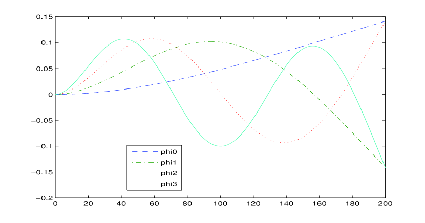
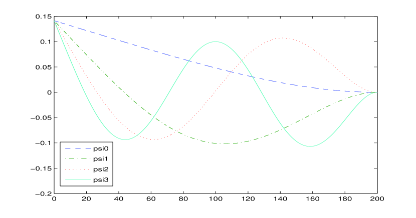
Figure 1: Here, we plot the first four elements of both singular bases. At the top we plot $\varphi_{k}$, $k=0,\ldots,3$. At the bottom, we plot $\psi_{k}$, $k=0,\ldots,3$.

To fix notations, we will write $(\varphi_{k})_{k\geq 0}$ and $(\psi_{k})_{k\geq 0}$ the two orthonormal families of $\mathbb{L}_{2}{\mathcal{I}}$ such that $\gamma^{*}\gamma\varphi_{k}=\lambda_{k}^{2}\varphi_{k}$, $\gamma\gamma^{*}\psi_{k}=\lambda_{k}^{2}\psi_{k}$, where $(\lambda_{k})_{k\geq 0}$ is a positive decreasing sequence of singular values. Precisely, we obtain explicitly,

$$\lambda_{k}=\left(\frac{B}{\rho_{k}}\right)^{2},$$

where

$$\rho_{k} =\frac{\pi}{2}+k\pi+(-1)^{k}\beta_{k}, k\in\mathbb{N},$$

and, for all $k\in\mathbb{N}$, $\beta_{k}$ is the smallest positive solution of the following fixed point equation in $u$,

$$\exp(\pi/2+k\pi+(-1)^{k}u)=\frac{1+\cos(u)}{\sin(u)}.$$

Interestingly, the positive sequence $(\beta_{k})$ decreases exponentially fast toward zero as detailed in Lemma 6.3. Therefore, the sequence of singular values $(\lambda_{k})_{k\geq 0}$ tends asymptotically toward zero at a rate of order $k^{-2}$. The RND recovery problem is therefore said to be mildly ill-posed with a degree of ill-posedness equal to $2$ (see [13, p.40]). Furthermore, for all $\xi\in{\mathcal{I}}$, we obtain,

$$\varphi_{k}(\xi) =\Bigl{(}a_{k,1}e^{\rho_{k}\xi/B}+a_{k,2}e^{-\rho_{k}\xi/B}\Bigr{)}+\Bigl{(}a_{k,3}\cos(\rho_{k}t/B)+a_{k,4}\sin(\rho_{k}\xi/B)\Bigr{)},$$

$$\psi_{k}(\xi) =\Bigl{(}a_{k,1}e^{\rho_{k}\xi/B}+a_{k,2}e^{-\rho_{k}\xi/B}\Bigr{)}-\Bigl{(}a_{k,3}\cos(\rho_{k}t/B)+a_{k,4}\sin(\rho_{k}\xi/B)\Bigr{)}.$$

where the coefficients $a_{k,i},i=1,\ldots,4$ are such that,

$$a_{k,1} =\frac{1}{\sqrt{B}}\frac{(-1)^{k}}{e^{\rho_{k}}+(-1)^{k}},$$

$$a_{k,2} =(-1)^{k}e^{\rho_{k}}a_{k,1}=\frac{1}{\sqrt{B}}\frac{1}{1+(-1)^{k}e^{-\rho_{k}}},$$

$$a_{k,3} =-\frac{1}{\sqrt{B}},$$

$$a_{k,4} =\frac{1}{\sqrt{B}}\frac{1-(-1)^{k}e^{-\rho_{k}}}{1+(-1)^{k}e^{-\rho_{k}}}.$$

Based on this new framework, we propose a spectral approach to RND recovery. It is fully nonparametric and can recover the restriction of any density to the interval ${\mathcal{I}}$. To that end, we notice that the singular bases functions $\varphi_{k}$ and $\psi_{k}$ are in fact oscillations $h_{k,2}$ at frequency $\rho_{k}/B$ carried by the exponential trend $h_{k,1}$ (see 6.2 and 6.1 for notations). Conveniently, smooth densities are therefore essentially captured by low singular spaces. The idea of recovering the smoothest density among the valid ones was initially suggested in [18]. Subsequently, [9] correctly pointed out that the smoothness criterion can be debated as it is difficult to give it an economic or even information theoretic meaning. Our spectral approach sheds some new light on this issue and makes it clear that the smoothness criterion is justified by the fact that the restricted call and put operators behave as low-pass frequency filters. It is therefore illusory to look for high frequency information about the RND in a set of quoted options prices, since this information has been drastically attenuated by the operator. The smoothness criterion arises therefore as a by-product of the spectral nature of the restricted put and call operators and might well not be an intrinsic property of the true RND. Interestingly, smooth densities are also easier to recover by nonparametric means.

In what follows, we exploit the rich framework offered by the SVD of the restricted put and call operators to recover the smoothest RND that is compatible with market quotes. As detailed in 7.1 below, the discounted restricted put operator coincides with the put price function (as a function of the strike) on ${\mathcal{I}}$. We therefore propose to recover the smoothest RND such that its image by the discounted restricted put operator $e^{-r\tau}\gamma^{*}$ lies in-between the bid-ask quotes (see 7.1). Conveniently, the singular bases present the property of being image of one another by second derivation modulo a multiplication by the corresponding singular value of $\gamma^{*}$ (see Theorem 6.1). This allows us to characterize the smoothness of the estimated RND directly in term of a quadratic form of the coefficients of the estimated put price function, which depends on the singular values of the restricted put operator (see Proposition 7.1). This crucial feature allows to recover the smoothest RND as the solution of a simple quadratic program, which takes the bid ask quotes as sole input. Our estimation method improves on existing ones in several ways, which we sum up here.

• It is fast and simple to implement since it only requires solution of a single quadratic program, while being fully nonparametric.

• It is robust to the paucity of price quotes since the smaller the number of quotes, the less constrained the quadratic program and thus the easier to solve.

• It takes the bid ask quotes as sole input and does not require any sort of smoothing or preprocessing of the data.

• It returns the smoothest density giving rise to price quotes that lie inside the bid ask quotes. The estimated RND is therefore as well-behaved as can be.

• It returns a closed form estimate of the RND on ${\mathcal{I}}$. We thus obtain both the middle part of the RND together with its left tail and part of its right tail. Interestingly, the left tail contains crucial information about market sentiments relative to a potential forthcoming market crash.

It is noteworthy that the singular vectors $\varphi_{0}$ and $\psi_{0}$ corresponding to the largest singular value $\lambda_{0}$ of $\gamma$ and $\gamma^{*}$ look themselves very much like cross sections of put and call prices, respectively (see 1). In that sense, they will be able to capture the bulk of the shape of a cross section of option prices, while the subsequent singular vectors will add corrections to this general behavior. This is a crucial feature of this SVD that leads us to think that the singular bases of the restricted pricing operators are appropriate tools to recover the RND $q$. Interestingly, the performance of our quadratic programming algorithm on real data is indeed quite convincing (see 8 for details).

Readers interested in appending a full right tail to this estimated RND are referred to [14], who proposes a simple method for smooth pasting of parametric GEV tail distributions to an estimated RND.

Here is the paper layout. We introduce the restricted call and put operators, $\gamma$ and $\gamma^{*}$, and operators derived therefrom in 2. We detail the properties of operators $\gamma^{*}\gamma$ and $\gamma\gamma^{*}$ on the one hand, and $\gamma$ and $\gamma^{*}$ on the other hand, in 3 and 4, respectively. Other results relative to these four operators are reported in 5. 6 gives explicit expressions for the $(\lambda_{k})$, $(\varphi_{k})$ and $(\psi_{k})$. The spectral recovery method (SRM) is detailed in 7. Finally, we run a simulation study in 8. An Appendix regroups some additional useful results.

2 Definitions and setting

Let us define the restricted call operator on the interval ${\mathcal{I}}=[0,B]$ as the operator $\gamma$ from $\mathbb{L}_{2}{\mathcal{I}}$ into $\mathbb{L}_{2}{\mathcal{I}}$ such that,

(2.1) $$(\gamma f)(\xi) =\int_{\mathcal{I}}\theta(\xi,x)f(x)dx, \xi\in{\mathcal{I}},f\in\mathbb{L}_{2}{\mathcal{I}},$$

$$\theta(\xi,x) =(x-\xi)^{+}.$$

It is a trivial fact that $\gamma f$ belongs indeed to $\mathbb{L}_{2}{\mathcal{I}}$. Let’s denote by $\langle.,.\rangle$ the usual scalar product on $\mathbb{L}_{2}{\mathcal{I}}$ and by $\|.\|_{\mathbb{L}_{2}{\mathcal{I}}}$ the associated norm. Now, it is enough to notice that for all $\xi,x\in{\mathcal{I}}$, $|\theta(\xi,x)|\leq B$ and apply Cauchy-Schwartz inequality to obtain,

$$\|\gamma f\|_{\mathbb{L}_{2}{\mathcal{I}}}^{2}\leq\int_{\mathcal{I}}d\xi\left(\int_{\mathcal{I}}dx|\theta(\xi,x)||f(x)|\right)^{2}\leq B^{4}\|f\|_{\mathbb{L}_{2}{\mathcal{I}}}^{2}<\infty.$$

The adjoint operator $\gamma^{*}$ of $\gamma$ is such that, for all $f,g\in\mathbb{L}_{2}{\mathcal{I}}$,

$$\langle\gamma^{*}f,g\rangle =\langle f,\gamma g\rangle$$

$$=\int_{\mathcal{I}}duf(u)\int_{\mathcal{I}}dx\theta(u,x)g(x)$$

$$=\int_{\mathcal{I}}dxg(x)\int_{\mathcal{I}}du\theta(u,x)f(u).$$

Hence

(2.2) $$\gamma^{*}f(\xi) =\int_{\mathcal{I}}\theta^{*}(\xi,x)f(x)dx, \xi\in{\mathcal{I}},f\in\mathbb{L}_{2}{\mathcal{I}},$$

$$\theta^{*}(\xi,x) =\theta(x,\xi).$$

So that $\gamma^{*}$ is nothing but the restricted put operator on the interval ${\mathcal{I}}$. In particular, we can write

(2.3) $$\gamma^{*}\gamma f(\xi) =\int_{\mathcal{I}}\vartheta_{1}(\xi,x)f(x)dx, \xi\in{\mathcal{I}},f\in\mathbb{L}_{2}{\mathcal{I}},$$

(2.4) $$\gamma\gamma^{*}f(\xi) =\int_{\mathcal{I}}\vartheta_{2}(\xi,x)f(x)dx, \xi\in{\mathcal{I}},f\in\mathbb{L}_{2}{\mathcal{I}},$$

where

$$\vartheta_{1}(\xi,x) =\int_{\mathcal{I}}du\theta^{*}(\xi,u)\theta(u,x)$$

$$=\int_{\mathcal{I}}du(\xi-u)^{+}(x-u)^{+}=\int_{0}^{\xi\wedge x}du(\xi-u)(x-u)$$

$$=\xi x(\xi\wedge x)-(\xi+x)(\xi\wedge x)^{2}/2+(\xi\wedge x)^{3}/3,$$

and

$$\vartheta_{2}(\xi,x) =\int_{\mathcal{I}}du\theta(\xi,u)\theta^{*}(u,x)$$

$$=\int_{\mathcal{I}}du(u-\xi)^{+}(u-x)^{+}=\int_{\xi\vee x}^{B}du(u-\xi)(u-x)$$

$$=\xi x(B-\xi\vee x)-(\xi+x)(B-\xi\vee x)^{2}/2+(B-\xi\vee x)^{3}/3.$$

Let us now turn to the detailed inspection of these operators.

3 Results relative to $\gamma^{*}\gamma$ and $\gamma\gamma^{*}$

Let us denote by $\mathcal{R}(\kappa)$ the range of an operator $\kappa$ of $\mathbb{L}_{2}{\mathcal{I}}$ and by $\mathcal{N}(\kappa)$ its null space (see [12, p.23]). Obviously both $\gamma^{*}\gamma$ and $\gamma\gamma^{*}$ are self-adjoint. This translates into the fact that their kernels are symmetric (meaning $\vartheta_{i}(\xi,x)=\vartheta_{i}(x,\xi)$). In addition, both $\vartheta_{1}$ and $\vartheta_{2}$ are continuous on the bounded square ${\mathcal{I}}\times{\mathcal{I}}$. Therefore, the associated operators are compact (see [12, Ex. 4.8.4, p.172]). As such, they verify the spectral theorem (see [12, Th. 4.10.1, 4.10.2, p.187-189]).

Theorem 3.1.

Given the operators $\gamma^{*}\gamma$ and $\gamma\gamma^{*}$ defined in 2.3 and 2.4 above, we have the following results.

1. The operators $\gamma^{*}\gamma$ and $\gamma\gamma^{*}$ are compact and self-adjoint. As such, they admit countable families of orthonormal eigenvectors $(\varphi_{k})$ and $(\psi_{k})$ associated to the same positive decreasing sequence of eigenvalues $\lambda^{2}_{k}$, which are complete in $\mathcal{R}(\gamma^{*}\gamma)$ and $\mathcal{R}(\gamma\gamma^{*})$, respectively.

2. Besides, we have

   $$\mathcal{R}(\gamma^{*}\gamma) \subset\mathbb{L}_{2}{\mathcal{I}}\cap\mathcal{C}^{4}{\mathcal{I}},$$

   $$\mathcal{R}(\gamma^{*}\gamma) \subset\mathbb{L}_{2}{\mathcal{I}}\cap\mathcal{C}^{4}{\mathcal{I}},$$

   where $\mathcal{C}^{4}{\mathcal{I}}$ stands for the set of four times differentiable functions on ${\mathcal{I}}$.

3. Furthermore, the orthonormal families $(\varphi_{k})$ and $(\psi_{k})$ are complete in $\mathbb{L}_{2}{\mathcal{I}}$. In other words, they are both orthonormal bases of $\mathbb{L}_{2}{\mathcal{I}}$. In fact, we can write

   $$\mathbb{L}_{2}{\mathcal{I}} =\overline{\mathcal{R}(\gamma^{*}\gamma)}=\text{Span}\{\varphi_{k},k\in\mathbb{N}\},$$

   $$=\overline{\mathcal{R}(\gamma\gamma^{*})}=\text{Span}\{\psi_{k},k\in\mathbb{N}\},$$

   where $\overline{\mathcal{R}(\gamma^{*}\gamma)}$ stands for the closure of $\mathcal{R}(\gamma^{*}\gamma)$ in $\mathbb{L}_{2}{\mathcal{I}}$ (see [12, p.16]) and $\text{Span}\{\varphi_{k},k\in\mathbb{N}\}$ for the set of (potentially infinite) linear combinations of elements $\varphi_{k}$.

4. Therefore, $\gamma^{*}\gamma$ and $\gamma\gamma^{*}$ are both invertible and admit the fourth order differential operator $\partial_{\xi}^{4}$ as an inverse (see [12, p.155] for terminology). More precisely, we have got

   $$\partial_{\xi}^{4}\gamma^{*}\gamma f =f, \forall f\in\mathbb{L}_{2}{\mathcal{I}},$$

   $$\gamma^{*}\gamma\partial_{\xi}^{4}f =f, \forall f\in\mathcal{R}(\gamma^{*}\gamma),$$

   and idem for $\gamma\gamma^{*}$.

5. Finally, we have the following spectral decompositions,

   $$f =\sum_{k\geq 0}\langle f,\varphi_{k}\rangle\varphi_{k}, f \in\mathbb{L}_{2}{\mathcal{I}},$$

   $$\gamma^{*}\gamma f =\sum_{k\geq 0}\lambda_{k}^{2}\langle f,\varphi_{k}\rangle\varphi_{k}, f \in\mathbb{L}_{2}{\mathcal{I}},$$

   and

   $$f =\sum_{k\geq 0}\langle f,\psi_{k}\rangle\psi_{k}, f \in\mathbb{L}_{2}{\mathcal{I}},$$

   $$\gamma\gamma^{*}f =\sum_{k\geq 0}\lambda_{k}^{2}\langle f,\psi_{k}\rangle\psi_{k}, f \in\mathbb{L}_{2}{\mathcal{I}}.$$

Proof.

As detailed above, 1) follows directly from the spectral theorem. 2) follows directly from the kernel representations in 2.3 and 2.4. It can also be seen from the fact that, for any $f\in\mathbb{L}_{2}{\mathcal{I}}$, both $\gamma f$ and $\gamma^{*}f$ are twice differentiable, which follows by simple inspection of 2.1 and 2.2. 3) follows directly from Proposition 5.1 below. 4) is a direct consequence of Lemma 8.1 below. Finally, 5) follows directly from 1) and 3). ∎

4 Results relative to $\gamma$ and $\gamma^{*}$

The following theorem details the properties of the restricted put and call operators. It builds upon Theorem 3.1 above.

Theorem 4.1.

Given operators $\gamma$ and $\gamma^{*}$ defined in 2.1 and 2.2 above, we have the following results.

1. Consider the sequence of positive decreasing singular values $\lambda_{k}$ and singular vectors $(\varphi_{k})$ and $(\psi_{k})$ defined in Theorem 3.1 above. The restricted put and call operators $\gamma^{*}$ and $\gamma$ are such that, for all $k\geq 0$,

   $$\gamma\varphi_{k} =\lambda_{k}\psi_{k}, \gamma^{*}\psi_{k} =\lambda_{k}\varphi_{k}.$$

2. Besides, we have

   $$\mathcal{R}(\gamma^{*}) \subset\mathbb{L}_{2}{\mathcal{I}}\cap\mathcal{C}^{2}{\mathcal{I}},$$

   $$\mathcal{R}(\gamma) \subset\mathbb{L}_{2}{\mathcal{I}}\cap\mathcal{C}^{2}{\mathcal{I}},$$

   where $\mathcal{C}^{2}{\mathcal{I}}$ stands for the set of two times differentiable functions on ${\mathcal{I}}$.

3. In addition, we have $\mathbb{L}_{2}{\mathcal{I}}=\overline{\mathcal{R}(\gamma^{*})}=\overline{\mathcal{R}(\gamma)}$. So that both $\gamma$ and $\gamma^{*}$ are invertible and admit the second order partial differential operator $\partial_{\xi}^{2}$ as an inverse. In particular, we obtain

   (4.1) $$\partial_{\xi}^{2}\gamma f(\xi) =\partial_{\xi}^{2}\gamma^{*}f(\xi)=f(\xi), \forall f\in\mathbb{L}_{2}{\mathcal{I}}.$$

   So that the knowledge of $\gamma f$ or/and $\gamma^{*}f$ allows to recover $f$ directly as their second derivative. This is nothing but the so-called Breeden-Litzenberger formula restricted to the interval ${\mathcal{I}}$.

4. We have furthermore the following spectral decompositions,

   $$f =\sum_{k\geq 0}\langle f,\varphi_{k}\rangle\varphi_{k}, f \in\mathbb{L}_{2}{\mathcal{I}},$$

   $$\gamma f =\sum_{k\geq 0}\lambda_{k}\langle f,\varphi_{k}\rangle\psi_{k}, f \in\mathbb{L}_{2}{\mathcal{I}},$$

   and

   $$f =\sum_{k\geq 0}\langle f,\psi_{k}\rangle\psi_{k}, f \in\mathbb{L}_{2}{\mathcal{I}},$$

   $$\gamma^{*}f =\sum_{k\geq 0}\lambda_{k}\langle f,\psi_{k}\rangle\varphi_{k}, f \in\mathbb{L}_{2}{\mathcal{I}}.$$

5. Finally, we have a put-call parity on the interval that can be written as follows

   $$(\gamma-\gamma^{*})f(\xi) =\bar{m}_{1}(f)-\xi\bar{m}_{0}(f),$$

   where we have defined $\bar{m}_{k}(f):=\int_{\mathcal{I}}x^{k}f(x)dx$.

Proof.

The proof of 1) follows directly from [13, p.37]. 2) follows by simple inspection of 2.2 and 2.1. The first part of 3) follows from the facts that $\mathcal{R}(\gamma)=\mathcal{R}(\gamma\gamma^{*})$ and $\mathcal{R}(\gamma^{*})=\mathcal{R}(\gamma^{*}\gamma)$ (see 1) above) and Theorem 3.1, item 3). The second part of 3) follows partly from Lemma 8.1 below (see Appendix) and partly from the obvious fact that $f=\gamma^{*}\partial_{\xi}^{2}f$ for all $f\in\mathcal{R}(\gamma^{*})$ (idem for $\gamma$). 4) follows directly from 1) and 3). Finally, 5) follows immediately from the following obvious computations,

$$(\gamma-\gamma^{*})f(\xi) =\gamma f(\xi)-\gamma^{*}f(\xi)$$

$$=\int_{\mathcal{I}}[\theta(\xi,x)-\theta^{*}(\xi,x)]f(x)dx$$

$$=\int_{\mathcal{I}}(x-\xi)f(x)dx$$

$$=\bar{m}_{1}(f)-\xi\bar{m}_{0}(f).$$

∎

We regroup other results relative to the above operators in the following section.

5 Other results relative to $\gamma^{*}\gamma$, $\gamma\gamma^{*}$, $\gamma^{*}$ and $\gamma$

We prove here that both orthonormal families $(\varphi_{k})$ and $(\psi_{k})$ are complete in $\mathbb{L}_{2}{\mathcal{I}}$. Other interesting results are to be found in the Appendix. Some of them are purely technical, while some others are of more general interest.

Proposition 5.1.

We have got,

$$\mathbb{L}_{2}{\mathcal{I}} =\overline{\mathcal{R}(\gamma^{*}\gamma)}=\text{Span}\{\varphi_{k},k\geq 0\},$$

$$=\overline{\mathcal{R}(\gamma\gamma^{*})}=\text{Span}\{\psi_{k},k\geq 0\},$$

where $\overline{\mathcal{R}(\gamma^{*}\gamma)}$ stands for the closure of $\mathcal{R}(\gamma^{*}\gamma)$ in $\mathbb{L}_{2}{\mathcal{I}}$ (see [12, p.16]) and $\text{Span}\{\varphi_{k},k\in\mathbb{N}\}$ for the set of (potentially infinite) linear combinations of elements $\varphi_{k}$.

Proof.

We know from [13, §2.3.] that,

$$\mathbb{L}_{2}{\mathcal{I}} =\overline{\mathcal{R}(\gamma^{*}\gamma)}\oplus^{\perp}\mathcal{N}(\gamma^{*}\gamma),$$

$$=\overline{\mathcal{R}(\gamma\gamma^{*})}\oplus^{\perp}\mathcal{N}(\gamma\gamma^{*}).$$

Therefore, it is enough to show that both null-spaces reduce to the zero element. The kernel $\mathcal{N}(\gamma^{*}\gamma)$ of $\gamma^{*}\gamma$ is constituted by the functions $f\in\mathbb{L}_{2}{\mathcal{I}}$ that are solutions of

$$0 =\gamma^{*}\gamma f(\xi), \forall\xi\in{\mathcal{I}}.$$

Deriving four times with respect to $\xi$ and applying Lemma 8.1 (see Appendix) leads to $f(\xi)=0,\xi\in{\mathcal{I}}$. So that $\mathcal{N}(\gamma^{*}\gamma)=\{0\}$. Now it is enough to notice that $\mathcal{N}(\gamma^{*}\gamma)=\mathcal{N}(\gamma)$. However, we know from Lemma 8.2 that $f\in\mathcal{N}(\gamma)$ if and only if $\breve{f}\in\mathcal{N}(\gamma^{*})$ (see 8.1 for notation). Therefore $\mathcal{N}(\gamma\gamma^{*})=\mathcal{N}(\gamma^{*})=\breve{\mathcal{N}}(\gamma)=\breve{\mathcal{N}}(\gamma^{*}\gamma)=\{0\}$, where by $\breve{\mathcal{N}}$, we mean $\{\breve{f},f\in\mathcal{N}\}$. ∎

6 Explicit computation of $(\lambda_{k})$, $(\varphi_{k})$ and $(\psi_{k})$

6.1 Main result

In this section, we give explicit expressions for the singular bases and singular vectors of the restricted call and put operators. The results are gathered below in Theorem 6.1. Let us write

$$f_{k,1}(\xi) =e^{\rho_{k}\xi/B}, f_{k,2}(\xi) =e^{-\rho_{k}\xi/B},$$

$$f_{k,3}(\xi) =\cos(\rho_{k}t/B), f_{k,4}(\xi) =\sin(\rho_{k}\xi/B),$$

where

(6.1) $$\rho_{k} =\frac{\pi}{2}+k\pi+(-1)^{k}\beta_{k}, k\in\mathbb{N},$$

and, for all $k\in\mathbb{N}$, $\beta_{k}$ is the smallest positive solution of the following fixed point equation in $u$,

$$\exp(\pi/2+k\pi+(-1)^{k}u)=\frac{1+\cos(u)}{\sin(u)}.$$

Interestingly, the positive sequence $(\beta_{k})$ decreases exponentially fast toward zero as detailed in Lemma 6.3. In addition, we write,

(6.2) $$h_{k,1} =a_{k,1}f_{k,1}+a_{k,2}f_{k,2}, h_{k,2} =a_{k,3}f_{k,3}+a_{k,4}f_{k,4},$$

where the coefficients $a_{k,i},i=1,\ldots,4$ are such that,

$$a_{k,1} =\frac{1}{\sqrt{B}}\frac{(-1)^{k}}{e^{\rho_{k}}+(-1)^{k}},$$

$$a_{k,2} =(-1)^{k}e^{\rho_{k}}a_{k,1}=\frac{1}{\sqrt{B}}\frac{1}{1+(-1)^{k}e^{-\rho_{k}}},$$

$$a_{k,3} =-\frac{1}{\sqrt{B}},$$

$$a_{k,4} =\frac{1}{\sqrt{B}}\frac{1-(-1)^{k}e^{-\rho_{k}}}{1+(-1)^{k}e^{-\rho_{k}}}.$$

Then, we have the following theorem.

Theorem 6.1.

The eigenvectors $(\varphi_{k})$ of $\gamma^{*}\gamma$ and $(\psi_{k})$ of $\gamma\gamma^{*}$ are such that

(6.3) $$\varphi_{k} =h_{k,1}+h_{k,2}, \psi_{k} =h_{k,1}-h_{k,2}.$$

They are related by the following relationships,

(6.4) $$\gamma\varphi_{k} =\lambda_{k}\psi_{k}, \gamma^{*}\psi_{k}=\lambda_{k}\varphi_{k},$$

where we have written

(6.5) $$\lambda_{k}=\left(\frac{B}{\rho_{k}}\right)^{2},$$

and $\rho_{k}$ is defined in 6.1. They verify $\|\varphi_{k}\|_{\mathbb{L}_{2}{\mathcal{I}}}=\|\psi_{k}\|_{\mathbb{L}_{2}{\mathcal{I}}}=1$. Moreover, we have

(6.6) $$\psi_{k}(B)=\psi_{k}^{\prime}(B) =0, \varphi_{k}(0) =\varphi_{k}^{\prime}(0)=0,$$

together with

(6.7) $$\breve{\psi}_{k} =(-1)^{k}\varphi_{k}, \breve{\varphi}_{k} =(-1)^{k}\psi_{k},$$

where we have written $\breve{\psi}_{k}(\xi)=\psi_{k}(B-\xi)$. And finally, we obtain as a direct consequence of 4.1 above that

$$\lambda_{k}\partial_{\xi}^{2}\psi_{k} =\partial_{\xi}^{2}\gamma\varphi_{k}=\varphi_{k},$$

$$\lambda_{k}\partial_{\xi}^{2}\varphi_{k} =\partial_{\xi}^{2}\gamma^{*}\psi_{k}=\psi_{k}.$$

Proof.

Notice readily that 6.6, 6.7 and the fact that both $\varphi_{k}$ and $\psi_{k}$ are unit normed are straightforward consequences of 6.3. In addition, 6.4 is a repetition of Theorem 4.1, item 1). So that we are in fact left with proving 6.3 and 6.5. Each eigenvector $f$ of $\gamma^{*}\gamma$ associated to the eigenvalue $r^{4}$ is solution of the problem,

(6.8) $$r^{4}f =\gamma^{*}\gamma f,$$

for some $r\neq 0$ and $f\in\mathbb{L}_{2}{\mathcal{I}}$. After differentiating four times the latter equation with respect to $\xi$ (assuming that $f\in\mathbb{L}_{2}{\mathcal{I}}\cap\mathcal{C}^{4}{\mathcal{I}}$) and applying Lemma 8.1, we obtain that the solutions of 6.8 are also solutions of the following fourth order ordinary differential equation,

$$r^{4}d_{\xi}^{4}f-f=0,$$

where $d_{\xi}^{4}$ stands for the fourth order ordinary differential operator. Its characteristic polynomial admits four roots $\pm r^{-1}$ and $\pm ir^{-1}$. Consequently, the real solutions of the above ordinary differential equation are of the form

(6.9) $$f(\xi)=b_{1}e^{\xi/r}+b_{2}e^{-\xi/r}+b_{3}\cos(\xi/r)+b_{4}\sin(\xi/r).$$

The $\varphi_{k}$s are thus of this form. Plugging this generic solution back into 6.8 leads in turn, after tedious but straightforward computations, to

(6.10) $$Mb=0,$$

where $b$ is a $4\times 1$ vector such that $b^{T}=\begin{bmatrix}b_{1}&b_{2}&b_{3}&b_{4}\end{bmatrix}$ and $M$ is the $4\times 4$ matrix defined by

(6.11) $$M(r,B)=\begin{bmatrix}r^{-1}e^{B/r}&-r^{-1}e^{-B/r}&r^{-1}\sin\left(B/r\right)&-r^{-1}\cos\left(B/r\right)\\ -r^{-2}e^{B/r}&-r^{-2}e^{-B/r}&r^{-2}\cos\left(B/r\right)&r^{-2}\sin\left(B/r\right)\\ r^{-3}&-r^{-3}&0&r^{-3}\\ r^{-4}&r^{-4}&r^{-4}&0\\ \end{bmatrix}.$$

There exists a non-trivial solution to 6.10 if and only if $r$ is such that the determinant of $M$ cancels, that is $\text{Det}(r,M)=0$. As detailed in Proposition 6.1, the roots of $\text{Det}(r,M)=0$ are exactly the $r_{m}=B/\nu_{m}$ where $\nu_{m}$ is defined in 6.16. In addition, we prove in Proposition 6.2 that the system $M(r_{m},B)b=0$ admits the unique solution $b_{m}$. Reading off 6.9, we obtain that the eigenvector of $\gamma^{*}\gamma$ associated to eigenvalue $r_{m}^{4}$ writes as $\alpha_{m}=\eta_{m,1}+\eta_{m_{2}}$ where both $\eta_{m,1}$ and $\eta_{m,2}$ are defined in 6.15. Now, it is enough to notice that, given the properties of the sequence $(\nu_{m})$ detailed in Proposition 6.3, $r_{2k+1}^{4}=r_{2k}^{4}$ and $r_{2k+2}^{4}<r_{2k+1}^{4}$, $k\in\mathbb{N}$. In addition, we know from Lemma 6.1 that $\alpha_{2k+1}=\alpha_{2k}$. This allows us to conclude that the eigenvalues of $\gamma^{*}\gamma$ are, without redundancy, the $\lambda_{k}^{2}$, $k\in\mathbb{N}$, defined in 6.5 and the associated eigenspaces are unit-dimensional and respectively spanned by the eigenvectors $\varphi_{k}$, $k\in\mathbb{N}$, defined in 6.3.
Computing $\psi_{k}=\lambda_{k}^{-1}\gamma\varphi_{k}$ leads, after tedious but straightforward computations to $\psi_{k}=h_{k,1}-h_{k,2}$ and concludes the proof. ∎

6.2 Additional results

This section contains a series of results that are used throughout the proof of Theorem 6.1 above. In this section we make use of the map $E:\mathbb{N}\mapsto\mathbb{N}$ such that $E(2k+1)=E(2k)=k$ for all $k\in\mathbb{N}$.

Proposition 6.1.

Let $M(r,B)$ be the $4\times 4$ matrix defined in 6.11. The set of solutions $r$ to the problem $\text{Det}M(r,B)=0$ is countable. Let us denote them by $r_{m},m\in\mathbb{N}$. For any $m\in\mathbb{N}$, the solution $r_{m}$ can be written as

$$r_{m} =\frac{B}{\nu_{m}},$$

where $\nu_{m}$ is defined in 6.16. We obtain in fact that,

$$\text{Det}M(r_{m},B) =0 \Leftrightarrow e^{\nu_{m}} =-\frac{1+(-1)^{E(m)}\sin(\nu_{m})}{\cos(\nu_{m})}.$$

Besides, the following relationships hold true

(6.12) $$\cos\nu_{m} :=-\frac{2}{e^{\nu_{m}}+e^{-\nu_{m}}}=-\frac{1}{\cosh\nu_{m}},$$

(6.13) $$\sin\nu_{m} :=-(-1)^{E(m)}+(-1)^{E(m)}\frac{2}{1+e^{-2\nu_{m}}}.$$

Proof.

It follows from straightforward computations that,

(6.14) $$\text{Det}M(r,B) =2e^{-B/r}\left(\cos\left(B/r\right)\left(e^{B/r}\right)^{2}+2e^{B/r}+\cos\left(B/r\right)\right).$$

Let us write $\nu:=B/r$ and notice that if $\cos(\nu)=0$, then $\text{Det}M(r,B)=2\neq 0$ so that we must have $\cos\nu\neq 0$ for 6.10 to admit a non-trivial solution. To be more specific $\text{Det}M(r,B)=0$ reduces to $P(e^{\nu})=0$ where $P(x):=\cos\left(\nu\right)x^{2}+2x+\cos\left(\nu\right)$. However the roots of $P$ are given by

$$\delta_{\pm}(\nu) :=\frac{-1\pm\sin(\nu)}{\cos(\nu)}.$$

Henceforth, $r=B/\nu$ cancels $\text{Det}M(r,B)$ if and only if $\nu$ is solution of anyone of the two following fixed point equations,

$$e^{\nu} =\frac{-1+\sin(\nu)}{\cos(\nu)}, e^{\nu} =\frac{-1-\sin(\nu)}{\cos(\nu)}.$$

The proof follows now directly from Proposition 6.3. ∎

Proposition 6.2.

For any $r_{m}$ solution of the equation $\text{Det}M(r_{m},B)=0$ (see Proposition 6.1 above), the null space of $M(r_{m},B)$ is of dimension $1$ and is spanned by the vector

$$b_{m}^{T}=\begin{bmatrix}b_{m,1}&b_{m,2}&b_{m,3}&b_{m_{4}}\end{bmatrix},$$

where we have written,

$$b_{m,1} =\frac{1}{\sqrt{B}}\frac{(-1)^{E(m)}}{e^{\nu_{m}}+(-1)^{E(m)}},$$

$$b_{m,2} =(-1)^{E(m)}e^{\nu_{m}}a_{m,1}=\frac{1}{\sqrt{B}}\frac{1}{1+(-1)^{E(m)}e^{-\nu_{m}}},$$

$$b_{m,3} =-\frac{1}{\sqrt{B}},$$

$$b_{m,4} =\frac{1}{\sqrt{B}}\frac{1-(-1)^{E(m)}e^{-\nu_{m}}}{1+(-1)^{E(m)}e^{-\nu_{m}}},$$

and $\nu_{m}$ is defined in 6.16.

Proof.

It is a matter of straightforward linear algebra and thus left to the reader. Notice however, that it relies on the use of both 6.12 and 6.13. ∎

Lemma 6.1.

Let us write

$$\zeta_{m,1}(\xi) =e^{\nu_{m}\xi/B}, \zeta_{m,2}(\xi) =e^{-\nu_{m}\xi/B},$$

$$\zeta_{m,3}(\xi) =\cos(\nu_{m}\xi/B), \zeta_{m,4}(\xi) =\sin(\nu_{m}\xi/B),$$

where $\nu_{m}$ is defined in 6.16. In addition, we write,

(6.15) $$\eta_{m,1} =b_{m,1}\zeta_{m,1}+b_{m,2}\zeta_{m,2}, \eta_{m,2} =b_{m,3}\zeta_{m,3}+b_{m,4}\zeta_{m,4},$$

where the coefficients $b_{m,i},i=1,\ldots,4$ are defined in Proposition 6.2. For all $k\in\mathbb{N}$, we have the following relationships

$$\eta_{2k+1,1} =\eta_{2k,1}, \eta_{2k+1,2} =\eta_{2k,2}$$

Proof.

It follows from straightforward computations using the fact that $\nu_{2m+1}=-\nu_{2m}$. ∎

Proposition 6.3.

Let us define the map $E:\mathbb{N}\mapsto\mathbb{N}$ such that $E(2k)=E(2k+1)=k$ for $k\in\mathbb{N}$. Let us write

$$g(\nu) =\frac{-1+\sin\nu}{\cos\nu}, h(\nu) =\frac{-1-\sin\nu}{\cos\nu},$$

and consider the fixed point equations $e^{\nu}=g(\nu)$ and $e^{\nu}=h(\nu)$. The set of corresponding solutions is exhausted by the sequence

(6.16) $$\nu_{m} =(-1)^{m}\left(\frac{\pi}{2}+E(m)\pi+(-1)^{E(m)}\beta_{E(m)}\right), m\in\mathbb{N}.$$

where $(\beta_{m})$ is defined in Lemma 6.3. In particular, notice that $\nu_{2k+1}=-\nu_{2k}$ and $|\nu_{m_{1}}|<|\nu_{m_{2}}|$ for all $m_{1},m_{2}\in\mathbb{N}$ such that $E(m_{1})<E(m_{2})$. Notice in addition that, by construction, $\nu_{m}$ is solution of

$$e^{\nu_{m}} =-\frac{1+(-1)^{E(m)}\sin\nu_{m}}{\cos\nu_{m}}.$$

This latter result, together with the fact that $\text{Det}M(B/\nu_{m},B)=0$ (see 6.14), leads straightforwardly to the following relationships,

$$\cos\nu_{m} :=-\frac{2}{e^{\nu_{m}}+e^{-\nu_{m}}}=-\frac{1}{\cosh\nu_{m}},$$

$$\sin\nu_{m} :=-(-1)^{E(m)}+(-1)^{E(m)}\frac{2}{1+e^{-2\nu_{m}}}.$$

Proof.

Consider the fixed point equation $g(\nu)=e^{\nu}$. Given the properties of $g$ detailed in Proposition 6.4, two cases arise depending whether $\nu$ is positive or negative. In the case where $\nu$ is positive, the exponential map meets $g$ at points of the form $p_{m}=\frac{3\pi}{2}+2m\pi-u_{m}$ for $m\in\mathbb{N}=\{0,1,2,\ldots\}$ and some small but positive $u_{m}$s. A direct application of Lemma 6.2 shows that the negative solutions are exactly the $-p_{m},m\in\mathbb{N}$.
The second fixed point equation $h(\nu)=e^{\nu}$ can be rewritten as $g(-\nu)=e^{\nu}$. The positive solutions are of the form $q_{m}=\frac{\pi}{2}+2m\pi+v_{m},m\in\mathbb{N}$. And, from Lemma 6.2 again, the corresponding negative solutions are the $-q_{m},m\in\mathbb{N}$.
Let us write $t_{m}=\frac{\pi}{2}+m\pi+(-1)^{m}\beta_{m},m\in\mathbb{N}$. It is clear that $t_{2k}=q_{k}$ and $t_{2k+1}=p_{k}$ for $k\in\mathbb{N}$. In particular, $t_{m}$ is solution of

(6.17) $$e^{t_{m}} =-\frac{1+(-1)^{m}\sin t_{m}}{\cos t_{m}}$$

Let us define the map $E:\mathbb{N}\mapsto\mathbb{N}$ such that $E(2k+1)=E(2k)=k$ for all $k\in\mathbb{N}$. We define $\nu_{m},m\in\mathbb{N}$ such that $\nu_{m}=(-1)^{m}t_{E(m)}$, that is $\nu_{2k}=t_{k}$ and $\nu_{2k+1}=-t_{k}$, $k\in\mathbb{N}$. By construction, $\nu_{m}$ exhausts the set of solutions of both fixed point equations $e^{\nu}=g(\nu)$ and $e^{\nu}=h(\nu)$. In fact, $\nu_{m}$ is solution of

$$e^{\nu_{m}} =-\frac{1+(-1)^{E(m)}\sin\nu_{m}}{\cos\nu_{m}}$$

∎

Proposition 6.4.

Notice readily that $h(\nu)=g(-\nu)$, so that it is enough to study the properties of $g$ alone. We have the following results,

1. $g$ is defined on the domain $\mathcal{D}_{g}=\mathbb{R}\backslash\{\frac{3\pi}{2}+2m\pi,m\in\mathbb{Z}\}$;

2. $g$ is $2\pi$ periodic and such that, for all $\nu\in\mathcal{S}_{g}=(-\frac{\pi}{2},\frac{3\pi}{2})$, $g(\nu+2m\pi)=g(\nu)$;

3. Finally, $g$ is strictly increasing on $\mathcal{S}_{g}$ and such that,

   $$\lim_{\nu\to_{\oplus}-\frac{\pi}{2}}g(\nu) =-\infty, g(\frac{\pi}{2}) =0, \lim_{\nu\to_{\ominus}\frac{3\pi}{2}}g(\nu) =+\infty.$$

   where we write $\to_{\oplus}$ (resp. $\to_{\ominus}$) to mean the limit from the above (resp. below).

4. Notice that $\mathbb{R}\backslash\mathcal{D}_{g}$ (resp. $\mathbb{R}\backslash\mathcal{D}_{h}$) corresponds exactly to the set of all the zeros of $h$ (resp. $g$). Thus $\mathcal{D}_{g}\cap\mathcal{D}_{h}$ is the subset of $\mathbb{R}$ containing all the points where both $g$ and $h$ are well defined and different from zero.

Proof.

Let us first focus on the domain of $g$. It is defined on $\mathbb{R}\backslash\{\frac{\pi}{2}+m\pi,m\in\mathbb{Z}\}$. However, $g$ can be extended by continuity to be worth zero at points $\tfrac{\pi}{2}+2m\pi,m\in\mathbb{Z}$. Notice indeed that for any small positive $u$ and $\ell\in\mathbb{N}$, one has got

$$g(\frac{\pi}{2}+(-1)^{\ell}u) =\frac{-1+\cos u}{-(-1)^{\ell}\sin u}$$

$$=\frac{-\frac{u^{2}}{2}+O(u^{4})}{-(-1)^{\ell}u+O(u^{3})}=(-1)^{\ell}\frac{u}{2}+O(u^{3}).$$

With a slight abuse of notations, we denote the latter extension by $g$. So that $g$ is actually defined on $\mathbb{R}\backslash\{\frac{3\pi}{2}+2m\pi,m\in\mathbb{Z}\}$. The other properties are straightforward. ∎

Lemma 6.2.

Recall that $\mathcal{D}_{g}$ and $\mathcal{D}_{h}$ are defined in Proposition 6.4. Notice first that $\mathcal{D}_{g}\cap\mathcal{D}_{h}$ is symmetric, meaning that if $\nu\in\mathcal{D}_{g}\cap\mathcal{D}_{h}$, then $-\nu\in\mathcal{D}_{g}\cap\mathcal{D}_{h}$. For any $\nu\in\mathcal{D}_{g}\cap\mathcal{D}_{h}$, we have the following results,

1. If $\nu$ is solution of the fixed point equation $e^{\nu}=g(\nu)$, then $-\nu$ is also a solution.

2. If $\nu$ is solution of the fixed point equation $e^{\nu}=h(\nu)$, then $-\nu$ is also a solution.

Proof.

Notice first that we have the identity $h(\nu)g(\nu)=1$ for any $\nu\in\mathcal{D}_{g}\cap\mathcal{D}_{h}$. Its proof is immediate. And therefore, for any $\nu\in\mathcal{D}_{g}\cap\mathcal{D}_{h}$ solution of $e^{\nu}=g(\nu)$, we obtain $g(-\nu)=h(\nu)=g(\nu)^{-1}=e^{-\nu}$. And idem for the solutions of $e^{\nu}=h(\nu)$. ∎

Lemma 6.3.

The sequence $(\beta_{k})$ is such that, for all $k\in\mathbb{N}$, $\beta_{k}$ is the smallest positive solution of the following fixed point equation in $u$,

$$\exp(\pi/2+k\pi+(-1)^{k}u)=\frac{1+\cos(u)}{\sin(u)}.$$

In addition, the approximation $\beta_{k}\approx 2e^{-\frac{\pi}{2}-k\pi}$ holds true with a large degree of accuracy from $k=1$ onward.

Proof.

Let us write $t_{k}=\frac{\pi}{2}+k\pi+(-1)^{k}u$, for some small but positive $u$ such that $t_{k}$ is solution of 6.17. Notice that

$$\cos\left(\frac{\pi}{2}+k\pi+(-1)^{k}u\right) =-\sin(u)=-u+O(u^{3}),$$

$$\sin\left(\frac{\pi}{2}+k\pi+(-1)^{k}u\right) =(-1)^{k}\cos(u)=(-1)^{k}+O(u^{2}),$$

$$\exp\left(\frac{\pi}{2}+k\pi+(-1)^{k}u\right) =e^{\frac{\pi}{2}+k\pi}(1+(-1)^{k}u+O(u^{2})).$$

So that 6.17 reduces to

$$\exp(\pi/2+k\pi+(-1)^{k}u)=\frac{1+\cos(u)}{\sin(u)}.$$

Plugging-in the Taylor expansions above, we obtain

$$e^{\frac{\pi}{2}+k\pi}(1+(-1)^{k}u+O(u^{2}))=\frac{2+O(u^{2})}{u+O(u^{3})}=\frac{1}{u}(2+O(u^{2})),$$

which can be rewritten as

(6.18) $$u=e^{-\frac{\pi}{2}-k\pi}(2+O(u)).$$

It can be verified numerically that $2e^{-\frac{\pi}{2}-k\pi}$ is a very good approximation of $\beta_{k}$ as soon as $k\geq 1$ in the sense that 6.17 holds true with a very large degree of accuracy. ∎

7 The spectral recovery method (SRM)

In this Section, we first describe how $\gamma$ and $\gamma^{*}$ relate to the bid-ask quotes. We then show that the SVD of the restricted pricing operators described above can be used to design a simple quadratic program that recovers the smoothest RND compatible with market quotes.

7.1 From $\gamma$ and $\gamma^{*}$ to call and put prices

Let us denote by $P(\xi)$ and $C(\xi)$ the put and call prices at strike $\xi$ and by $q$ the corresponding risk neutral density. Let us furthermore write $\bar{\mathcal{I}}=\mathbb{R}^{+}\backslash{\mathcal{I}}=(B,\infty)$. We assume that the restriction $q_{|{\mathcal{I}}}$ to the interval ${\mathcal{I}}$ of $q$ is in $\mathbb{L}_{2}{\mathcal{I}}$. For all $\xi\in{\mathcal{I}}$, the following relationships are immediate.

(7.1) $$e^{r\tau}P(\xi) =\gamma^{*}q(\xi),$$

$$e^{r\tau}C(\xi) =\gamma q(\xi)+\int_{B}^{\infty}(x-\xi)q(x)dx$$

(7.2) $$=\gamma q(\xi)+m_{1}(q)-\xi m_{0}(q),$$

where we have defined,

$$m_{k}(f) =\int_{\bar{\mathcal{I}}}x^{k}f(x)dx.$$

Notice in particular that

$$m_{0}(q) =\mathbb{Q}(S_{\tau}\geq B)=1-\bar{m}_{0}(q),$$

$$m_{1}(q) =\mathbb{E}_{\mathbb{Q}}(S_{\tau}|S_{\tau}\geq B)\mathbb{Q}(S_{\tau}\geq B)=\mathbb{E}_{\mathbb{Q}}S_{\tau}-\bar{m}_{1}(q).$$

7.1 shows that put prices directly relate to the restricted put operator. From an estimation perspective, this is a crucial feature that will allow us to recover the RND directly from market put quotes. Unfortunately, the situation is slightly different for call prices. As shown from 7.2, call prices relate to the restricted call operator via $m_{1}(q)$ and $m_{0}(q)$, which are both unknown. Although, they could be estimated and give rise to an estimator of the RND based on quoted call prices, we wont pursue this route here, but rather focus on the simpler relation given by 7.1.

7.2 A refresher on no-arbitrage constraints

For a detailed review of model-free no-arbitrage constraints, the reader is referred to [21, p.32, § 1.8] and [11]. Let us denote by $S_{0}$ the price today of the underlying stock. Let us moreover assume that it pays a continuous dividend yield $\delta$. Let us denote by $r$ the continuously compounded short rate and by $\tau$ the time to maturity. Let us recall first that, by no-arbitrage, put and call prices are related by the put-call parity.

(7.3) $$C(\xi)-P(\xi) =S_{0}e^{-\delta\tau}-\xi e^{-r\tau}.$$

Besides $C(0)=S_{0}$ and $P(0)=0$. Let us now focus on put prices. We have,

(7.4) $$\max(0,\xi e^{-r\tau}-S_{0}e^{-\delta\tau}) \leq P(\xi)\leq\xi e^{-r\tau},$$

(7.5) $$0 \leq\partial_{\xi}P(\xi)\leq e^{-r\tau},$$

(7.6) $$0 \leq\partial_{\xi}^{2}P(\xi).$$

Assume we are given an increasing sequence of $n$ strikes $\xi_{1}<\xi_{2}<...<\xi_{n}$ and a set of corresponding put prices $m_{1},\ldots,m_{n}$. As described in [2], the above no-arbitrage relationships translate into a finite set of affine constraints on the latter put prices. These constraints can in fact be written in matrix form as $Am\leq b_{p}$, where $A$ stands for a $2n\times n$ matrix, $m$ is the $n\times 1$ vector such that $m^{T}=\begin{bmatrix}m_{1}&\ldots&m_{n}\end{bmatrix}$ and $b_{p}$ is a $2n\times 1$ vector. More precisely, 7.6 translates into $n-2$ constraints as,

$$[Am]_{i} :=\frac{m_{i+1}-m_{i}}{\xi_{i+1}-\xi_{i}}-\frac{m_{i+2}-m_{i+1}}{\xi_{i+2}-\xi_{i+1}}\leq 0:=[b_{p}]_{i}, i =1,2,\ldots,n-2$$

Moreover, the left-hand-side of 7.4 is fully captured in-sample by adding the following additional $n$ constraints,

(7.7) $$[Am]_{i+n-2} :=-m_{i}\leq-\max(0,\xi_{i}e^{-r\tau}-S_{0}e^{-\delta\tau}):=[b_{p}]_{i+n-2}, i=1,\ldots,n$$

The right-hand-side of 7.4 need not be taken into account at this stage. It is indeed less stringent than the upper-bound constraints we will impose in the next section. Finally, given the first $n-2$ constraints, 7.5 reduces to two additional constraints,

$$[Am]_{2n-1} :=\frac{m_{n}-m_{n-1}}{\xi_{n}-\xi_{n-1}}\leq e^{-rT}:=[b_{p}]_{2n-1},$$

$$[Am]_{2n} :=m_{1}-m_{2}\leq 0:=[b_{p}]_{2n}.$$

Finally, let us recall that if the forward price $F_{0}$ of the underlying stock is observable today, then, by no-arbitrage, it must be equal to $S_{0}e^{(r-\delta)\tau}$.

Figure 2: This graph sums up the set of constraints verified by estimated put prices, which are solutions of the quadratic optimization problem described in P1. Estimated put prices $m_{1},\ldots,m_{n}$ on the “dense” grid $\xi_{1},\ldots,\xi_{n}$ are displayed as black dots. They must lie in-between the bid-ask quotes, which are represented by thick red dots ranging over quoted strikes $\xi_{i_{1}},\ldots,\xi_{i_{s}}$, which correspond to a sparse subset of the underlying dense grid $\xi_{1},\ldots,\xi_{n}$. In addition, extreme put prices $m_{1}$ and $m_{n}$ are bounded above by $y_{1}^{Ask}=0$ and $y_{n}^{Ask}$, respectively, where the value of $y_{n}^{Ask}$ is given in 7.3. Both $y_{1}^{Ask}$ and $y_{n}^{Ask}$ appear as thick blue dots at strikes $\xi_{1}=0$ and $\xi_{n}=B$, respectively. $m_{1},\ldots,m_{n}$ must also verify the in-sample constraints described by the lhs of 7.4. In particular, the lhs of 7.4 ensures that the $m_{i}$s are lower-bounded by the $(\xi_{i}e^{-r\tau}-S_{0}e^{-\delta\tau})^{+}$s, which appear as thick blue dots. Since this lower-bound is worth $0$ for $i=1$, this, together with the upper-bound $y_{1}^{Ask}=0$ actually impose $m_{1}=0$. Finally, $m_{1},\ldots,m_{n}$ verify both 7.5 and 7.6 above. The latter constraint imposes in-sample convexity.

7.3 Bid-ask spread constraints

Let us assume that the market provides us with an increasing sequence of strike prices $\xi_{1}<\xi_{2}<\ldots<\xi_{s}$, where $s$ typically ranges from $5$ to $50$ depending on the underlying. In addition, the market provides us with a corresponding sequence of bid ask quotes for put options. Let us denote them by $y_{1}^{Ask},\ldots,y_{s}^{Ask}$ and $y_{1}^{Bid},\ldots,y_{s}^{Bid}$. We want the corresponding fitted put prices $(m_{i})$ to lie inside the bid ask quotes. This corresponds to the following $2s$ affine constraints,

(7.8) $$m_{i} \leq y_{i}^{Ask}, -m_{i} \leq-y_{i}^{Bid}, i=1,\ldots s.$$

The quoted strikes might possibly span a very small portion of the segment ${\mathcal{I}}$ on which we want to recover the RND. In order to improve the quality of our estimator, we can constrain it to verify the above no-arbitrage constraints on a denser set of strikes than the quoted ones. Let us denote by $\xi_{1}<\xi_{2}<\ldots<\xi_{n}$ this new set of strike prices, such that $\xi_{1}=0$, $\xi_{n}=B$ and including the initial quoted strikes. For later reference, we denote by $I=\{i_{1},\ldots,i_{s}\}$ the subset of $\{1,\ldots,n\}$ corresponding to the indexes of the initial quoted strikes. We know that, in any case, we must have $0=P(0)=m_{1}$, so that we can define $y_{1}^{Ask}=0$. Furthermore, we know from 7.5 that $P(\xi)$ cannot grow at a rate faster than $e^{-r\tau}$, so that we can define $y_{n}^{Ask}$ to be the corresponding linear extrapolation of the right-most market quote $y_{i_{s}}^{Ask}$, meaning $y_{n}^{Ask}=y_{i_{s}}^{Ask}+e^{-r\tau}(\xi_{n}-\xi_{i_{s}})$. In summary, the requirement that the $m_{i}$s fall in-between the bid-ask quotes translates into $2s+2$ additional constraints, which we can write as follows

(7.9) $$m_{i} \leq y_{i}^{Ask}, i\in I\cup\{1,n\},$$

(7.10) $$-m_{i} \leq-y_{i}^{Bid}, i\in I.$$

All previously mentioned constraints are summarized in 2.

7.4 The quadratic program

Fix $N\in\mathbb{N}$. The choice of $N$ will be discussed in the next Section. Let us denote by $P_{N}$ the estimator of the put price $P$ on ${\mathcal{I}}$ built upon the $\varphi_{k}$’s up to level $N$ and by $e^{-r\tau}q_{N}$ the corresponding inverse image by $\gamma^{*}$. We have explicitly, from 7.1 and Theorem 4.1, item 4),

$$P_{N} =\gamma^{*}e^{-r\tau}q_{N},$$

$$P_{N} =\sum_{k=0}^{N}\omega_{k}\varphi_{k},$$

$$q_{N} =e^{r\tau}\sum_{k=0}^{N}\lambda_{k}^{-1}\omega_{k}\psi_{k},$$

for some $\omega^{T}=\begin{bmatrix}\omega_{0}&\ldots&\omega_{N}\end{bmatrix}\in\mathbb{R}^{N+1}$. Furthermore for a given matrix $M$, we will denote by $[M]_{I,J}$ the sub-matrix obtained by extracting the rows of $M$ at indexes in $I$ and the columns of $M$ at indexes in $J$. When extracting all the columns, we will write $[M]_{I,\bullet}$, and similarly for the rows. And we will naturally write $[M]_{I}$ in the case where $M$ is a vector. The SRM estimator $\omega^{\bigstar}$ is obtained as a solution of a quadratic program. It corresponds (modulo rescaling by the $\lambda_{k}$s and the discount factor) to the coefficients of the smoothest density that verifies the no-arbitrage and bid-ask constraints above. To that end, notice that the $\mathbb{L}_{2}{\mathcal{I}}$-norm of the second derivative of $q_{N}$, namely $S_{N}=\|\partial_{\xi}^{2}q_{N}\|_{\mathbb{L}_{2}{\mathcal{I}}}^{2}$, quantifies its smoothness. $S_{N}$ is often used as a smoothness penalty and has been widely used in the context of smooth RND recovery. Obviously, the smoother $q_{N}$, the smaller $S_{N}$. As detailed in Proposition 7.1, $S_{N}$ can be directly expressed as a quadratic form of $\omega$ involving the $N+1$ first eigenvalues of the restricted put operator $\gamma^{*}$. As a consequence, $\omega^{\bigstar}$ is solution of,

(P1’) $$\arg\min_{\omega\in\mathbb{R}^{N+1}}\|\partial_{\xi}^{2}q_{N}\|_{\mathbb{L}_{2}}^{2} \begin{cases}[P_{N}]_{I\cup\{1,n\}}&\leq y_{I\cup\{1,n\}}^{Ask},\\ -[P_{N}]_{I}&\leq-y_{I}^{Bid},\\ AP_{N}&\leq b_{p},\\ q_{N}(0)&=0.\end{cases}$$ subject to

where, with a slight abuse of notations, we have written $P_{N}^{T}=\begin{bmatrix}P_{N}(\xi_{1})&\ldots&P_{N}(\xi_{n})\end{bmatrix}$, $y_{I}^{Bid}$ stands for the vector of initial put bid quotes and $y_{I\cap\{1,n\}}^{Ask}$ stands for the vector of initial put ask quotes augmented with the no arbitrage bounds $y_{1}^{Ask}=0$ and $y_{n}^{Ask}=y_{i_{s}}^{Ask}+e^{-r\tau}(\xi_{n}-\xi_{i_{s}})$. Notice that we have added the constraint $q_{N}(0)=0$, which does not arise as a natural property of the $\psi_{k}$s.
Denote by $\varphi_{0,N}(\xi)^{T}=\begin{bmatrix}\varphi_{0}(\xi)&\ldots&\varphi_{N}(\xi)\end{bmatrix}$ and, similarly, write $\psi_{0,N}(\xi)^{T}$. Then we have $[P_{N}]_{i}=\varphi_{0,N}(\xi_{i})^{T}\omega$ and $q_{N}(\xi)=\psi_{0,N}(\xi)^{T}\Omega_{N}\omega$, where $\Omega_{N}$ is defined below in Proposition 7.1. Let us finally denote by $\Phi$ the matrix whose rows are constituted by the $\varphi_{0,N}(\xi_{i})^{T}$, $i=1,\dots,n$ and write $\Phi_{I}=[\Phi]_{I,\bullet}$. With these notations, P1’ can be rewritten in canonical form as

(P1) $$\arg\min_{\omega\in\mathbb{R}^{N+1}}\frac{1}{2}\omega^{T}\Omega_{N}^{4}\omega \begin{cases}\Phi_{I\cup\{1,n\}}\omega&\leq y_{I\cup\{1,n\}}^{Ask},\\ -\Phi_{I}\omega&\leq-y_{I}^{Bid},\\ A\Phi\omega&\leq b_{p},\\ \psi_{0,N}(0)^{T}\Omega_{N}\omega&=0.\end{cases}$$ subject to

which is nothing but a quadratic program in $\omega$. This result is due to the following Proposition.

Proposition 7.1.

Let us write $f_{N}=\sum_{k=0}^{N}\lambda_{k}^{-1}\omega_{k}\psi_{k}$ and

(7.11) $$\Omega_{N} =Diag(\lambda_{0}^{-1},\ldots,\lambda_{N}^{-1}),$$

which stands for the $(N+1)\times(N+1)$ diagonal matrix whose diagonal entries are the $\lambda_{k}^{-1}$ for $k=0,\ldots,N$. Then

$$\|\partial_{\xi}^{2}f_{N}\|_{\mathbb{L}_{2}{\mathcal{I}}}^{2} =\omega^{T}\Omega_{N}^{4}\omega.$$

Proof.

Notice indeed that $\partial_{\xi}^{2}f_{N}=\omega^{T}\Omega_{N}\partial_{\xi}^{2}\psi_{0,N}$. However, as demonstrated above in Theorem 6.1, $\partial_{\xi}^{2}\psi_{k}=\lambda_{k}^{-1}\varphi_{k}$. Hence, using the property that the $\varphi_{k}$s constitute an orthonormal basis of $\mathbb{L}_{2}{\mathcal{I}}$, we obtain

$$\|\partial_{\xi}^{2}f_{N}\|_{\mathbb{L}_{2}{\mathcal{I}}}^{2} =\sum_{k=0}^{N}\lambda_{k}^{-4}\omega_{k}^{2}=\omega^{T}\Omega_{N}^{4}\omega.$$

∎

7.5 Properties of P1 and choice of the spectral-cutoff $N$

A first question that arises is whether this quadratic program eventually admits a solution? In that perspective, it is straightforward to notice that P1 admits a solution if and only if $\text{Span}\{\varphi_{i},0\leq i\leq N\}$ admits an element which satisfies the constraints. Let us denote by $\mathcal{D}$ the subset of $\mathbb{L}_{2}{\mathcal{I}}$ which satisfies the constraints described in P1’ and assume that $\mathcal{D}\neq\emptyset$. Obviously, P1 admits a solution as soon as $N$ is large enough, since $(\varphi_{i})$ is complete in $\mathbb{L}^{2}{\mathcal{I}}$ (see Proposition 5.1). On the other hand, it admits no solution when $\mathcal{D}=\emptyset$, that is when the constraints are incompatible. This latter situation might result from the presence of spurious data, since the presence of an arbitrage in the bid-ask quotes corresponds to a real arbitrage in the market, which would certainly be arbitraged away by practitioners.
A second natural question that arises, is how to choose the spectral cutoff $N$? As detailed in P1, we aim at recovering the smoothest density $q_{N}$ built upon $\psi_{0},\ldots\psi_{N}$ compatible with price quotes. As described in Theorem 6.1, $\psi_{k}$ is constituted of a periodic component $h_{k,2}$ oscillating at frequency $\rho_{k}/B$ around an exponential trend $h_{k,1}$, where $\rho_{k}$ grows roughly speaking like $k$. It is therefore natural to think that the smaller $N$, the smoother the singular basis functions and thus the smoother the density $q_{N}$ built upon them (although this needs not be the case, rigorously speaking). This intuitive observation, is justified through simulations (see 5, bottom graph). In practice, we therefore suggest to choose $N$ to be the smallest $N$ such that P1 admits a solution. This is what we actually do in the forthcoming simulation study.
Finally, let us point out that we could have chosen to impose a positivity constraint on $q_{N}$ at each point of the underlying dense grid $\xi_{1},\ldots,\xi_{n}$, as an alternative to the in-sample convexity constraints on the $(m_{i})$s described in P1. However, we have noticed via numerical simulations that results obtained in that way are less satisfying than with the convexity constraints on the $m_{i}$s. We therefore opted for the convexity constraints.

8 Simulation study

We run a simulation study both on real and simulated data. The purpose of the estimation on simulated data is mostly to show that the SRM returns a valid RND estimator in extreme cases, when as little as $5$ market quotes are available.
Recall from Lemma 6.3 that, from $k=1$ onward, we can write $\beta_{k}\approx 2e^{-\frac{\pi}{2}-k\pi}$ in 6.1 above. This approximation is not valid for $k=0$. In that case, however, we can solve 6.17 numerically to obtain $\rho_{0}=1.875104069$. This is the value of $\rho_{0}$ we use in the following simulation study.

Table 1: S&P 500 put option prices, Jan. 5, 2005. S&P 500 Index closing level $=1183.74$; Option expiration $=03/18/2005$ ($72$ days); $r=2.69\%$; $\delta=1.70\%$.

Strike price	500	550	600	700	750	800	825	850	900	925
Best bid	0.00	0.00	0.00	0.00	0.00	0.10	0.00	0.00	0.00	0.20
Best offer	0.05	0.05	0.05	0.10	0.15	0.20	0.25	0.50	0.50	0.70
Strike price	950	975	995	1005	1025	1050	1075	1100	1125	1150
Best bid	0.50	0.85	1.30	1.50	2.05	3.00	4.50	6.80	10.10	15.60
Best offer	1.00	1.35	1.80	2.00	2.75	3.50	5.30	7.80	11.50	17.20
Strike price	1170	1175	1180	1190	1200	1205	1210	1215	1220	1225
Best bid	21.70	23.50	25.60	30.30	35.60	38.40	41.40	44.60	47.70	51.40
Best offer	23.70	25.50	27.60	32.30	37.60	40.40	43.40	46.60	49.70	53.40
Strike price	1250	1275	1300	1325	1350
Best bid	70.70	92.80	116.40	140.80	165.50
Best offer	72.70	94.80	118.40	142.80	167.50

8.1 Real data

We use the bid ask quotes reported in [14, Table 1] for put options on the S&P 500 Index on January 5, 2005. For completeness, we reproduce the table here in 1. We choose $B=2*S_{0}e^{(r-\delta)\tau}$, which corresponds to two times the Forward price on the underlying stock. This choice is arbitrary and produces an interval ${\mathcal{I}}$, which is symmetric around the forward price. We observe from our simulation that the result is largely independent of the choice of $B$. However, the higher $B$, the higher we will need to go into the spectrum of $\gamma^{*}$, since the smoothest RND that fits the data will be more and more concentrated around the center of the interval ${\mathcal{I}}$. As regards the constraints, we choose the grid $\xi_{1},\ldots,\xi_{n}$ to be such that $\xi_{k}=k-1,k=1,\ldots,{\lfloor B\rfloor}+1$ and if ${\lfloor B\rfloor}<B$, we add $\xi_{{\lfloor B\rfloor}+2}=B$. Of course, this grid contains the initial $35$ quoted strike prices since they are integer valued. With the above choice of $B$, the quadratic program given in P1 finds a feasible solution from spectral cutoff $66$ onward. We report $q^{\bigstar}_{66}$ below in 5. For the sake of comparison, we plot on the same figure the log-normal distribution obtained by least-square fit to the put prices obtained as average of the bid-ask quotes. The only parameter of the log-normal distribution that must be fitted is $\sigma$ (see Proposition 8.1), and we find $\sigma_{opt}=0.143$. Interestingly, $q^{\bigstar}_{66}$ displays a small bump at the beginning of its left-tail, which does not appear in [14, Fig. 8] and could hardly be accounted for by parametric methods. Notice the small blip next to $B$ in 5. This boundary effect is due to the fact that all the $\psi_{k}$s and their first derivative are worth $0$ in $B$. In order to show that the choice of $B$ has very little impact, we compute the RND estimator for $B=1.4*S_{0}e^{(r-\delta)\tau}$. Results are reported in 3. As was expected, first feasible points appear at much lower spectral cutoffs, namely from spectral cutoff $26$ onward. Therefore, we plot $q_{26}^{\bigstar}$. As can be seen from 4, the put prices $P_{26}^{\bigstar}$ arising from P1 lie inside the bid ask quotes, while the ones produced by the fitted log-normal density lie outside.

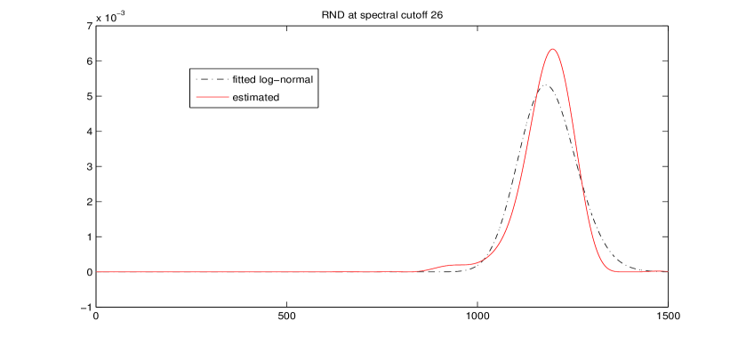
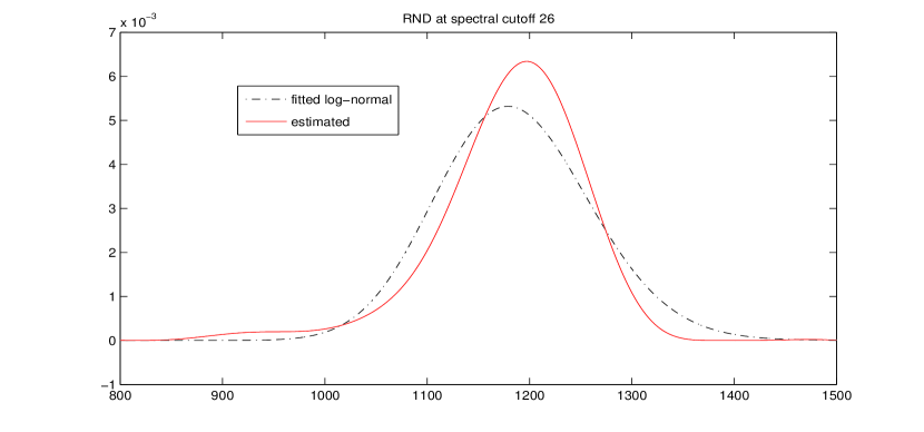
Figure 3: Here we plot the RND $q^{\bigstar}_{26}$ (solid line) estimated from the real price quotes reported in 1. We choose $B=1.4*F_{0}=1.4*S_{0}*e^{(r-\delta)\tau}=1660$ for that plot. In addition, we plot the best log-normal fit (in a least-square sense) to the average price quotes (dashed line). It is obtained for $\sigma_{opt}=0.143$. At the top, we display the full left tail of the RND $q^{\bigstar}_{26}$. At the bottom, we zoom in on the fat left tail of the estimated RND distribution.

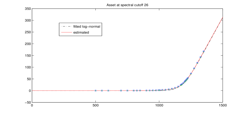
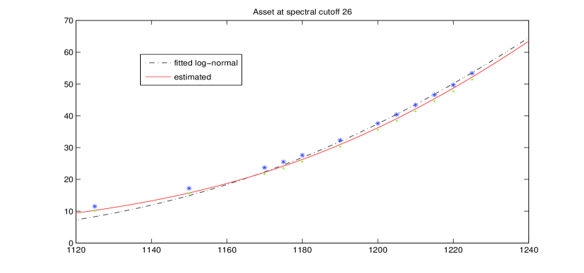
Figure 4: Here we plot the fitted put prices obtained from the setting described above in 3. The solid line corresponds to the fitted prices $P^{\bigstar}_{26}$, while the dashed line corresponds to the fitted prices obtained from a log-normal distribution. The stars and dots correspond to market ask and bid quotes, respectively. At the top, we give a large view of the fits. At the bottom we zoom in to show that $P^{\bigstar}_{26}$ lies inside the market quotes, while the fitted log-normal prices lie outside.

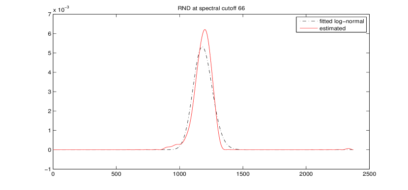
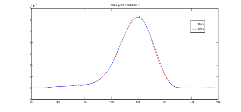
Figure 5: Here we plot the RND $q^{\bigstar}_{66}$ (solid line) estimated from the real price quotes reported in 1. We choose $B=2*F_{0}=2*S_{0}*e^{(r-\delta)\tau}=2372$ for that plot. In addition, we plot the best log-normal fit (in a least-square sense) to the average price quotes (dashed line). It is obtained for $\sigma_{opt}=0.143$. At the top, we display the full left tail of the RND $q^{\bigstar}_{66}$ and its full right tail up to $B$. At the bottom, we superimpose $q^{\bigstar}_{66}$ (solid line) with $q^{\bigstar}_{26}$ (dashed line) obtained in 3 for an other choice of $B$. Notice the strong agreement between both densities, which highlights the stability of the SRM with respect to the choice of $B$. Interestingly, $q^{\bigstar}_{66}$ is slightly more bumpy than $q^{\bigstar}_{26}$ at the level of its left fat-tail. This reinforces our argument that smoothness goes hand in hand with low spectral cutoff.

8.2 Simulated data

As regards the simulated data, we work in the Black-Scholes setting. In that context the price of a put option admits a closed form solution and the RND is log-normal (see Proposition 8.1). We model the bid-ask spread as a random noise around the true price given by the Black-Scholes formula. More precisely, for a given set of quoted strikes $\xi_{1}<\ldots<\xi_{s}$ and corresponding put prices $P(\xi_{1}),\ldots,P(\xi_{s})$, we write $y_{i}^{Ask}=P(\xi_{i})+z_{i}/2$ and $y_{i}^{Bid}=P(\xi_{i})-z_{i}/2$, where $z_{i}=\max(1,\min(3,\varpi|\xi_{i}|))$, the $\xi_{i}$’s are iid standard normal random variables and $\varpi=0.1\max_{1\leq i\leq s}P(\xi_{i})$. The bounds $1$ and $3$ are chosen by analogy with the real data quotes in 1. Of course, the bid-ask quotes we obtain in that way are not arbitrage free. However, they contain the true put price $P(\xi)$, which, given the nature of the quadratic program described in P1 above, is all that matters to approximate the true RND. For the sake of simplicity, we choose $r=0$, $\delta=0$, $\tau=1$, $S_{0}=100$, and $\sigma=0.3$ and $B=2*F_{0}=2*S_{0}$. In addition we set a first strike price at ${\lfloor F_{0}\rfloor}$ and spread the others on its left and right sides at unit length distance away from each other until we obtain $s$ strikes. More precisely, the second strike would be ${\lfloor F_{0}\rfloor}-1$, the third ${\lfloor F_{0}\rfloor}+1$, the fourth ${\lfloor F_{0}\rfloor}-2$ and so on and so forth. We plot the results for the first two spectral cutoffs at which a feasible point is found below in 6 in the case where there are as little as $s=5$ bid ask quotes and in 7 in the case where there are as many as $s=50$ of them. In any case, we can see that we obtain a smooth density that resembles the log-normal density generating the initial quoted prices and that the estimate is stable from one spectral cutoff to another. Of course, the more strikes we have, the better the fit. Besides, we observe as expected from an other simulation not reported here that, the smaller the bid-ask spread, the better the fit. Notice once again that the fitted right-tail reaches zero in $B$, while the true one is strictly positive at that point. As before, this is due to the fact that $\psi_{k}(B)=0$.

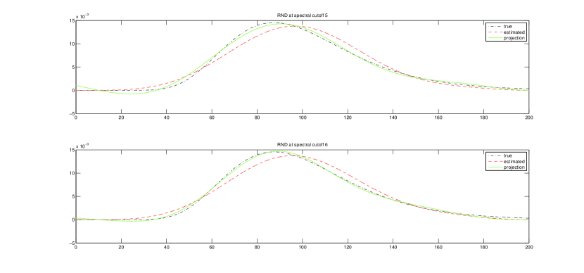
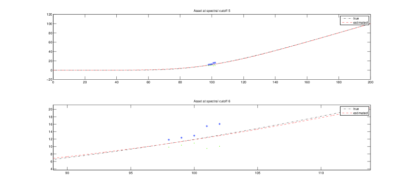
Figure 6: Here we are in the case of $5$ simulated bid ask quotes and with $B=2*F_{0}=200$. The first two plots display $q^{\bigstar}_{5}$ and $q^{\bigstar}_{6}$ (dashed line), the true log-normal RND used to generate the prices (dashed-dotted line) and the orthogonal projection of the true log-normal RND on $\{\psi_{0},\dots,\psi_{N}\}$ for $N=5$ and $N=6$ (solid line), respectively. The last two plots display the fitted put prices, that is $P_{5}^{\bigstar}$ and $P_{6}^{\bigstar}$ (dashed line) together with the true prices (dashed-dotted line).

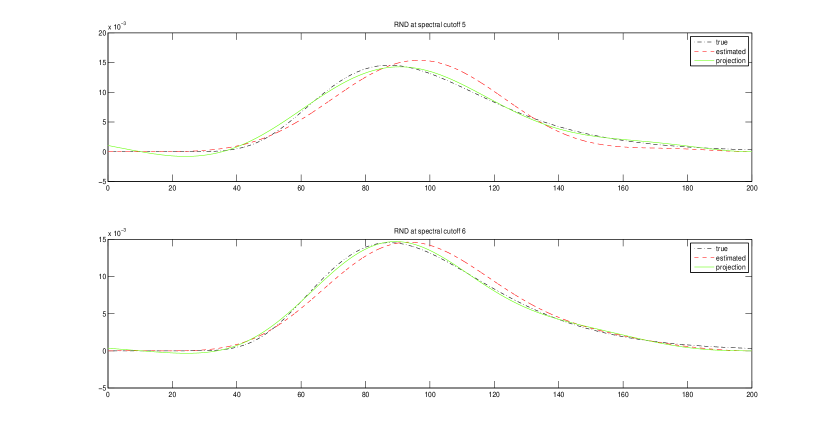
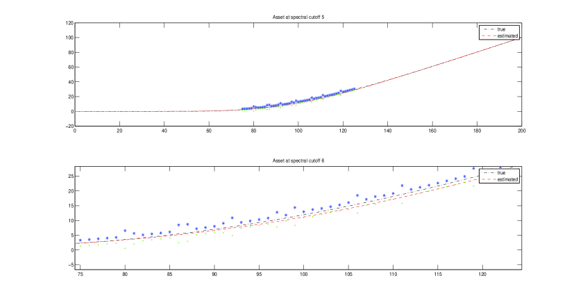
Figure 7: Here, we repeat the same plots as in 7 in the case of $50$ simulated bid-ask quotes.

Appendix

Refresher on the Black-Scholes model

This is a well-known result of mathematical finance.

Proposition 8.1.

Let us denote by $S_{0}$ the price today of a stock paying dividends continuously over time at a constant rate $\delta$ and by $r$ the continuously compounded risk-free rate. The arbitrage price today of a put option on that stock maturing at time $\tau$ is given by the following closed form formula,

$$P(\xi) =\xi e^{-r\tau}\mathcal{N}(-d_{2})-S_{0}e^{-\delta\tau}\mathcal{N}(-d_{1}),$$

with

$$d_{1} =\frac{\ln(S_{0}/\xi)+[(r-\delta)+\frac{1}{2}\sigma^{2}]\tau}{\sigma\sqrt{\tau}}, d_{2} =d_{1}-\sigma\sqrt{\tau},$$

where $\sigma$ stands for the volatility of the stock and $\mathcal{N}$ for the standard normal cumulative distribution. In addition, the RND is log-normal and writes as

$$q(x) =\frac{1}{\sqrt{2\pi}\sigma\tau x}\exp\left(-\frac{[\ln(x/S_{0})-(r-\delta)\tau+\frac{1}{2}\sigma^{2}\tau]^{2}}{2\sigma^{2}\tau}\right).$$

Proof.

These results can be found in see [21, p.117], for example. ∎

Additional results relative to $\gamma$ and $\gamma^{*}$

We now present three results relative to $\gamma$ and $\gamma^{*}$, which are either used in the core of the paper or of interest in their own right.

Proposition 8.2.

The operators $\gamma$ and $\gamma^{*}$ admit no eigenvectors.

Proof.

Suppose $f$ is an eigenvector of $\gamma$ associated to eigenvalue $\lambda$, then denote by

(8.1) $$\breve{f}(t)=f(B-\xi),$$

and notice that for all $\xi\in{\mathcal{I}}$, a direct application of Lemma 8.2 allows to write

$$\lambda\breve{f}(B-\xi)=\lambda f(\xi) =\gamma f(\xi)=\gamma^{*}\breve{f}(B-\xi).$$

Thus $\breve{f}$ must be an eigenvector of $\gamma^{*}$. However, it is well known that $\gamma^{*}$ admits no eigenvalue since, for any $\lambda\neq 0$,

$$\lambda f(\xi) =\gamma^{*}f(\xi)=\int_{0}^{\xi}\theta^{*}(\xi,x)f(x)dx, \xi\in{\mathcal{I}},$$

defines a homogeneous Volterra equation in $f$, whose unique trivial solution is $f=0$ (see [12, p.239, Th. 5.5.2]). ∎

Finally, let us point out the two following useful lemmas.

Lemma 8.1.

Let us denote by $\partial_{\xi}^{k}$ the $k^{th}$ order partial differential operator with respect to $\xi$. Then, for any $f\in\mathbb{L}_{2}{\mathcal{I}}$, we have the following results.

$$f =\partial_{\xi}^{2}\gamma f, f =\partial_{\xi}^{2}\gamma^{*}f,$$

$$f =\partial_{\xi}^{4}\gamma^{*}\gamma f, f =\partial_{\xi}^{4}\gamma\gamma^{*}f.$$

Proof.

Notice indeed that

$$\partial_{\xi}\gamma f(\xi) =\partial_{\xi}\int_{\xi}^{B}(x-\xi)f(x)dx=-\int_{\xi}^{B}f(x)dx,$$

$$\partial_{\xi}\gamma^{*}f(\xi) =\partial_{\xi}\int_{0}^{\xi}(\xi-x)f(x)dx=\int_{0}^{\xi}f(x)dx.$$

Therefore, we obtain immediately

$$f=\partial_{\xi}^{2}\gamma f=\partial_{\xi}^{2}\gamma^{*}f.$$

The remaining of the proof follows directly from these first results. Notice indeed that,

$$\partial_{\xi}^{4}\gamma^{*}\gamma f=\partial_{\xi}^{2}[\partial_{\xi}^{2}\gamma^{*}](\gamma f)=\partial_{\xi}^{2}\gamma f=f.$$

which concludes the proof. ∎

Lemma 8.2.

For any $f\in\mathbb{L}_{2}{\mathcal{I}}$ and $\xi\in{\mathcal{I}}$, we have $\gamma f(\xi)=\gamma^{*}\breve{f}(B-\xi)$ (see 8.1 for notations).

Proof.

Perform the change of variable $u=B-x$ to obtain

$$\gamma f(\xi) =\int_{\xi}^{B}(x-\xi)f(x)dx$$

$$=\int_{0}^{B-\xi}([B-\xi]-u)\breve{f}(u)du=\gamma^{*}\breve{f}(B-\xi).$$

∎

Relation between the $(\varphi_{k})$s and the $(\psi_{k})$s

We believe that $m_{0}(q)$ and $m_{1}(q)$ could be readily estimated from the data, so that 7.2 could be used to construct a second estimator of the RND based on the restricted call operator. This second estimator could eventually be combined with the one obtained from the SRM above. To that end, and for the sake of completeness, we compute the scalar products between elements of the two singular bases. Results are reported in the following proposition.

Proposition 8.3.

Let us write

$$\mathfrak{p}_{k,m}(x,y) =(-x^{3}+x^{2}y)(-1)^{m+k}-xy^{2}+y^{3},$$

$$\mathfrak{q}_{k,m}(x,y) =(x^{3}+x^{2}y)(-1)^{k}+(y^{3}+y^{2}x)(-1)^{m}.$$

Then, we have the following relationships,

$$\langle\varphi_{k},\psi_{m}\rangle$$

$$=4\frac{\mathfrak{p}_{k,m}(\rho_{k},\rho_{m})e^{-\rho_{k}-\rho_{m}}-\mathfrak{q}_{k,m}(\rho_{k},\rho_{m})e^{-\rho_{k}}+\mathfrak{q}_{k,m}(\rho_{m},\rho_{k})e^{-\rho_{m}}+\mathfrak{p}_{k,m}(\rho_{m},\rho_{k})}{(\rho_{k}^{4}-\rho_{m}^{4})(1+(-1)^{m}e^{-\rho_{m}})(1+(-1)^{k}e^{-\rho_{k}})},k\neq m,$$

$$\langle\varphi_{k},\psi_{k}\rangle =\frac{-e^{-2\rho_{k}}(\rho_{k}+2)+2\rho_{k}(-1)^{k}e^{-\rho_{k}}-\rho_{k}+2}{(e^{-\rho_{k}}+(-1)^{k})^{2}\rho_{k}}.$$

On the way, we obtain,

$$\langle h_{k,1},h_{m,1}\rangle$$

$$=((-1)^{k}+(-1)^{m})\frac{(\rho_{k}+\rho_{m})(e^{-\rho_{m}}-e^{-\rho_{k}})+(-1)^{k}(\rho_{k}-\rho_{m})(1-e^{-(\rho_{k}+\rho_{m})})}{(\rho_{k}^{2}-\rho_{m}^{2})(1+(-1)^{k}e^{-\rho_{k}})(1+(-1)^{m}e^{-\rho_{m}})},k\neq m,$$

$$\langle h_{k,1},h_{m,2}\rangle$$

$$=((-1)^{k}-(-1)^{m})\frac{(\rho_{k}+\rho_{m})(e^{-\rho_{m}}+e^{-\rho_{k}})-(-1)^{k}(\rho_{k}-\rho_{m})(1+e^{-(\rho_{k}+\rho_{m})})}{(\rho_{k}^{2}+\rho_{m}^{2})(1+(-1)^{m}e^{-\rho_{m}})(1+(-1)^{k}e^{-\rho_{k}})},k\neq m,$$

$$\langle h_{k,1},h_{k,1}\rangle =\frac{1-e^{-2\rho_{k}}+2(-1)^{k}\rho_{k}e^{-\rho_{k}}}{\rho_{k}((-1)^{k}+e^{-\rho_{k}})^{2}},$$

$$\langle h_{k,1},h_{k,2}\rangle =0,$$

$$\langle h_{k,2},h_{m,2}\rangle =\delta_{k,m}-\langle h_{k,1},h_{m,1}\rangle.$$

Proof.

Recall that, for all $k,m$, we have defined

$$h_{k,1} =a_{k,1}f_{k,1}+a_{k,2}f_{k,2}, h_{k,2} =a_{k,3}f_{k,3}+a_{k,4}f_{k,4},$$

$$\varphi_{k} =h_{k,1}+h_{k,2}, \psi_{k} =h_{k,1}-h_{k,2}.$$

Besides, we have that

$$\langle\varphi_{k},\varphi_{m}\rangle =\delta_{k,m}=\langle h_{k,1},h_{m,1}\rangle+\langle h_{k,2},h_{m,2}\rangle+\langle h_{k,1},h_{m,2}\rangle+\langle h_{k,2},h_{m,1}\rangle,$$

$$\langle\psi_{k},\psi_{m}\rangle =\delta_{k,m}=\langle h_{k,1},h_{m,1}\rangle+\langle h_{k,2},h_{m,2}\rangle-\langle h_{k,1},h_{m,2}\rangle-\langle h_{k,2},h_{m,1}\rangle.$$

Therefore, we obtain the following relationships,

$$\delta_{k,m} =\langle h_{k,1},h_{m,1}\rangle+\langle h_{k,2},h_{m,2}\rangle,$$

$$0 =\langle h_{k,1},h_{m,2}\rangle+\langle h_{k,2},h_{m,1}\rangle.$$

Which leads to

$$\langle\varphi_{k},\psi_{m}\rangle =\langle h_{k,1},h_{m,1}\rangle-\langle h_{k,2},h_{m,2}\rangle-\langle h_{k,1},h_{m,2}\rangle+\langle h_{k,2},h_{m,1}\rangle,$$

$$=2(\langle h_{k,1},h_{m,1}\rangle-\langle h_{k,1},h_{m,2}\rangle)-\delta_{k,m}.$$

Now, it remains to compute $\langle h_{k,1},h_{m,1}\rangle$ and $\langle h_{k,1},h_{m,2}\rangle$. The results follow from lengthy and tedious but straightforward computations and are therefore not reported here. ∎

From the RND $q$ of $S_{\tau}$ to the density of $\ln S_{\tau}$

Some authors have chosen to focus on the estimation of the density of $\log S_{\tau}$ rather than on the density of $S_{\tau}$ itself. Both densities relate by a simple transformation, as described in the following proposition. In our case, this transformation can be readily applied since the SRM returns an analytic expression for the estimated RND.

Proposition 8.4.

If $X$ admits $f(x)$ for density on $\mathbb{R}$, then $Y=\exp(X)$ admits $\tfrac{1}{y}f(\ln y)$ for density on $\mathbb{R}^{+}$. Conversely, if $Y$ admits $f(y)$ for density on $\mathbb{R}^{+}$, then $X=\ln(Y)$ admits $e^{x}f(e^{x})$ for density on $\mathbb{R}$.

References

- [1] Peter A. Abken, Dilip B. Madan, and Sailesh Ramamurtie, Estimation of risk-neutral densities by Hermite polynomial approximation: with an application to eurodollar futures options, Federal Reserve Bank of Atlanta, working paper no. 96-5, (1996).
- [2] Yacine Aït-Sahalia and Jefferson Duarte, Nonparametric option pricing under shape restrictions, J. Econometrics, 116 (2003), pp. 9–47.
- [3] Bhupinder Bahra, Implied risk-neutral probability density functions from option prices: theory and application, Bank of England, working paper no. 1368-5562, (1997).
- [4] Fischer Black and Myron Scholes, The pricing of options and corporate liabilities, J. Polit. Econ., 81 (1973), pp. 637–654.
- [5] Oleg Bondarenko, Estimation of risk-neutral densities using positive convolution approximation, J. Econometrics, 116 (2003), pp. 85–112.
- [6] Douglas T. Breeden and Robert H. Litzenberger, Prices of state-contingent claims implicit in option prices, J. Bus., 51 (1978), pp. 621–651.
- [7] Ruijun Bu and Kaddour Hadri, Estimating option implied risk-neutral densities using spline and hypergeometric functions, Econometrics J., 10 (2007), pp. 216–244.
- [8] Peter W. Buchen and Michael Kelly, The maximum entropy distribution of an asset inferred from option prices, J. Finan. Quant. Anal., 31 (1996), pp. 143–159.
- [9] Rama Cont, Beyond implied volatility: extracting information from option prices, in Econophysics: an emergent science, J. Kertész and I. Kondor, eds., Dordrecht, Kluwer, 1997.
- [10] John C. Cox and Stephen A. Ross, The valuation of options for alternative stochastic processes, Journal of Financial Economics, 3 (1976), pp. 145–146.
- [11] Mark H. A. Davis and David G. Hobson, The range of traded option prices, Math. Finance, 17 (2007), pp. 1–14.
- [12] Lokenath Debnath and Piotr Mikusiński, Introduction to Hilbert spaces with applications, Academic Press, 1990.
- [13] Heinz W. Engl, Martin Hanke, and Andreas Neubauer, Regularization of inverse problems, Kluwer Academic Publishers, 1996.
- [14] Stephen Figlewski, Estimating the implied risk neutral density for the U.S. market portfolio, in Volatility and time series econometrics: essays in honor of Robert F. Engle, Tim Bollerslev, Jeffrey R. Russel, and Mark Watson, eds., Oxford University Press, 2008.
- [15] Paul R. Halmos, What does the spectral theorem say?, Am. Math. Mon., 70 (1963), pp. 241–247.
- [16] Ludger Hentschel, Errors in implied volatility estimation, J. Finan. Quant. Anal., 38 (2003), pp. 779–810.
- [17] Jens Carsten Jackwerth, Option-implied risk neutral distributions and risk aversion, Research Foundation of AIMR (CFA Institute), 2004.
- [18] Jens Carsten Jackwerth and Mark Rubinstein, Recovering probability distributions from option prices, J. Finance, 51 (1996), pp. 1611–1631.
- [19] Robert Jarrow and Andrew Rudd, Approximate option valuation for arbitrary stochastic processes, J. Finan. Econ., 10 (1982), pp. 347–369.
- [20] Robert C. Merton, Theory of rational option pricing, Bell J. Econ. Manag. Sci., 4 (1973), pp. 141–183.
- [21] Marek Musiela and Marek Rutkowski, Martingale methods in financial modeling, ed., Springer-Verlag, 2008.
- [22] Marc Potters, Rama Cont, and Jean-Philippe Bouchaud, Financial markets as adaptive systems, Europhys. Lett., 41 (1998), pp. 239–244.
- [23] Michael Stutzer, A simple approach to derivative security valuation, J. Finance, 51 (1996), pp. 1633–1652.