On solvability and integrability of the Rabi model

Abstract

Quasi-exactly solvable Rabi model is investigated within the framework of the Bargmann Hilbert space of analytic functions ${\cal B}$. On applying the theory of orthogonal polynomials, the eigenvalue equation and eigenfunctions are shown to be determined in terms of three systems of monic orthogonal polynomials. The formal Schweber quantization criterion for an energy variable $x$, originally expressed in terms of infinite continued fractions, can be recast in terms of a meromorphic function $F(z)=a_{0}+\sum_{k=1}^{\infty}{\cal M}_{k}/(z-\xi_{k})$ in the complex plane $\mathbb{C}$ with real simple poles $\xi_{k}$ and positive residues ${\cal M}_{k}$. The zeros of $F(x)$ on the real axis determine the spectrum of the Rabi model. One obtains at once that, on the real axis, (i) $F(x)$ monotonically decreases from $+\infty$ to $-\infty$ between any two of its subsequent poles $\xi_{k}$ and $\xi_{k+1}$, (ii) there is exactly one zero of $F(x)$ for $x\in(\xi_{k},\xi_{k+1})$, and (iii) the spectrum corresponding to the zeros of $F(x)$ does not have any accumulation point. Additionally, one can provide much simpler proof of that the spectrum in each parity eigenspace ${\cal B}_{\pm}$ is necessarily nondegenerate. Thereby the calculation of spectra is greatly facilitated. Our results allow us to critically examine recent claims regarding solvability and integrability of the Rabi model.

I Introduction

The Rabi model Rb describes the simplest interaction between a cavity mode with a bare frequency $\omega$ and a two-level system with a bare resonance frequency $\omega_{0}$. The model is characterized by the Hamiltonian Rb ; Schw ; Br ; YZL

$$\hat{H}_{R}=\hbar\omega\mathds{1}\hat{a}^{\dagger}\hat{a}+\hbar g\sigma_{1}(\hat{a}^{\dagger}+\hat{a})+\mu\sigma_{3},$$ (1)

where $\mathds{1}$ is the unit matrix, $\hat{a}$ and $\hat{a}^{\dagger}$ are the conventional boson annihilation and creation operators satisfying commutation relation $[\hat{a},\hat{a}^{\dagger}]=1$, $g$ is a coupling constant, and $\mu=\hbar\omega_{0}/2$. In what follows we assume the standard representation of the Pauli matrices $\sigma_{j}$ and set the reduced Planck constant $\hbar=1$. For dimensionless coupling strength $\kappa=g/\omega\lesssim 10^{-2}$, the physics of the Rabi model is well captured by the analytically solvable approximate Jaynes and Cummings (JC) model JC ; SK . The latter is obtained from the former upon applying the rotating wave approximation (RWA), whereby the coupling term $\sigma_{1}(\hat{a}^{\dagger}+\hat{a})$ in Eq. (1) is replaced by $(\sigma_{+}\hat{a}+\sigma_{-}\hat{a}^{\dagger})$, where $\sigma_{\pm}\equiv(\sigma_{1}\pm i\sigma_{2})/2$. Nowdays, solid-state semiconductor KGK and superconductor systems BGA ; FLM ; NDH have allowed the advent of the ultrastrong coupling regime, where the dimensionless coupling strength $\kappa\gtrsim 0.1$ CC . In this regime, the validity of the RWA breaks down and the relevant physics can only be described by the full Rabi model Rb . With new experiments rapidly approaching the limit of the deep strong coupling regime characterized in that $\kappa\gtrsim 1$ CRL , i.e., an order of magnitude stronger coupling, the relevance of the Rabi model Rb becomes even more prominent. There is every reason to believe that ultrastrong and deep strong coupling systems could open up a rich vein of research on truly quantum effects with implications for quantum information science and fundamental quantum optics KGK .

The Rabi model applies to a great variety of physical systems, including cavity and circuit quantum electrodynamics, quantum dots, polaronic physics and trapped ions. In spite of recent claims Br ; Sln , the model is not exactly solvable. Rather it is a typical example of quasi-exactly solvable (QES) models in quantum mechanics TU ; Trb ; BD ; KUW ; KKT . The QES models are distinguished by the fact that a finite number of their eigenvalues and corresponding eigenfunctions can be determined algebraically TU ; Trb ; BD ; KUW . That is also the case of the Rabi model KKT . Certain energy levels of the Rabi model, known as Juddian exact isolated solutions Jd , can be analytically computed Jd ; Ks ; KL , whereas the remaining part of the spectrum not Ks ; KL . Depending on model parameters, the spectrum can only be approximated (sometime rather accurately - cf. Eqs. (18), (20) and Fig. 3 of Ref. FKU ; Eq. (20) and Figs. 1,2 of Ref. Ir ). Therefore, any kind of exact results involving the Rabi model continues to be of great theoretical and experimental value.

In our earlier work AMep we studied the Rabi model as a member of a more general class ${\cal R}$ of quantum models. In the Hilbert space ${\cal B}=L^{2}(\mathbb{R})\otimes\mathbb{C}^{2}$, where $L^{2}(\mathbb{R})$ is represented by the Bargmann space of entire functions $\mathfrak{b}$, and $\mathbb{C}^{2}$ stands for a spin space Schw ; Brg , the models of the class ${\cal R}$ were characterized in that the eigenvalue equation

$$\hat{H}\Phi=E\Phi,$$ (2)

where $\hat{H}$ denotes a corresponding Hamiltonian, reduces to a three-term difference equation

$$\phi_{n+1}+a_{n}\phi_{n}+b_{n}\phi_{n-1}=0\hskip 34.14322pt(n\geq 0).$$ (3)

Here $\{\phi_{n}\}_{n=0}^{\infty}$ are the sought expansion coefficients of an entire function

$$\upvarphi(z)=\sum_{n=0}^{\infty}\phi_{n}z^{n}$$ (4)

in $\mathfrak{b}$ that generates a physical state $\Phi(z)$ (in general vector in a spin space - see below). Models of the class ${\cal R}$ were then characterized in that the recurrence coefficients have an asymptotic powerlike dependence AMep

$$a_{n}\sim an^{\varsigma},\leavevmode\nobreak\ \leavevmode\nobreak\ \leavevmode\nobreak\ \leavevmode\nobreak\ \leavevmode\nobreak\ \leavevmode\nobreak\ \leavevmode\nobreak\ \leavevmode\nobreak\ \leavevmode\nobreak\ \leavevmode\nobreak\ \leavevmode\nobreak\ b_{n}\sim bn^{\upsilon}\hskip 34.14322pt(n\rightarrow\infty),$$ (5)

where $a$ and $b$ are proportionality constants and the exponents satisfy $2\varsigma>\upsilon$ and $\tau=\varsigma-\upsilon\geq 1/2$ AMep . In virtue of the Perron and Kreuser generalizations (Theorems 2.2 and 2.3(a) in Ref. Gt ) of the Poincaré theorem (Theorem 2.1 in Ref. Gt ), the recurrence equation (3) (considered for $n\geq 1$) possesses two linearly independent solutions:

• (i) a dominant solution $\{d_{j}\}_{j=0}^{\infty}$ and

• (ii) a minimal solution $\{m_{j}\}_{j=0}^{\infty}$.

The respective solutions differ in the behavior $\phi_{n+1}/\phi_{n}$ in the limit $n\rightarrow\infty$. The minimal solution guaranteed by the Perron-Kreuser theorem (Theorem 2.3 in Ref. Gt ) for models of the class ${\cal R}$ satisfies

$$\frac{m_{n+1}}{m_{n}}\sim-\frac{b}{a}\frac{1}{n^{\tau}}\rightarrow 0\hskip 34.14322pt(n\rightarrow\infty)$$ (6)

in virtue of (5) and $\tau\geq 1/2>0$. On substituting the minimal solution for the $\phi_{n}$’s in Eq. (4), $\upvarphi(z)$ automatically becomes an entire function belonging to $\mathfrak{b}$ AMep . In what follows, only the minimal solutions will be considered, and $\upvarphi(z)$ in Eq. (4) will stand for the entire function generated by the minimal solution [of the $n\geq 1$ part of Eq. (3)].

The spectrum of any quantum model of ${\cal R}$ can be obtained as zeros of the transcendental function of a dimensionless energy parameter $x$ AMep ; AMcm ,

$$F(x)\equiv a_{0}+\sum_{k=1}^{\infty}\rho_{1}\rho_{2}\ldots\rho_{k},$$ (7)

where $F(x)$ is defined solely in terms of the coefficients of the three-term recurrence AMep ; AMcm ; AMr :

$$\rho_{1} = -\frac{b_{1}}{a_{1}},\hskip 8.5359pt\rho_{l}=u_{l}-1,\hskip 8.5359ptu_{1}=1,$$

$$u_{l} = \frac{1}{1-u_{l-1}b_{l}/(a_{l}a_{l-1})},\hskip 8.5359ptl\geq 2.$$ (8)

The function $F(x)$ yields both analytic and efficient numerical representation of the formal Schweber quantization criterion expressed in terms of infinite continued fractions (cf. Eq. (A.16) of Ref. Schw ),

$$0=F(x)\equiv a_{0}+\frac{-b_{1}}{a_{1}-}\frac{b_{2}}{a_{2}-}\frac{b_{3}}{a_{3}-}\cdots$$ (9)

The condition $F(x)=0$ is equivalent to that the logarithmic derivative of $\upvarphi(z)$ satisfies the boundary condition

$$r_{0}\equiv\frac{\upvarphi^{\prime}(0)}{\upvarphi(0)}=-a_{0},$$ (10)

where $r_{0}$ stands for the infinite continued fraction on the right-hand side in Eq. (9) AMep . An important insight missed in Refs. Schw ; AMep is that the spectrum of any quantum model of ${\cal R}$ is necessarily nondegenerate, unless the conditions that guarantee uniqueness of the minimal solution the recurrence (3) cannot be satisfied (cf. Sec. V.2).

The Rabi Hamiltonian $\hat{H}_{R}$ is known to possess a discrete $\mathbb{Z}_{2}$-symmetry corresponding to the constant of motion, or parity, $\hat{\Pi}=\exp(i\pi\hat{J})$ Br ; CRL ; Ks , where

$$\hat{J}=\mathds{1}\hat{a}^{\dagger}\hat{a}+\frac{1}{2}\,(\mathds{1}+\sigma_{3})$$ (11)

is the familiar operator known to generate a continuous $U(1)$ symmetry of the JC model Br ; JC . In order to employ the Fulton and Gouterman reduction FG in the positive and negative parity spaces, wherein one component of $\Phi$ is generated from the other by means of a suitable cyclic operator $\hat{\gamma}$, $\hat{\gamma}^{2}=1$, it is expedient to work in a unitary equivalent single-mode spin-boson picture

$$\hat{H}_{sb}=\omega\mathds{1}\hat{a}^{\dagger}\hat{a}+\mu\sigma_{1}+g\sigma_{3}(\hat{a}^{\dagger}+\hat{a}).$$

The transformation is accomplished by means of the unitary operator $U=(\sigma_{1}+\sigma_{3})/\sqrt{2}=U^{-1}$. Hamiltonian $\hat{H}_{sb}$ is then of the Fulton and Gouterman type (see Sec. IV of Ref. FG )

$$\hat{H}_{FG}=A\mathds{1}+B\sigma_{1}+C\sigma_{3},$$

with

$$A=\omega\hat{a}^{\dagger}\hat{a},\leavevmode\nobreak\ \leavevmode\nobreak\ \leavevmode\nobreak\ \leavevmode\nobreak\ \leavevmode\nobreak\ B=\mu,\leavevmode\nobreak\ \leavevmode\nobreak\ \leavevmode\nobreak\ \leavevmode\nobreak\ \leavevmode\nobreak\ C=g(\hat{a}^{\dagger}+\hat{a}).$$

The Fulton and Gouterman symmetry operation is realized by $\hat{\gamma}=e^{i\pi\hat{a}^{\dagger}\hat{a}}$, which transforms a given operator $\hat{O}$ according to

$$\hat{O}\rightarrow e^{i\pi\hat{a}^{\dagger}\hat{a}}\hat{O}e^{-i\pi\hat{a}^{\dagger}\hat{a}}.$$

The latter induces reflections of the annihilation and creation operators: $\hat{a}\rightarrow-\hat{a}$, $\hat{a}^{\dagger}\rightarrow-\hat{a}^{\dagger}$, and leaves the boson number operator $\hat{a}^{\dagger}\hat{a}$ invariant Br ; FG . Because $[\hat{\gamma},A]=[\hat{\gamma},B]=\{\hat{\gamma},C\}=0$, $\hat{\Pi}_{FG}=\sigma_{1}\hat{\gamma}$ is the symmetry of $\hat{H}_{sb}$ Br ; FG . One can verify that, with $\sigma_{3}$ replaced by $\sigma_{1}$ in Eq. (11),

$$\hat{\Pi}=e^{i\pi\hat{J}}=-\sigma_{1}e^{i\pi\hat{a}^{\dagger}\hat{a}}=-\sigma_{1}\hat{\gamma}=-\hat{\Pi}_{FG}.$$

Such as to any cyclic $\mathbb{Z}_{2}$ operator, one can associate to $\hat{\Pi}_{FG}$ a pair of projection operators

$$P^{\pm}=\frac{1}{2}\,(\mathds{1}\pm\hat{\Pi}_{FG}),\leavevmode\nobreak\ \leavevmode\nobreak\ \leavevmode\nobreak\ \leavevmode\nobreak\ \leavevmode\nobreak\ \left(P^{\pm}\right)^{2}=P^{\pm}.$$

The respective projection operators $P^{\pm}$ project out eigenstates of $\hat{\Pi}_{FG}$: an arbitrary state $\Psi\in{\cal B}$ is projected into corresponding parity eigenstates $\Phi^{\pm}$ with positive and negative parity. In the conventional off-diagonal Pauli representation of $\sigma_{1}$ one has FG :

$$P^{+}\Psi=\frac{1}{2}\,\left(\begin{array}[]{cc}1&\hat{\gamma}\\ \hat{\gamma}&1\end{array}\right)\left(\begin{array}[]{c}\uppsi_{1}\\ \uppsi_{2}\end{array}\right)=\frac{1}{2}\,\left(\begin{array}[]{c}\uppsi_{1}+\hat{\gamma}\uppsi_{2}\\ \hat{\gamma}(\uppsi_{1}+\hat{\gamma}\uppsi_{2})\end{array}\right).$$ (12)

The right-hand side of Eq. (12) shows that one component of the positive parity eigenstate can be generated from the other by means of the symmetry operator $\hat{\gamma}$ FG . A similar argument holds for $P^{-}$, wherein $-\hat{\gamma}$ is substituted for $\hat{\gamma}$ in Eq. (12). Therefore, the corresponding parity eigenstates $\Phi^{+}$ and $\Phi^{-}$ of the eigenvalue equation (2) contain one independent component each,

$$\Phi^{+}(z)=\left(\begin{array}[]{c}\upvarphi^{+}\\ \hat{\gamma}\upvarphi^{+}\end{array}\right),\hskip 22.76228pt\Phi^{-}(z)=\left(\begin{array}[]{c}\upvarphi^{-}\\ -\hat{\gamma}\upvarphi^{-}\end{array}\right).$$ (13)

For the sake of comparison with Ref. Br , the superscript $\pm$ denotes the positive and negative parity states of $\hat{\Pi}_{FG}$ and not of the conventional parity operator $\hat{\Pi}$.

The respective parity eigenstates $\Phi^{+}(z)$ and $\Phi^{-}(z)$ satisfy the following eigenvalue equations for the independent (e.g. upper) component (cf. Eqs. (4.12-13) of Ref. FG )

$$H^{+}\upvarphi^{+} = [A+B\hat{\gamma}+C]\upvarphi^{+}=E^{+}\upvarphi^{+},$$

$$H^{-}\upvarphi^{-} = [A-B\hat{\gamma}+C]\upvarphi^{-}=E^{-}\upvarphi^{-}.$$

Here we have written $E^{\pm}$ since, in general, the spectra of $H^{+}$ and $H^{-}$ do not coincide. In the Bargmann space of entire functions $\mathfrak{b}$, the action of $\hat{\gamma}$ becomes AMep

$$\hat{\gamma}\upvarphi^{\pm}(z)=\upvarphi^{\pm}(-z)=\sum_{n=0}^{\infty}(-1)^{n}\phi_{n}^{\pm}z^{n}.$$

Therefore, the Rabi model can be characterized by a pair of the three-term recurrences (Eq. (37) of Ref. AMep )

$$\phi_{n+1}^{\pm}+\frac{1}{\kappa(n+1)}\,[n-\upepsilon\pm(-1)^{n}\Delta]\phi_{n}^{\pm}$$ (14)

$$+\frac{1}{n+1}\,\phi_{n-1}^{\pm}=0,$$

where $\upepsilon\equiv E^{\pm}/\omega$, $\kappa=g/\omega$ reflects the coupling strength, and $\Delta=\mu/\omega=\omega_{0}/(2\omega)$ AMep . The Hilbert space ${\cal B}=\mathfrak{b}\otimes\mathbb{C}^{2}$ can be thus written as a direct sum ${\cal B}={\cal B}_{+}\oplus{\cal B}_{-}$ of the parity eigenspaces. The case of a displaced harmonic oscillator, which is the exactly solvable limit of $\hat{H}_{R}$ for $\mu=0$, corresponds to $\Delta=0$, whereby the recurrence (14) reduces to Eq. (A.17) of Ref. Schw . Because the recurrence (14) satisfies the conditions that guarantee uniqueness of the minimal solution, i.e. each $\upvarphi^{\pm}(z)$ generated by the respective minimal solutions is unique, the spectrum in each parity eigenspace ${\cal B}_{\pm}$ is necessarily nondegenerate (cf. Sec. V.2).

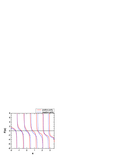
Figure 1: $F(x)$ corresponding to the recurrence (14) of the Rabi model in the deep strong coupling regime for $\kappa=1.4$, $\Delta=0.4$, $\omega=1$, and $x=\upepsilon/\kappa=E/g$. Zeros of $F(x)$ determine the spectrum of the Rabi model in the respective parity subspaces ${\cal B}_{\pm}$. Parity is classified according to the sign of the eigenvalues of the parity operator $\hat{\Pi}_{FG}$.

In what follows, section II provides an overview of our main results. The results are proven in the forthcoming section III, which is divided into two subsections. First, subsection III.1 deal with the case of an arbitrary large but finite $n=N$. The limit $N\rightarrow\infty$ is then considered in subsection III.2. Section IV illustrates some of our findings on the exactly solvable case of the displaced harmonic oscillator. In Sec. V our results are then extensively discussed from various angles. Subsection V.1 gives a comparison of the properties of our $F$ with those of Braak’s functions $G_{\pm}$ and critically examines his integrability arguments. Subsection V.2 shows on a number of examples that the present approach is a powerful alternative to the Frobenius analysis Frb . Compared to the latter, it enables one an immediate insight regarding the nondegeneracy of the spectrum simply by checking that the conditions which guarantee uniqueness of the minimal solution are satisfied. In subsection V.3 recent claims regarding solvability of the Rabi model Br ; Sln are critically examined. A relation between the zeros of $\phi_{n}$ and the spectrum is discussed in subsection V.4. Compatibility of our results with some other results of the theory of infinite continued fractions and complex analysis is demonstrated in subsection V.5. Subsection V.6 gives an overview of some open problems. We then conclude with Sec. VI. Some additional technical remarks are relegated to Appendix A.

II Overview of the main results

In the case of the Rabi model, and its special case of the displaced harmonic oscillator, it was observed that the plots of $F(\upepsilon)$ corresponding to (14) displayed a series of discontinuous branches monotonically decreasing between $+\infty$ and $-\infty$ (see Fig. 1 and Figs. 1,2 of Ref. AMep ). In the present work the latter property will be proven. First we show that $F(x)$, considered as a function of $x\equiv\upepsilon/\kappa=E^{\pm}/g$, can be alternatively expressed as the limit of rational functions

$$F(x)\equiv\lim_{n\rightarrow\infty}F_{n}(x)=a_{0}+\lim_{n\rightarrow\infty}\frac{P_{n-1}^{(1)}(x)}{P_{n}(x)},$$ (15)

where $\{P_{n}(x)\}$ and $\{P_{n}^{(1)}(x)\}$ are associated systems of monic orthogonal polynomials. (Monic means here that the coefficient of the highest power of $x$ is one.) For $n\geq 1$, the polynomials of each orthogonal polynomial system (OPS) $\{P_{n}(x)\}$ and $\{P_{n}^{(1)}(x)\}$

• have real and simple zeros, and

• the zeros of $P_{n-1}^{(1)}(x)$ and $P_{n}(x)$ are interlaced.

Specifically, denote the zeros of $P_{n}(x)$ with degree $P_{n}=n$ by $x_{n1}<x_{n2}<\ldots<x_{nn}$ and the zeros of $P_{n-1}^{(1)}(x)$ with degree $n-1$ by $x_{n-1,1}^{(1)}<x_{n-1,2}^{(1)}<\ldots<x_{n-1,n-1}^{(1)}$. Then for any $k=1,2,\ldots,n-1$

$$x_{n,k}^{(\alpha)}<x_{n-1,k}^{(\alpha)}<x_{n,k+1}^{(\alpha)},$$ (16)

$$x_{nk}<x_{n-1,k}^{(1)}<x_{n,k+1},$$ (17)

where $\alpha=0,1$ (for the sake of notation the superscript $(0)$ for $\alpha=0$ will be suppressed in what follows). For each fixed $k$, $\{x_{nk}\}_{n=k}^{\infty}$ is a decreasing sequence and the limit

$$\xi_{k}=\lim_{n\rightarrow\infty}x_{nk}$$ (18)

exists. Additionally, for any finite $n$ the ratio in (15), also known as a convergent, enables a partial fraction decomposition (PFD)

$$\frac{P_{n-1}^{(1)}(x)}{P_{n}(x)}=\sum_{k=1}^{n}\frac{M_{nk}}{x-x_{nk}}\cdot$$ (19)

The numbers $M_{nk}$ are all positive, $M_{nk}>0$, and satisfy the condition

$$\sum_{k=1}^{n}M_{nk}=1.$$ (20)

Each number $M_{nk}$ can be shown to correspond to the weight corresponding to the zero $x_{nk}$ in the Gauss quadrature formula for the positive definite moment functional ${\cal L}$ associated with the OPS $\{P_{n}(x)\}$. In the case of the displaced harmonic oscillator and the Rabi model,

$$M_{nk} = -\frac{(n+1)!}{P_{n+1}(x_{nk})P_{n}^{\prime}(x_{nk})}$$ (21)

$$= \left(\sum_{l=0}^{n-1}\frac{P_{l}^{2}(x_{nk})}{(l+1)!}\right)^{-1}>0.$$

From (19) one finds immediately that whenever the derivative $dF_{n}(x)/dx$ exists, then

$$\frac{dF_{n}(x)}{dx}<0.$$ (22)

Consequently, between any two subsequent $x_{nk}<x_{n,k+1}$, where $F_{n}(x)$ decreases from $+\infty$ to $-\infty$, there is exactly one zero of $F_{n}(x)$, in agreement with Fig. 1 and Figs. 1,2 of Ref. AMep . $F_{n}(x)$ has its zeros and poles interlaced on the real axis. Now the coefficient

$$a_{0}=-x\pm(\Delta/\kappa)$$ (23)

is nonsingular. Because for $x>x_{0}=\pm(\Delta/\kappa)$ one has $a_{0}<0$, the PFD (19) and Eq. (17) imply that any two subsequent zeros $\{Z_{l}\}$ of $F_{n}(x)$ are interlaced for $Z_{l}>x_{0}$ as follows

$$x_{nl}<Z_{l}<x_{n-1,l}^{(1)}<x_{n,l+1}<Z_{l+1}.$$ (24)

For the zeros $Z_{l}\leq x_{0}$ one has $a_{0}>0$ and

$$Z_{0}<x_{n1}<x_{n-1,1}^{(1)}<Z_{1}<x_{n,2}<x_{n-1,2}^{(1)}<Z_{2}\ldots$$ (25)

At the crossover from positive to negative $a_{0}$ then

$$x_{n-1,l_{0}}^{(1)}<Z_{l_{0}}<x_{n,l_{0}+1}<Z_{l_{0}+1}<x_{n-1,l_{0}+1}^{(1)}$$ (26)

for some $l_{0}$. Thereby the above sharp inequalities prevent any accumulation point of the spectrum. That would also conclude any numerical method of computing $F(x)$ through Eq. (15), because of an unavoidable cutoff at some $n=N\gg 1$.

The above conclusions remain valid also in the limit $n\rightarrow\infty$. A point of crucial importance is that the inequality (16) survives the limit as the sharp inequality

$$\xi_{k}<\xi_{k+1}$$ (27)

for all $k\geq 1$. The sequence in Eq. (15) converges to a Mittag-Leffler PFD,

$$F(z)=a_{0}+\sum_{k=1}^{\infty}\frac{{\cal M}_{k}}{z-\xi_{k}},$$ (28)

defining a meromorphic function in the complex plane $\mathbb{C}$ with real simple poles and positive residues

$$0<{\cal M}_{k}=\left[\sum_{l=0}^{\infty}\frac{P_{l}^{2}(\xi_{k})}{(l+1)!}\right]^{-1}.$$ (29)

The series is absolutely and uniformly convergent in any finite domain having a finite distance from the simple poles $\xi_{j}$, and it defines there a holomorphic function of $z$ [$z\in\mathbb{C}$ here and below has no relation to $z$ in Eq. (4)]. One obtains at once that

$$\frac{dF(x)}{dx}<0.$$ (30)

Because $F(x)$ monotonically decreases from $+\infty$ to $-\infty$ between any its subsequent poles $\xi_{k}$ and $\xi_{k+1}$, there is exactly one zero of $F(x)$ for $x\in(\xi_{k},\xi_{k+1})$. As a byproduct, the spectrum in each parity eigenspace ${\cal B}_{\pm}$ does not have any accumulation point. Eventually, the knowledge of another OPS, $\{P_{n}^{(-1)}(x)\}$, enables one to determine the expansion coefficients of a physical state described by Eq. (4) as

$$\phi_{n}(x)=\frac{P_{n}^{(-1)}(x)}{n!}\cdot$$ (31)

III Proof of the main results

According to the Wallis formulas (Eqs. (III.2.1) of Ref. Chi ; Eqs. (4.2-3) of Ref. Gt ), given a three-term recurrence (3), the infinite continued fraction in Eq. (9) can be recast as the limit

$$r_{0}=\lim_{n\rightarrow\infty}\frac{A_{n}}{B_{n}}\cdot$$ (32)

Here the $n$th partial numerator $A_{n}$ and the $n$th partial denominator $B_{n}$ are determined as linearly independent solutions of the recurrence

$$A_{n} = a_{n}A_{n-1}-b_{n}A_{n-2},$$ (33)

$$B_{n} = a_{n}B_{n-1}-b_{n}B_{n-2},$$ (34)

where $n\geq 1$. The $A_{n}$’s and $B_{n}$’s are differentiated by the initial conditions:

$$A_{-1}=1,\leavevmode\nobreak\ \leavevmode\nobreak\ \leavevmode\nobreak\ \leavevmode\nobreak\ A_{0}=0,\leavevmode\nobreak\ \leavevmode\nobreak\ \leavevmode\nobreak\ \leavevmode\nobreak\ B_{-1}=0,\leavevmode\nobreak\ \leavevmode\nobreak\ \leavevmode\nobreak\ \leavevmode\nobreak\ B_{0}=1.$$ (35)

In an intriguing and peculiar world of infinite continued fractions, the respective recurrences (33) and (34) are essentially identical to the initial three-term recurrence (3) (up to the change $a_{n}\rightarrow-a_{n}$ and the omission of the $n=0$ term). For the Rabi model we have (Eq. (37) of Ref. AMep , or Eq. (14) herein above)

$$a_{n} = -\frac{1}{(n+1)}\,\left(\frac{\upepsilon}{\kappa}-\bar{c}_{n}\right),\leavevmode\nobreak\ \leavevmode\nobreak\ \leavevmode\nobreak\ \leavevmode\nobreak\ \leavevmode\nobreak\ b_{n}=\frac{1}{n+1},$$ (36)

$$\bar{c}_{n} \equiv \frac{1}{\kappa}\,[n\pm(-1)^{n}\Delta].$$ (37)

III.1 Arbitrary large but finite $N$

In order to prove the properties of $F_{n}(x)$ defined by Eq. (15) for an arbitrary $n$, together with the properties listed below, it is sufficient to prove that each of the recurrences (14), (33), (34) can be transformed into a recurrence of the type

$$P_{n}(x) = (x-c_{n})P_{n-1}(x)-\lambda_{n}P_{n-2}(x),$$ (38)

$$P_{-1}(x) = 0,\leavevmode\nobreak\ \leavevmode\nobreak\ \leavevmode\nobreak\ \leavevmode\nobreak\ \leavevmode\nobreak\ \leavevmode\nobreak\ P_{0}(x)=1,$$ (39)

where $n\geq 1$, the coefficients $c_{n}$ and $\lambda_{n}$ are real and independent of $x$, and $\lambda_{n}>0$. Obviously, the above recurrence defines a family of polynomials $\{P_{n}\}$ with degree $P_{n}=n$. According to Favard-Shohat-Natanson theorems (given as Theorems I-4.1 and I-4.4 of Ref. Chi ), satisfying the above recurrence is a necessary and sufficient condition that there exists a unique positive definite moment functional ${\cal L}$, such that for the family of polynomials $\{P_{n}\}$ holds

$${\cal L}[1]=\lambda_{1},\leavevmode\nobreak\ \leavevmode\nobreak\ \leavevmode\nobreak\ \leavevmode\nobreak\ \leavevmode\nobreak\ {\cal L}[P_{m}(x)P_{n}(x)]=\lambda_{1}\lambda_{2}\ldots\lambda_{n+1}\delta_{mn},$$ (40)

$m,n=0,1,2,\ldots$ and $\delta_{mn}$ is the Kronecker symbol. Thereby the polynomials $\{P_{n}\}$ form an OPS genr . Because $\lambda_{n}>0$, the norm of the polynomials $P_{n}$ is positive definite, ${\cal L}[P_{n}^{2}(x)]>0$, and ${\cal L}$ is positive definite moment functional (p. 16 of Ref. Chi ).

With $a_{n}$ and $b_{n}$ as in Eqs. (36), the substitution $B_{n}=(-1)^{n}P_{n}/(n+1)!$ transforms the three-term recurrence (34) into the recurrence of the type (38) and (39) with

$$c_{n}=\bar{c}_{n},\leavevmode\nobreak\ \leavevmode\nobreak\ \leavevmode\nobreak\ \leavevmode\nobreak\ \leavevmode\nobreak\ \lambda_{n}=\bar{\lambda}_{n}\equiv n,$$ (41)

where $\bar{c}_{n}$ has been defined by Eq. (37) and $x=\upepsilon/\kappa=E/g$. A similar substitution $A_{n}=(-1)^{n}S_{n}/(n+1)!$ transforms (33) into the recurrence

$$S_{n}(x)=(x-\bar{c}_{n})S_{n-1}-\lambda_{n}S_{n-2}$$ (42)

with $\lambda_{n}=n$, but with a “wrong” initial condition

$$S_{-1}=-1,\leavevmode\nobreak\ \leavevmode\nobreak\ \leavevmode\nobreak\ \leavevmode\nobreak\ S_{0}=0.$$ (43)

The latter is not of the required type (39). Note that a recurrence of the type (42) yields

$$S_{1} = \lambda_{1},$$

$$S_{2} = (x-\bar{c}_{2})\lambda_{1},$$

$$S_{3} = (x-\bar{c}_{3})(x-\bar{c}_{2})\lambda_{1}+\lambda_{3}\lambda_{1},$$

$$S_{3} = (x-\bar{c}_{4})(x-\bar{c}_{3})(x-\bar{c}_{2})\lambda_{1}+(x-\bar{c}_{4})\lambda_{3}\lambda_{1}$$ (44)

$$\leavevmode\nobreak\ \leavevmode\nobreak\ \leavevmode\nobreak\ \leavevmode\nobreak\ \leavevmode\nobreak\ \leavevmode\nobreak\ +(x-\bar{c}_{2})\lambda_{4}\lambda_{1},$$

$$\ldots$$

Therefore, a further substitution $S_{n}=\lambda_{1}Q_{n-1}$ transforms the recurrence (42) into

$$Q_{n}(x)=(x-\bar{c}_{n+1})Q_{n-1}(x)-\lambda_{n+1}Q_{n-2}(x),$$ (45)

where $n\geq 1$, with the “correct” initial conditions

$$Q_{-1}=0,\leavevmode\nobreak\ \leavevmode\nobreak\ \leavevmode\nobreak\ \leavevmode\nobreak\ Q_{0}=1.$$ (46)

The recurrence (45) together with the initial conditions is now of the type (38) and (39) with

$$c_{n}=\bar{c}_{n+1},\leavevmode\nobreak\ \leavevmode\nobreak\ \leavevmode\nobreak\ \leavevmode\nobreak\ \leavevmode\nobreak\ \lambda_{n}=\bar{\lambda}_{n+1}=n+1.$$ (47)

Eventually, the substitution $\phi_{n}\rightarrow\bar{\phi}_{n}/n!$ transforms the initial recurrence (14) into

$$\bar{\phi}_{n+1}^{\pm}=(x-\bar{c}_{n})\bar{\phi}_{n}^{\pm}-\bar{\lambda}_{n}\,\bar{\phi}_{n-1}^{\pm}.$$ (48)

The recurrence for $\bar{\phi}_{n}^{\pm}$ is again of the type (38) and (39) with

$$c_{n}=\bar{c}_{n-1},\leavevmode\nobreak\ \leavevmode\nobreak\ \leavevmode\nobreak\ \lambda_{n}=\bar{\lambda}_{n-1}=n-1,$$ (49)

where we set $\lambda_{1}=\bar{\lambda}_{0}=1\neq 0$ for $n=1$. Note in passing that $\lambda_{1}$ enters the recurrence (38) only in the product $\lambda_{1}P_{-1}$, where $P_{-1}$ satisfies the initial condition (39). Therefore we have the freedom to set $\lambda_{1}$ at our will. The initial conditions (39) in the case of the recurrence (48) for $\bar{\phi}_{n}^{\pm}$ are justified, because the logarithmic derivative of the entire function $\upvarphi(z)$ generated by the minimal solution (of the $n\geq 1$ part) of (3) satisfies the boundary condition (10). Combined with the fact that in the case of the recurrence (14) the coefficient $a_{0}$ is nonsingular [cf. Eq. (23)], one has necessary $\bar{\phi}_{0}^{\pm}\neq 0$. A suitable rescaling, which can be absorbed into an overall normalization prefactor, then always achieves $\bar{\phi}_{0}^{\pm}=1$.

Now the respective recurrences for $\bar{\phi}_{n}$’s, $P_{n}$’s, and $Q_{n}$’s have all been shown to be of the type

$$P_{n}^{(\alpha)}(x) = (x-\bar{c}_{n+\alpha})P_{n-1}^{(\alpha)}(x)-\bar{\lambda}_{n+\alpha}P_{n-2}^{(\alpha)}(x),$$ (50)

$$P_{-1}^{(\alpha)}(x) = 0,\leavevmode\nobreak\ \leavevmode\nobreak\ \leavevmode\nobreak\ \leavevmode\nobreak\ \leavevmode\nobreak\ \leavevmode\nobreak\ P_{0}^{(\alpha)}(x)=1,$$ (51)

where the coefficients $\bar{c}_{n}$ and $\bar{\lambda}_{n+\alpha}$ are real and independent of $x$, and $\bar{\lambda}_{n+\alpha}>0$ for $n\geq 1$. One has $\alpha=-1,0,1$ for $\bar{\phi}_{n}$’s, $P_{n}$’s, and $Q_{n}$’s, respectively. We continue to denote the polynomials of the OPS for $\alpha=0$ by $\{P_{n}\}$. They determine the denominators $B_{n}$’s in Eq. (32). The respective monic OPS with $\alpha=-1,1$ are called associated to $P_{n}$’s and will be denoted by $\{P_{n}^{(\alpha)}\}$ (see Sec. III-4 of Ref. Chi ). Because

$$A_{n}=\frac{(-1)^{n}P_{n-1}^{(1)}}{(n+1)!},\leavevmode\nobreak\ \leavevmode\nobreak\ \leavevmode\nobreak\ \leavevmode\nobreak\ \leavevmode\nobreak\ B_{n}=\frac{(-1)^{n}P_{n}}{(n+1)!},$$ (52)

it follows at once that the ratio (32) can be expressed as the limit of the ratios of the orthogonal monic polynomials

$$r_{0}=\lim_{n\rightarrow\infty}\frac{P_{n-1}^{(1)}(x)}{P_{n}(x)}\cdot$$ (53)

The properties listed below Eq. (15) follow straightforwardly from the classic theory of orthogonal polynomials (see esp. Secs. I.4-6 and III.1-4 of Ref. Chi ). The zeros of the polynomials of any OPS are real and simple (Theorem I-5.2 of Ref. Chi ). Furthermore, the zeros of any two subsequent polynomials $P_{n}(x)$ and $P_{n+1}(x)$ of an OPS mutually separate each other (Theorem I-5.3 of Ref. Chi ). The separation property of zeros (17) follows from Theorem III-4.1 of Ref. Chi . Eqs. (18) and (20) follow from Eqs. (I-5.6) and (I-6.2) of Ref. Chi , where we have assumed ${\cal L}[1]\equiv\mu_{0}=1$. The partial fraction decomposition (19) follows from Theorem III-4.3 of Ref. Chi . The positivity of $M_{nk}$ in Eq. (21) follows from the Christoffel-Darboux identity (Eq. (I-4.13) of Chi ),

$$P_{n+1}^{\prime}(x)P_{n}(x)-P_{n}^{\prime}(x)P_{n+1}(x)>0,$$ (54)

which for $x=x_{nk}$ reduces to

$$P_{n+1}(x_{nk})P_{n}^{\prime}(x_{nk})<0,$$ (55)

where the prime denotes derivative. The 2nd of Eqs. (21) follows from Theorem I-4.6 of Ref. Chi . Thereby our results for any finite $n=N$ have been proved.

Note in passing that, in virtue of the Gauss quadrature formula (Eq. (II-3.1) of Ref. Chi ), the coefficients $M_{nk}$’s in the PFD (19) satisfy

$$\sum_{k=1}^{n}M_{nk}x_{nk}^{l}=\mu_{l}\leavevmode\nobreak\ \leavevmode\nobreak\ \leavevmode\nobreak\ \leavevmode\nobreak\ \leavevmode\nobreak\ \leavevmode\nobreak\ \leavevmode\nobreak\ (l=0,1,2,\ldots,2n-1),$$ (56)

where $\mu_{l}$’s are the corresponding moments of the positive definite moment functional, ${\cal L}[x^{l}]=\mu_{l}$. (The positivity of ${\cal L}$ implies $\mu_{2l}>0$, but not necessarily $\mu_{2l+1}>0$.)

III.2 The limit $N\rightarrow\infty$

According to the representation theorem (Theorem II-3.1 of Ref. Chi ), the weight function $\psi$ of the positive moment functional ${\cal L}$ (also called distribution function Chi ),

$${\cal L}[x^{n}]=\int_{-\infty}^{\infty}x^{n}\,d\psi(x)=\mu_{n}\leavevmode\nobreak\ \leavevmode\nobreak\ \leavevmode\nobreak\ \leavevmode\nobreak\ \leavevmode\nobreak\ \leavevmode\nobreak\ \leavevmode\nobreak\ \leavevmode\nobreak\ (n=0,1,\ldots),$$ (57)

is the limit of a sequence of bounded, right continuous, nondecreasing step functions $\psi_{n}(x)$’s,

$$\psi_{n}(x) = 0\leavevmode\nobreak\ \leavevmode\nobreak\ \leavevmode\nobreak\ \leavevmode\nobreak\ \leavevmode\nobreak\ \leavevmode\nobreak\ \leavevmode\nobreak\ \leavevmode\nobreak\ \leavevmode\nobreak\ (-\infty\leq x<x_{n1}),$$

$$\psi_{n}(x) = M_{n1}+\ldots+M_{np}\leavevmode\nobreak\ \leavevmode\nobreak\ (x_{np}\leq x<x_{n,p+1}),$$

$$\psi_{n}(x) = \mu_{0}\leavevmode\nobreak\ \leavevmode\nobreak\ \leavevmode\nobreak\ \leavevmode\nobreak\ \leavevmode\nobreak\ \leavevmode\nobreak\ \leavevmode\nobreak\ (x\geq x_{nn}).$$ (58)

Consequently

• $\psi_{n}(x)$ has exactly $n$ points of increase, $x_{nk}$,

• the discontinuity of $\psi_{n}(x)$ at each $x_{nk}$ equals $M_{nk}$ ($k=1,2,\ldots,n$),

• at least the first $(2n-1)$ moments of the weight function $\psi_{n}(x)$ are identical with those of $\psi(x)$, i.e.,

  $$\int_{-\infty}^{\infty}x^{l}\,d\psi_{n}(x)=\mu_{l}\leavevmode\nobreak\ \leavevmode\nobreak\ \leavevmode\nobreak\ \leavevmode\nobreak\ \leavevmode\nobreak\ \leavevmode\nobreak\ \leavevmode\nobreak\ \leavevmode\nobreak\ \leavevmode\nobreak\ \leavevmode\nobreak\ (l=0,1,2,\ldots,2n-1).$$ (59)

Obviously, for any $z\in\mathbb{C}$ different from the zeros $x_{nk}$’s the PFD in Eq. (19) can be expressed as

$$\frac{P_{n-1}^{(1)}(z)}{P_{n}(z)}=\sum_{k=1}^{n}\frac{M_{nk}}{z-x_{nk}}=\int_{-\infty}^{\infty}\frac{d\psi_{n}(x)}{z-x}\cdot$$ (60)

According to Hamburger’s Theorem XII’ Hb1 , the function

$$f(z)=\int_{-\infty}^{\infty}\frac{d\psi(x)}{z-x},$$ (61)

where the Stieltjes integral measure $d\psi$ has been defined through the limit of $\psi_{n}(x)$’s, is a regular analytic function in any closed finite region $\Omega$ of the complex plane which does not contain any part of the real axis. The convergents in Eq. (60) converge uniformly to $f(z)$ in $\Omega$. According to Definition III-1.1 of Chi , the infinite continued fraction in Eqs. (9) and (32) then converges and

$$F(z)=a_{0}+\int_{-\infty}^{\infty}\frac{d\psi(x)}{z-x}\cdot$$ (62)

So far we have mostly summarized the relevant classical results of Hamburger Hb1 . A point of crucial importance in our case is that the resulting Stieltjes measure $d\psi(x)\equiv\psi(x)-\psi(x-0)$ is necessarily discrete. (Here $\psi(x-0)$ denotes the left-side limit of $\psi$ at $x$, $\psi(x-0)=\lim_{x_{n}\rightarrow x,\,x_{n}<x}\psi(x_{n})$.) To this end, we first show that the set of zeros $x_{nk}$ extends beyond any bound up to at $+\infty$. Denote

$$\sigma\equiv\lim_{j\rightarrow\infty}\xi_{j},$$ (63)

where $\xi_{j}$’s are the limit zero points defined by Eq. (18). According to Eq. (IV-3.7) of Ref. Chi , a sufficient condition for $\sigma=\infty$ is that

$$\lim_{n\rightarrow\infty}c_{n}=\infty\leavevmode\nobreak\ \leavevmode\nobreak\ \leavevmode\nobreak\ \mbox{and}\leavevmode\nobreak\ \leavevmode\nobreak\ \leavevmode\nobreak\ \lim\sup_{n\rightarrow\infty}\frac{\lambda_{n+1}}{c_{n}c_{n+1}}<\frac{1}{4}\cdot$$ (64)

In the present case of the Rabi model, with $\bar{c}_{n}$ and $\bar{\lambda}_{n}$ defined by Eq. (41), one has $\bar{\lambda}_{n+1}/(\bar{c}_{n}\bar{c}_{n+1})={\cal O}(n^{-1})$. The conditions (64) are then obviously satisfied,

$$\lim_{n\rightarrow\infty}\bar{c}_{n}=\infty,\leavevmode\nobreak\ \leavevmode\nobreak\ \leavevmode\nobreak\ \leavevmode\nobreak\ \leavevmode\nobreak\ \leavevmode\nobreak\ \lim\sup_{n\rightarrow\infty}\frac{\bar{\lambda}_{n+1}}{\bar{c}_{n}\bar{c}_{n+1}}=0.$$ (65)

Now the condition $\sigma=\infty$ ensures that the limit zero points $\xi_{k}$ defined by (18) are all distinct, i.e., Eq. (27) holds. Indeed, if $\xi_{k}=\xi_{k+1}$ for some $k$, then $\xi_{k}$ is a limit point of $\xi_{l}$’s (Theorem II-4.4 of Ref. Chi ). According to Theorem II-4.6 of Ref. Chi , if $\xi_{k}=\xi_{k+1}$ for some $k\geq 1$, then

$$\xi_{k}=\sigma\equiv\lim_{j\rightarrow\infty}\xi_{j}.$$ (66)

(Such a separation of the limit zero points $\xi_{k}^{(\alpha)}$’s applies also to the other two OPS with $\alpha\neq 0$.) Because of the sharp inequality (27), the Stieltjes weight function $\psi$ satisfies $\psi=$ const on any interval $x\in(\xi_{k},\xi_{k+1})$. Consequently $d\psi$ is a discrete measure. Moreover, the measure $d\psi$ is unambiguously determined (see footnote 50 on p. 268 of Ref. Hb1 ). The determinacy of $d\psi$, and the Stieltjes weight function $\psi$ [assuming the normalization $\psi(-\infty)=0$], follows also independently from Carleman’s criterion which says that the moment problem is determined if (cf. Eq. (VI-1.14) of Ref. Chi )

$$\sum_{l=1}^{\infty}\lambda_{l}^{-1/2}=\infty.$$ (67)

The latter is obviously satisfied in our case.

Now the support of the measure induced by $\psi$, or briefly the spectrum of $\psi$, is precisely the set of all $\xi_{k}$’s (pp. 63 and 113 of Ref. Chi ). Therefore, by the very definition of the spectrum of $\psi$ (p. 51 of Ref. Chi ), the residues in (62) are strictly positive, $0<d\psi(\xi_{k})={\cal M}_{k}$. This proves Eq. (29) for $z\in\Omega$ having a finite distance $\delta>0$ from the real axis. As the result, the Stieltjes integrals in Eqs. (61) and (62) reduce to infinite sums.

In what follows we show by the Stieltjes-Vitali theorem (cf. p. 121 of Ref. Chi ; p. 144 of Ref. Gr ) that the convergents in Eq. (60) converge uniformly to a regular analytic function $f(z)$ represented by Eq. (61) not only in any closed finite $\Omega\cap\mathbb{R}=\emptyset$, such as in Hamburger’s Theorem XII’ Hb1 , but also on the real axis for $z=x\in(\xi_{k}+2\delta,\xi_{k+1}-\delta)$, where $\delta>0$ is sufficiently small real number (see Fig. 2). To this end we remind that the sum over all $M_{nk}$’s satisfies Eq. (20). Therefore (cf. Eq. (56) of Ref. Gr ),

$$\left|\frac{P_{n-1}^{(1)}(z)}{P_{n}(z)}\right|\leq\sum_{k=1}^{n}\frac{M_{nk}}{|z-x_{nk}|}\leq\frac{1}{\delta},$$ (68)

where $\delta=\min|z-x_{nk}|$. Now select any pair of subsequent limit zero points $\xi_{k}$ and $\xi_{k+1}$.

Figure 2: Analyticity domain of $F(z)$ guaranteed by Hamburger’s theorem Hb1 extends to the half-planes above and below the real axis at the distance of at least $\delta$ from the latter as showed by the dashed lines. In the case of the Rabi model there is possible to extend the domain of analyticity of $F(z)$ through the real axis in any interval $(\xi_{k},\xi_{k+1})$ and to connect the upper and lower half-planes.

Because the limit zero points are separated, there exists some infinitesimal $\delta>0$ so that $\xi_{k}+2\delta<\xi_{k+1}-\delta$. Now consider $z=x\in(\xi_{k}+2\delta,\xi_{k+1}-\delta)$. Because each sequence $x_{nk}$ is decreasing with increasing $n$, $x_{nk}\notin(\xi_{k}+\delta,\xi_{k+1})$ for sufficiently large $n\geq N$. Then $\min|x-x_{nk}|\geq\delta>0$. This establishes a uniform bound on the convergents for $z=x\in(\xi_{k}+2\delta,\xi_{k+1}-\delta)$. The latter bound can be obviously extended to any closed region in the complex plane bounded with a semicircle of radius $\delta$ at $\xi_{k}+\delta$ and a semicircle of radius $\delta$ at $\xi_{k+1}$ and having a distance at least $\delta$ from the real axis for Re $z\in(-\infty,\xi_{k}+\delta]$ and Re $z\in[\xi_{k+1},\infty)$ (see Fig. 2). Analyticity is then established by the Stieltjes-Vitali theorem Chi ; Gr . Thus $F(z)$ takes on the form of the Mittag-Leffler PFD (28), which is absolutely and uniformly convergent in any finite domain having a finite distance from the simple poles $\xi_{k}$’s.

On combining the special cases of Eqs. (I-4.12) and (III-4.4) of Ref. Chi for $x=x_{n+1,k}$ and on substituting for $P_{n}(x_{n+1,k})$ from the former to the latter, one obtains

$$\frac{P_{n}^{(1)}(x_{n+1,k})}{P_{n+1}^{\prime}(x_{n+1,k})}=\left[\sum_{l=0}^{n}\frac{P_{l}^{2}(x_{n+1,k})}{(l+1)!}\right]^{-1}.$$ (69)

On comparing with the right-hand side of Eq. (29) one finds that at the support of $d\psi$ the left-hand side of (69) has a nonzero limit for $n\rightarrow\infty$. That implies the sharp inequality

$$\xi_{k}<\xi_{k}^{(1)}<\xi_{k+1},$$ (70)

meaning that the interlacing property of zeros (17) for a finite $n$ survives the limit $n\rightarrow\infty$. Note that the sum such as in Eqs. (29) and (69) enters also the celebrated Chebyshev inequalities (cf. Theorem II-5.5 of Ref. Chi ). The sharp inequalities (24) and (25) combined with the separation of zeros in the limit $n\rightarrow\infty$ expressed by Eqs. (27) and (70) then prevent any accumulation point of the spectrum.

IV Example of the displaced harmonic oscillator

The recurrence (14) has for $\Delta=0$, i.e., in the case of the displaced harmonic oscillator, a unique solution Schw

$$\phi_{n}=\kappa^{-n}L_{n}^{(\upepsilon+\kappa^{2}-n)}(\kappa^{2}),$$ (71)

where $L_{n}^{(u)}$ are generalized Laguerre polynomials of degree $n$ Lgp (note different sign of $\kappa$ compared to Eq. (2.16) of Schweber Schw ). In order to show explicitly that each $\phi_{n}$ is an orthogonal polynomial of degree $n$ in energy parameter $x$, one makes use of that the associated Laguerre polynomials are related to the Charlier polynomials (cf. Eq. VI-1.5 of Ref. Chi )

$$C_{n}^{(u)}(\zeta)=n!L_{n}^{(\zeta-n)}(u).$$ (72)

Therefore,

$$n!\phi_{n}=P_{n}^{(-1)}(x)=\kappa^{-n}C_{n}^{(\kappa^{2})}(\zeta),$$ (73)

where $\zeta=\upepsilon+\kappa^{2}=\kappa x+\kappa^{2}$. On substituting explicit form of the Charlier polynomials (cf. Eq. VI-1.2 of Ref. Chi ),

$$\phi_{n}=\sum_{j=0}^{n}(-1)^{n-j}\frac{\kappa^{n-2j}}{(n-j)!j!}\,\prod_{k=0}^{j-1}(\zeta-k).$$ (74)

The eigenvalues of the displaced harmonic oscillator Schw

$$\upepsilon_{l}=l-\kappa^{2}$$ (75)

correspond to $\zeta=l\in\mathbb{N}$ (including $l=0$). Obviously, each $\phi_{n}$ is also a polynomial of degree $n$ in energy parameter $x$:

$$\phi_{0} = L_{0}^{(\zeta)}(\kappa^{2})=C_{0}^{(\kappa^{2})}(\zeta)=1,$$

$$\phi_{1} = \kappa^{-1}L_{1}^{(\zeta-1)}(\kappa^{2})=\kappa^{-1}C_{1}^{(\kappa^{2})}(\zeta)=\upepsilon/\kappa=x,$$

$$\phi_{2} = \kappa^{-2}\left[\frac{\kappa^{4}}{2}-\zeta\kappa^{2}+\frac{\zeta(\zeta-1)}{2}\right]$$

$$= \frac{x}{2!}\,\left(x-\frac{1}{\kappa}\right)-\frac{1}{2!},$$

$$\phi_{3} = \kappa^{-3}\left[-\frac{\kappa^{6}}{3!}+\frac{\zeta\kappa^{4}}{2}\right.$$ (76)

$$\left.-\frac{\zeta(\zeta-1)\kappa^{2}}{2}+\frac{\zeta(\zeta-1)(\zeta-2)}{6}\right]$$

$$= \frac{x}{3!}\,\left(x-\frac{1}{\kappa}\right)\left(x-\frac{2}{\kappa}\right)-\frac{x}{2!}+\frac{1}{3\kappa}\cdot$$

Note that $\phi_{1}/\phi_{0}=x$, which is exactly the $n=0$ part of Eq. (14).

Let instead of the recurrence (38) polynomials $Q_{n}$ satisfy

$$Q_{n}(x)=\left(x-\frac{c_{n}-q}{p}\right)\,Q_{n-1}(x)-\frac{\lambda_{n}}{p^{2}}\,Q_{n-2}(x).$$ (77)

Then

$$Q_{n}(x)=p^{-n}P_{n}(px+q)\leavevmode\nobreak\ \leavevmode\nobreak\ \leavevmode\nobreak\ \leavevmode\nobreak\ \leavevmode\nobreak\ (p\neq 0).$$ (78)

Given Eqs. (73), (77), and (78), and because additionally $\lambda_{0}=\lambda_{1}=1$,

$$P_{n}(x)=P_{n}^{(-1)}[x-(1/\kappa)]=\kappa^{-n}C_{n}^{(\kappa^{2})}(\zeta-1).$$ (79)

V Discussion

Our recent work has been driven by the curiosity as to what extent the recurrence coefficients $a_{n}$ and $b_{n}$ of a model from ${\cal R}$ determine the model basic properties AMep ; AMcm . Earlier we looked at the problem from the perspective of the minimal solutions Gt of the recurrence (3) and showed that the spectrum of any quantum model from ${\cal R}$ can be obtained as zeros of a transcendental function $F$ AMep ; AMcm ; AMr . In the present work we took a complementary view and analyzed in detail the analytic structure of Schweber’s quantization condition Schw . We showed that the function $F$ originally defined by Eqs. (7) and (8) can alternatively be represented by the Mittag-Leffler PFD (28) with repelling zeros and with positive residues ${\cal M}_{k}$ defined by (29). The latter enabled to prove the monotonicity of $F(z)$ and that the spectrum of the Rabi model in each parity eigenspace ${\cal B}_{\pm}$ does not have any accumulation point.

We have presented our results while treating the special case of the Rabi model. However, as obvious from the proof, our results remain valid for any model of the class ${\cal R}$ which can be reduced to the recurrence of the type (38) and (39) and which satisfies the conditions (64). (More general sufficient conditions than (64) can be found in Sec. IV-3 of Ref. Chi .) Essential for obtaining our results was to start with the pair of the recently uncovered parity resolved three-term recurrences (14) (cf. Eq. (37) of Ref. AMep ). The recurrences are different from the original recurrence for the Rabi model Schw ,

$$\phi_{n+1}-\frac{f_{n}(\zeta)}{(n+1)}\,\phi_{n}+\frac{1}{n+1}\,\phi_{n-1}=0,$$ (80)

where

$$f_{n}(\zeta)=2\kappa+\frac{1}{2\kappa}\left(n-\zeta-\frac{\Delta^{2}}{n-\zeta}\right),$$ (81)

$\kappa=g/\omega$ and $\Delta=\mu/\omega$ are as in Eq. (14) (cf. Eq. (A8) of Schweber Schw , which has mistyped sign in front of his $b_{n-1}$, and Eqs. (4) and (5) of Br ). The dimensionless energy parameter $\zeta=(E/\omega)+\kappa^{2}$ is the same as in Sec. IV.

Because $f_{n}(\zeta)$ in Eq. (81) contains $\zeta$ both in the numerator and denominator, the recurrence (80) does not reduce to that of the type (38) and (39) obeyed by OPS’s. Nevertheless, as shown in Fig. 3, the transcendental function $F(\zeta)\equiv-f_{0}(\zeta)+r_{0}$ corresponding to (80) still displays a series of discontinuous branches monotonically extending between $-\infty$ and $+\infty$, and the spectrum can be obtained as zeros of $F(\zeta)$ (cf. Fig. 1 of Ref. AMcm ; AMr ). However, one can no longer guarantee that all the residues ${\cal M}_{k}$ are positive, nor ensure the sharp inequality (27). Note that a kind of a Mittag-Leffler PFD (28) is rather general (cf. Eq. (67) of Grommer Gr ). It also applies to OPS’s which distribution function has a bounded denumerable spectrum with a finite number of limit points (cf. Theorems 3.2 and 5.4 of Ref. Mk ).

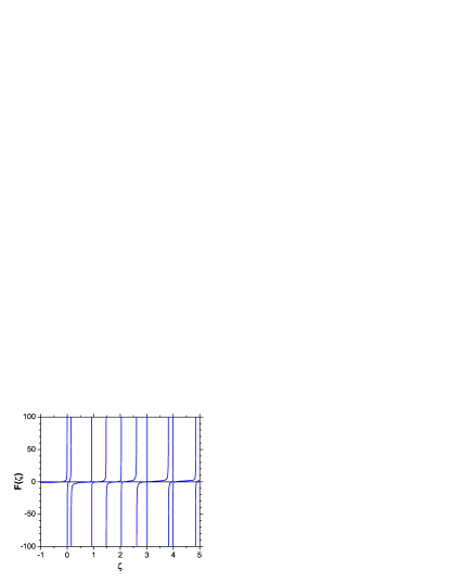
Figure 3: Plot of $F(\zeta)$ corresponding to the recurrence (80) of the Rabi model for $g=0.7$, $\Delta=0.4$, and $\omega=1$, i.e. the same parameters as for $G_{\pm}(\zeta)$ in Fig. 1 of Ref. Br , shows corresponding zeros at $\approx-0.217805$, $0.0629563$, $0.86095$, $1.1636$, $1.85076$, etc.

V.1 A comparison with Braak’s functions and integrability

In a recent letter Br , Braak claimed to have solved the Rabi model analytically (see also Viewpoint by Solano Sln ). He suggested Br that a regular spectrum of the Rabi model in the respective parity eigenspaces was given by the zeros of transcendental functions

$$G_{\pm}(\zeta)=\sum_{n=0}^{\infty}K_{n}(\zeta,\kappa)\left[1\mp\frac{\Delta}{\zeta-n}\right]\kappa^{n}.$$ (82)

Here the coefficients $K_{n}(\zeta,\kappa)$ were obtained recursively by solving the Poincaré difference equation (80) upwardly starting from the initial condition

$$K_{1}/K_{0}=f_{0}(\zeta)=2\kappa-\frac{1}{2\kappa}\left(\zeta-\frac{\Delta^{2}}{\zeta}\right).$$ (83)

In general that yields the coefficients $K_{n}$ as the dominant solution of the three-term recurrence (80) AMep .

Braak argued that between subsequent poles of the term in the square bracket in (82) at $\zeta=n$ and $\zeta=n+1$ the function $G_{\pm}(\zeta)$ takes on zero value:

• once - by implicitly presuming that at one of the poles $G_{\pm}(\zeta)$ goes to $+\infty$ and at the neighboring pole goes to $-\infty$, with a monotonic behavior from $+\infty$ to $-\infty$ between the poles;

• twice - implicitly presuming that $G_{\pm}(\zeta)$ goes to one of $\pm\infty$ at both subsequent poles of the term in the square bracket in (82), and in between the poles it has rather featureless behavior, e.g., similar to the cord hanging on two posts;

• none - occurs under the similar circumstances as described in the previous item, if the “cord is too short”, e.g., it does not stretch sufficiently up or down as to cross the abscissa.

Braak’s arguments regarding integrability of the Rabi model then rely heavily on the above properties. However, the above behavior can be merely regarded as an unproven hypothesis. There is no proof in Ref. Br that this is the only possible behavior. In this regard, Eqs. (80) and (81) show that $K_{n}(\zeta,\kappa)$ is a complicated sum of polynomial fractions with increasing polynomial degree in both the numerator and denominator. Any given $K_{n}(\zeta,\kappa)$ has its own zeros and poles structure for it comprises all singular terms $\Delta^{2}/(l-\zeta)$ between $l=0$ and $l=n-1$, including their mutual products. Additionally, in spite of the suggestive notation $K_{n}(\zeta)$ employed in Ref. Br , any $K_{n}(\zeta,\kappa)$ is a rational function of $\kappa$ comprising terms between $\kappa^{-n}$ and $\kappa^{n}$. Indeed, the $\Delta$-independent contribution to $K_{n}(\zeta,\kappa)$ is given by Eq. (74). Consequently, (i) the representation (82) hides additional poles in $\zeta$ and (ii) it cannot be excluded that between any two subsequent poles of the term in the square bracket in (82) the function $G_{\pm}(\zeta)$ would display much more complicated behavior than that assumed by Braak Br .

Analogous objections apply to the proposed functional form of $G_{\pm}(\zeta)$ in Eq. (6) of Ref. Br ,

$$G_{\pm}(\zeta)=G_{\pm}^{0}(\zeta)+\sum_{n=0}^{\infty}\frac{h_{n}^{\pm}}{\zeta-n},$$ (84)

where $G_{\pm}^{0}(\zeta)$ is entire in $\zeta$. Without any control over $G_{\pm}^{0}(\zeta)$ it is impossible to make any definite statement on the number of zeros of $G_{\pm}(\zeta)$ in any predetermined interval $\zeta\in(n,n+1)$. This should be contrasted with the Mittag-Leffler PFD (28) of our $F(x)$ function, which is much stronger result than Eq. (84) of Braak Br . There is no entire function contribution in our PFD (28). Additionally, Braak Br cannot say anything about the residues $h_{n}^{\pm}$, whereas the residues ${\cal M}_{k}$ in the Mittag-Leffler PFD (28) are all positive and given by Eq. (29).

V.2 Absence of degeneracies

In the case of a displaced harmonic oscillator, which is the special case of $\hat{H}_{R}$ in (1) for $\mu=0$, the recurrence (3) becomes (cf. Eq. (A.17) of Ref. Schw )

$$\phi_{n+1}+\frac{n-x}{(n+1)\kappa}\,\phi_{n}+\frac{1}{n+1}\,\phi_{n-1}=0.$$ (85)

The recurrence coefficients are nonsingular. Therefore, the uniqueness of the minimal solution $\{\phi_{n}\}_{n=0}^{\infty}$ of the recurrence (85) for any value of physical parameters Schw ; Gt ; AMep ; AMcm implies a unique entire function $\upvarphi(z)=\sum_{n=0}^{\infty}\phi_{n}z^{n}$ in the Bargmann space $\mathfrak{b}$. Consequently, the spectrum of the displaced harmonic oscillator when considered in $\mathfrak{b}$, i.e. (cf. Eq. (2.1) of Ref. Schw )

$$\hat{H}_{dho}=\omega\hat{a}^{\dagger}\hat{a}+\lambda(\hat{a}^{\dagger}+\hat{a}),$$ (86)

is necessarily nondegenerate with a unique eigenstate $\Phi(z)\equiv\upvarphi(z)\in\mathfrak{b}$ for any value of physical parameters. The spectrum becomes doubly-degenerate only if considered as the special case of $\hat{H}_{R}$ in Eq. (1) for $\mu=0$, i.e. when described by

$$\hat{H}_{dho}=\omega\mathds{1}\hat{a}^{\dagger}\hat{a}+\lambda\sigma_{3}(\hat{a}^{\dagger}+\hat{a})$$ (87)

in the product Hilbert space ${\cal B}=\mathfrak{b}\otimes\mathbb{C}^{2}$. In the latter case, the unique $\upvarphi(z)$ could be substituted into Eq. (13) to construct two different degenerate parity eigenstates $\Phi^{\pm}\in{\cal B}$.

As another example, consider the original parity unresolved recurrence for the Rabi model (80). The latter has the coefficients $a_{n}=-f_{n}(\zeta)/(n+1)$, where each $f_{n}(x)$ given by Eq. (81) has a simple pole at $\zeta=n\in\mathbb{N}$. At the singularities, the conditions which guarantee uniqueness of the minimal solution are violated. Therefore, degeneracies of the Rabi model could only occur at the baselines $\zeta=n\in\mathbb{N}$ (including $n=0$), where different parity solutions considered as a function of energy are allowed to intersect. Thereby the original result of Kus Ks has been rederived straightforwardly within our approach.

In the present case of parity resolved three-term recurrences for the Rabi model (14), the recurrence coefficients are regular and the recurrences (14) satisfy the conditions which guarantee uniqueness of the minimal solution for any value of physical parameters. Therefore, the spectrum in each parity eigenspace ${\cal B}_{\pm}$ is necessarily nondegenerate.

The nondegeneracy is not new result - it was initially obtained by Kus Ks within the framework of Frobenius’s analysis of regular singular points Frb . Yet it is both stimulating and inspiring that our approach based on OPS’s enabled us to prove the basic analytic property of the Rabi model independently, without any recourse to its earlier proof. The above examples show that the present approach is a powerful alternative to the Frobenius analysis Frb . Compared to the latter, it enables one to straightforwardly draw conclusions regarding the degeneracy or nondegeneracy of the spectrum simply by checking if the conditions which guarantee uniqueness of the minimal solution are satisfied (cf. the Poincaré theorem (Theorem 2.1 in Ref. Gt ), or the Perron and Kreuser generalizations the Poincaré theorem (Theorems 2.2 and 2.3(a) in Ref. Gt ).

Note in passing that the conventional recurrences (80) (for $\zeta\notin\mathbb{N}$) and (85) introduced by Schweber Schw represent the special case of Poincaré recurrences. The latter is characterized in that the respective coefficients $a_{n}$ and $b_{n}$ in (3) have finite limits $\bar{a}$ and $\bar{b}$ Schw ; Gt ; AMep ; AMcm . The recurrences (80) and (85) correspond to the choice of $\varsigma=0$ and $\upsilon=-1$ in Eq. (5), and yield $\tau=1$. They only differ in the value of $\bar{a}=-1/(2\kappa)$ in (80) and $\bar{a}=1/\kappa$ in (85), whereas $\bar{b}=0$ in both examples.

V.3 Algebraic solvability

The notion of quasi-exact solvability (QES) has been introduced to characterize the quantum models possessing a finite number of eigenvalues and corresponding eigenfunctions that can be determined algebraically TU ; Trb ; BD ; KUW . A typical quasi-exactly solvable Schrödinger operator can be expressed as a polynomial of degree at most two in the generators of the $sl(2,\mathbb{R})$ algebra Trb ; FGR ,

$$H=\sum_{k,m}q_{km}J_{k}^{n}J_{m}^{n}+\sum_{m}q_{m}J_{m}^{n}+q_{*},$$ (88)

where $q_{km}$, $q_{m}$, $q_{*}$ are some real constants,

$$J_{-}^{n}=\partial_{z},\leavevmode\nobreak\ \leavevmode\nobreak\ \leavevmode\nobreak\ \leavevmode\nobreak\ \leavevmode\nobreak\ J_{0}^{n}=z\partial_{z}-\frac{n}{2},\leavevmode\nobreak\ \leavevmode\nobreak\ \leavevmode\nobreak\ \leavevmode\nobreak\ \leavevmode\nobreak\ J_{+}^{n}=z^{2}\partial_{z}-nz,$$ (89)

$n$ is an integer, and

$$[J_{+}^{n},J_{-}^{n}]=2J_{0}^{n},\leavevmode\nobreak\ \leavevmode\nobreak\ \leavevmode\nobreak\ \leavevmode\nobreak\ \leavevmode\nobreak\ [J_{0}^{n},J_{\pm}^{n}]=\pm J_{\pm}^{n}.$$ (90)

The Rabi model KKT allows for such a representation in terms of the generators of $sl(2,\mathbb{R})$ algebra only for the energies corresponding to the eigenvalues of the displaced harmonic oscillator given by Eq. (75) (cf. Eq. (12) of Ref. KKT ), or equivalently for $\zeta=l\in\mathbb{N}$. The baselines $\upepsilon=l-\kappa^{2}$ have been identified in the preceding section as the only place where degenerate state could occur. This is indeed exemplified by the Juddian exact isolated analytic solutions Jd ; Ks ; KL . The latter correspond to the degenerate polynomial solutions of the Rabi model Ks . This shows that the very existence of the the parity degenerate Juddian exact isolated analytic solutions is a direct consequence of the quasi-exact solvability of the Rabi model KKT .

However, not any quasi-exactly solvable Schrödinger operator can be expressed in terms of the quadratic elements of an enveloping $sl(2,R)$ algebra KM . Therefore one might argue that an exact solvability for other energy values would still be possible. Nevertheless, the possibility of further polynomial solutions can be excluded by recent result by Zhang Zh . Indeed, let us consider the differential equation

$$\left[X(z)\frac{d^{2}}{dz^{2}}+Y(z)\frac{d}{dz}+Z(z)\right]\Psi(z)=0,$$ (91)

where $X(z)=\sum s_{k}z^{k}$, $Y(z)=\sum t_{k}z^{k}$, $Z(z)=\sum v_{k}z^{k}$ are polynomials of degree at most $4$, $3$, $2$, respectively. Zhang Zh found all polynomials $Z(z)$ such that Eq. (91) has polynomial solutions $\Psi(z)=\prod_{j=1}^{l}(z-z_{j})$ of degree $l$ with distinct roots $z_{j}$. Theorem 1.1 of Zhang Zh yields an algebraic conditions on each of the expansion coefficients $v_{k}$, $k=0,1,2$ of $Z(z)$ in terms of the expansion coefficients of $X(z)$, $Y(z)$, and of the roots $z_{j}$. In the case of the Schweber’s equation for the Rabi model [Eq. (3.23) of Ref. Schw ), and upon taking into account that Schweber’s $\kappa$ is twice of ours,

$$z(z-2\kappa)\frac{d^{2}\Psi(z)}{dz^{2}}$$

$$+\left[2(\kappa\zeta-\kappa)+(1-2\zeta+4\kappa^{2})z-2\kappa z^{2}\right]\frac{d\Psi(z)}{dz}$$

$$+\left[\zeta^{2}-\Delta^{2}-2\kappa\zeta(1-z)\right]\Psi(z)=0.$$ (92)

Because for the Rabi model Zhang’s $s_{4}=s_{3}=t_{3}=0$, Zhang’s condition (1.8) on $v_{2}$ reduces to $v_{2}=0$, and Zhang’s condition (1.9) on $v_{1}$ reduces to $v_{1}=-lt_{2}$, or, $\zeta=l$. The latter leads to Eq. (75), i.e., again to the Juddian exact isolated solutions Jd ; Ks ; KL . One arrives at the same conclusion if Zhang’s conditions Zh are applied to Eq. (5) of KKT , which is another variant of (92). Therefore, the Rabi model has no other polynomial solution than the Juddian exact isolated solutions. Any exact nondegenerate solution of the Rabi model is characterized by infinite set of nonzero expansion coefficients $\phi_{n}$, which for sufficiently large $n$ behave as $\phi_{n}\sim(-\kappa)^{n}/n!$ [cf. the Perron-Kreuser theorem (6) and the recurrence Eq. (14)]. It is not possible to have $\phi_{n}\equiv 0$ for $n>l$, where $l$ is some positive constant. Indeed, Eq. (14) reduces for $n=l+1$ to $\phi_{l}/(l+2)=0$, in contradiction to that $\phi_{l}\neq 0$. Only if two such solutions become degenerate, a linear combination of the solutions could result in a Juddian exact isolated analytic solution characterized in that $\phi_{n}\equiv 0$ for $n>l$.

V.4 Zeros of $\phi_{n}$ and the spectrum

In the case of the displaced harmonic oscillator, the solution of the recurrence for $\phi_{n}$ was given by Eq. (74). In general, rapid growths of the product $\prod_{k=0}^{n}(\zeta-k)$ in (74) essentially cancels out the $1/n!$ prefactor, leads to a finite radius of convergence of the series for $\upvarphi(z)$ in Eq. (4), and prevents $\upvarphi(z)$ from being an element of $\mathfrak{b}$. The points of the spectrum are characterized by a sudden collapse of the degree of $\phi_{n}$, which is in general polynomial of degree $n$ in energy, to a polynomial of merely the $(l-1)$th order for any $n\geq l$ at the $l$th spectral point (including $l=0$). Indeed, at the points of the spectrum $\zeta=\upepsilon+\kappa^{2}=j\in\mathbb{N}$ the sum over $j$ in Eq. (74) runs only between $j=0$ and $j=l-1$ for $n\geq l$. Otherwise the product on the right-hand side of Eq. (74) vanishes. The leading $(l-1)$th order in $\zeta$ is rapidly decreasing with increasing $n$ as

$$(-1)^{n+1-l}\frac{l\kappa^{n+2-2l}}{(n+1-l)!},$$ (93)

which implies $\upvarphi(z)\in\mathfrak{b}$ Schw . Thus the very same product terms $\prod_{k=0}^{j}(\zeta-k)$, which initially prevented $\upvarphi(z)$ from being an element of $\mathfrak{b}$, come later on to the rescue and ensure that $\upvarphi(z)\in\mathfrak{b}$ for the spectral points $\zeta\in\mathbb{N}$ (including $\zeta=0$).

It appears plausible that $\phi_{n}$’s can be expressed as a sum of such product terms involving the spectrum also in general case (e.g. for the Rabi model), and a point of the spectrum would then manifests itself by a sudden collapse of the degree, and magnitude, of $\phi_{n}$. The latter is necessary, because $\phi_{n}$ has to vanish in the limit $n\rightarrow\infty$ at the points of the spectrum in order to guarantee that $\upvarphi(z)\in\mathfrak{b}$. In the case of the displaced harmonic oscillator, the $\phi_{n}$’s are generated by the recurrence (48) as polynomials in $x$. The leading order of $\phi_{n}$ in $x$ is then provided by the polynomial term

$$\frac{1}{n!}\,\prod_{l=0}^{n-1}\left(x-\frac{l}{\kappa}\right).$$ (94)

However, starting from the recurrence (14), it is highly nontrivial to arrive at Eq. (74), and hence to identifying the spectrum, even in the exactly solvable case. Such a step from (14) to (74) is established neither here nor by Braak Br .

V.5 Compatibility

With increasing $n$, the PFD (60) defines a sequence of rational functions with simple real poles and positive residues. Kritikos ($\S 4$ of Ref. Krt ) showed that if the sequence of such rational functions

$$R_{n}(z)=\sum_{k=1}^{n}\frac{M_{nk}}{z-x_{nk}}$$ (95)

converges uniformly in a proximity of some point $z_{0}\in\mathbb{C}$, then the sequence converges everywhere in the complex plane with a possible exception of the real axis. The convergence is uniform in any bounded region of the complex plane with a nonzero distance from the real axis. The latter is obviously compatible with our main result.

In general one cannot always guarantee that, such as in Eq. (29), $M_{nk}\rightarrow{\cal M}_{k}=d\psi>0$ in the limit $n\rightarrow\infty$. Indeed, Theorem I in $\S 8$ of Grommer Gr merely ensures that for any $m>0$

$$\psi_{n}(x_{nk}-0) < \psi_{n+m}(x_{nk})<\psi_{n}(x_{nk})$$ (96)

$$= \psi_{n}(x_{n,k+1}-0)<\psi_{n+m}(x_{n,k+1}),\hskip 28.45274pt$$

where as usual $\psi_{n}(x-0)$ denotes the left-side limit of $\psi_{n}$ at $x$. On taking the limit $n\rightarrow\infty$ one cannot exclude that $\psi(\xi_{k})=\psi(\xi_{k+1})$ for some $k$, and hence $d\psi(\xi_{k+1})\equiv 0$. The above Grommer’s theorem appears to be related to the fact that, given the sharp inequality (27), $\xi_{k}^{(1)}$ could coincide with one of $\xi_{k}<\xi_{k+1}$. Because $\xi_{k}^{(1)}<\xi_{k+1}^{(1)}$, one can only exclude that two subsequent $\xi_{k}^{(1)}$ and $\xi_{k+1}^{(1)}$ coincide with a single $\xi_{k}$ or $\xi_{k+1}$. If $\xi_{k}^{(1)}=\xi_{k+1}$, then $d\psi(\xi_{k+1})=0$ in the Mittag-Leffler PFD (28). However, the latter can be prevented in the case of the Rabi model [cf. Eq. (70)].

V.6 Open problems

The dynamics and long-time evolution of the Rabi model is well understood only for rather weak couplings $\kappa=g/\omega\lesssim 10^{-2}$, where the Rabi model can be reliably approximated by the JC model JC ; SK . The latter was originally proposed as an exactly-solvable approximation to the Rabi model by applying the RWA and neglecting rapidly oscillating counterrotating terms JC ; SK . The JC model provides the basis for, from the Rabi model perspective somewhat misleadingly called, strong-coupling regime CRL ; KGK ; CC . The latter encompasses the cavity quantum electrodynamics and associated with it vacuum-field Rabi oscillations of atoms, molecules, and quantum-dots in a cavity KGK . Long-time behavior of various dynamical variables of the JC model can be described by analytic approximations ENS and the dynamics shows periodic spontaneous collapse and revival of coherence ENS ; Agr . With new experiments rapidly approaching the limit of the deep strong coupling regime characterized by $\kappa\gtrsim 1$ CRL , the question of major physical relevance is that of the dynamics of the Rabi model for $\kappa\gtrsim 0.1$ CRL ; FL ; WoK ; WVR . A great deal of insight into the dynamics of the Rabi model has been gained by Casanova et al. CRL in the limit $\omega_{0}/\omega\ll 1$ by means of an expansion in the small parameter $\omega_{0}/\omega$. Photon wave number packets were shown to propagate coherently along two independent parity chains of states and, like in the JC model ENS ; Agr , exhibited a collapse-revival pattern of the system population CRL . Nevertheless, still only very little is known about the dynamics in a very interesting physical region of $\omega_{0}/\omega\simeq 1$ CRL ; FL ; WoK ; WVR . The just established link between the Rabi model and the OPS’s could improve calculations of the eigenvalues and eigenfunctions, which are prerequisite for a reliable calculation of the dynamics of the Rabi model, and shed light on its long-time evolution for all values of the dimensionless coupling $\kappa$ CRL . Indeed, it can be shown that the number of calculated energy levels is almost two orders of magnitude higher AMtb than is possible to obtain by means of the alleged “analytical solution” of the Rabi model Br . The only numerical limitation in calculating zeros are over- and underflows in double precision. Typically, with increasing $n$ the respective recurrences yield first increasing and then decreasing $\phi_{n}$, $A_{n}$, and $B_{n}$. By using an elementary stepping algorithm this limits the total number of energy levels that can be determined to ca. 1350 levels per parity subspace, or to ca. 2700 levels for the Rabi model in total in double precision AMtb . It is conceivable that on using more sophisticated algorithm the number of calculable levels could be comparable to that obtained by numerical schemes involving diagonalization of tridiagonal matrices.

The nearest-neighbor energy level spacing distribution is customarily used to distinguish between integrable models and chaotic systems BT ; BGS ; ZR . Kus Ksc observed that neither Poissonian nor Wigner distributions can describe the level statistics for the Rabi model. Instead Kus Ksc found a nongeneric distribution of a “picket-fence” type. Our recent results suggest that the level statistics should resemble that of the zeros of suitable orthogonal polynomials AMtb . At the same time, the significantly larger number of computable energy levels within our approach enables one to perform a refined statistical analysis of the spectrum.

Carleman’s criterion states that the Hamburger moment problem associated with the positive-definite OPS (38) and (39) is determined (i.e., the Stieltjes weight function $\psi$ is unique), if the condition (67) is satisfied Chi . An alternative sufficient condition for the determinacy of the classical Hamburger moment problem is that the moments (57) of the positive moment functional ${\cal L}$ have to satisfy (cf. Eq. (3) of Ref. Hb ; $\S 5$ of Ref. Hb0 )

$$|\mu_{n}|\leq\frac{\theta}{\Lambda^{n}}\,n!,$$ (97)

where $\theta$ and $\Lambda$ are two real positive constants. Hamburger’s condition (97) is also sufficient condition for the uniform convergence of the associated infinite continued fraction in any closed domain $\Omega$ of the complex plane which does not contain any part of the real axis Hb . The sequence of convergents in Eqs. (19) and (60) then converges uniformly to the infinite continued fraction in Eq. (9), which ensures the convergence of the latter Hb (see also pp. 214-215 of Ref. Hb0 ). This raises the question regarding a mutual relation between the respective asymptotic behaviors of the $\lambda_{n}$’s and $\mu_{n}$’s. In the special case of $c_{n}\equiv 0$ in Eq. (38) for all $n\in\mathbb{N}$, Bender and Milton BM showed that $\lambda_{n}\sim n$ implies $\mu_{n}\sim n!$ and vice versa. It would be interesting to prove rigorously if such a relation holds also in more general case of $c_{n}\neq 0$, such as for the Rabi model.

Last but not the least, an interesting question is if the ideas presented here could also be extended to systems characterized by a three-term difference equation (3) with periodic coefficients, like in the Hofstadter problem of Bloch electrons in rational magnetic fields Hf .

VI Conclusions

On applying the theory of orthogonal polynomials, the eigenvalue equation and eigenfunctions of the quasi-exactly solvable Rabi model was shown to be determined in terms of three systems of monic orthogonal polynomials. The formal Schweber quantization criterion for an energy variable $x$, originally expressed in terms of infinite continued fractions, was shown to be equivalent to a meromorphic function $F(x)$ in the complex plane $\mathbb{C}$. $F(x)$ can be expressed by the partial fraction decomposition (28) with real simple poles and positive residues ${\cal M}_{k}$ defined by (29). Thereby the calculation of spectrum corresponding to the zeros of $F(x)$ was greatly facilitated. One obtains at once that (i) $F(x)$ monotonically decreases from $+\infty$ to $-\infty$ between any two of its subsequent poles $\xi_{k}$ and $\xi_{k+1}$, (ii) there is exactly one zero of $F(x)$ for $x\in(\xi_{k},\xi_{k+1})$, and (iii) the spectrum corresponding to the zeros of $F(x)$ does not have any accumulation point. Additionally, one can provide much simpler proof of that the spectrum in each parity eigenspace ${\cal B}_{\pm}$ is necessarily nondegenerate. Recent claims regarding solvability and integrability of the Rabi model Br ; Sln were critically examined. Compatibility of our results with some other results of the theory of infinite continued fractions and complex analysis was explicitly demonstrated.

VII Acknowledgment

I like to thank anonymous referees for valuable comments. Continuous support of MAKM is largely acknowledged.

Appendix A Technical remarks

Assuming that the power series $\sum_{n=0}^{\infty}\mu_{n}/z^{n}$ has a nonzero radius of convergence $|z|>R>0$, i.e., much weaker condition than Hamburger’s condition (97), Grommer arrived from an integral representation (cf. Eq. (63) of Ref. Gr )

$$f(z)=\int_{-R}^{R}\frac{d\psi(x)}{z-x}$$ (98)

to the Mittag-Leffler PFD (cf. Eq. (66) of Ref. Gr )

$$f(z)=\sum_{j=1}^{\infty}\frac{{\cal M}_{j}}{z-\xi_{j}}\cdot$$ (99)

Essential to his arguments was that $f(z)$ remained finite and different from zero for any nonreal $z\in\mathbb{C}$. However, in virtue of

$$\int_{-\infty}^{\infty}\frac{dx}{(u-x)^{2}+q^{2}}=\frac{\pi}{q}<\infty,$$ (100)

the very same is also true if the integration range in Eq. (98) were, such as in our case, extended to infinity.

By making use of the Nevanlinna theorem N (later rediscovered by Sokal So in his improvement of Watson’s theorem on Borel summability; for an extension of the Nevanlinna-Sokal theorem to differently shaped region see Ref. AMcmp ), which was not known to Hamburger at the time he wrote his Hb , one can immediately amend Hamburger theorem under his item 4 on pp. 33-34 of Hb . One can prove that Hamburger’s function $f(z)$ is asymptotically represented by the power series $S(z)$ not merely in an angular domain $\varepsilon\leq\arg z\leq\pi-\varepsilon$, where $\varepsilon$ an arbitrary small positive infinitesimal, but rather in a disc tangent to the real axis.

The zeros of $P_{n}(x)$ can be associated with eigenvalues of Jacobi matrices. The latter are derived from the coefficients of the recurrence (38) upon writing each $\lambda_{n}>0$ as a product of two complex conjugate numbers $\lambda_{n}=z_{n}z_{n}^{*}$, and assembling them into the Hermitian matrix

$$M_{n}=\left[\begin{array}[]{ccccccc}c_{1}&z_{2}&0&\ldots&0&0&0\\ z_{2}^{*}&c_{2}&z_{3}&\ldots&0&0&0\\ 0&z_{3}^{*}&c_{3}&\ldots&0&0&0\\ \cdot&\cdot&\cdot&\ldots&\cdot&\cdot&\cdot\\ 0&0&0&\ldots&z_{n-1}^{*}&c_{n-1}&z_{n}\\ 0&0&0&\ldots&0&z_{n}^{*}&c_{n}\end{array}\right].$$ (101)

Then the eigenvalues of $M_{n}$ are the zeros of $P_{n}(x)$. (Ex. I-5.7 on p. 30 of Ref. Chi ).

Using the results of Hamburger Hb , one can prove that

$$w_{n}(t)=\sum_{k=1}^{n}M_{nk}\,e^{x_{nk}t}$$ (102)

converges uniformly toward

$$W(t)=\sum_{n=0}^{\infty}\frac{\mu_{n}}{n!}\,t^{n}$$ (103)

within any vertical stripe $|t|\leq R-\delta$, where $R>0$ is a nonzero radius of convergence of the series for $W(t)$ and $\delta$ is some infinitesimally small number. The continued fraction in Eqs. (9) and (32) converges then uniformly to the Borel transform

$$F(z)=a_{0}+\int_{0}^{-i\infty}W(t)\,e^{-tz}\,dt$$ (104)

in any closed domain of the complex plane with Im $z\geq\delta>0$ (cf. $\S 3$ of Ref. Hb ).

References

- (1) I. I. Rabi, Phys. Rev. 49, 324 (1936); Phys. Rev. 51, 652 (1937).
- (2) S. Schweber, Ann. Phys. (N.Y.) 41, 205 (1967).
- (3) D. Braak, Phys. Rev. Lett. 107, 100401 (2011).
- (4) L. Yu, S. Zhu, Q. Liang, G. Chen, and S. Jia, Phys. Rev. A 86, 015803 (2012).
- (5) E. T. Jaynes and F. W. Cummings, Proc. IEEE 51, 89 (1963).
- (6) B. W. Shore and P. L. Knight J. Mod. Opt. 40, 1195 (1993).
- (7) G. Khitrova, H. M. Gibbs, M. Kira, S. W. Koch, and A. Scherer, Nat. Phys. 2, 81 (2006).
- (8) J. Bourassa, J. M. Gambetta, A. A. Abdumalikov, Jr., O. Astafiev, Y. Nakamura, and A. Blais, Phys. Rev. A 80, 032109 (2009).
- (9) P. Forn-Díaz, J. Lisenfeld, D. Marcos, J. J. García-Ripoll, E. Solano, C. J. P. M. Harmans, and J. E. Mooij, Phys. Rev. Lett. 105, 237001 (2010).
- (10) T. Niemczyk et al, Nature Phys. 6, 772 (2010).
- (11) C. Ciuti and I. Carusotto, Phys. Rev. A 74, 033811 (2006).
- (12) J. Casanova, G. Romero, I. Lizuain, J. J. García-Ripoll, and E. Solano, Phys. Rev. Lett. 105, 263603 (2010).
- (13) E. Solano, Physics 4, 68 (2011).
- (14) A. V. Turbiner and A. G. Ushveridze, Phys. Lett. A 126, 181 (1987).
- (15) A. V. Turbiner, Commun. Math. Phys. 118, 467 (1988).
- (16) C. M. Bender and G. V. Dunne, J. Math. Phys. 37, 6 (1996).
- (17) A. Krajewska, A. Ushveridze, Z. Walczak, hep-th/9601088.
- (18) R. Koc, M. Koca, and H. Tütüncüler, J. Phys. A: Math. Gen. 35, 9425 (2002).
- (19) B. R. Judd, J. Phys. C: Solid State Phys. 12, 1685 (1979).
- (20) M. Kus, J. Math. Phys. 26, 2792 (1985).
- (21) M. Kus and M. Lewenstein, J. Phys. A: Math. Gen. 19, 305 (1986).
- (22) I. D. Feranchuk, L. I. Komarov, and A. P. Ulyanenkov, J. Phys. A: Math. Gen. 29, 4035 (1996).
- (23) E. K. Irish, Phys. Rev. Lett. 99, 173601 (2007).
- (24) A. Moroz, Europhys. Lett. 100, 60010 (2012).
- (25) V. Bargmann, Comm. Pure Appl. Math. 14, 187 (1961).
- (26) W. Gautschi, SIAM Review 9, 24 (1967).
- (27) A. Moroz, arXiv:1205.3139.
- (28) R. L. Fulton and M. Gouterman, J. Chem. Phys. 35, 1059 (1961).
-
(29)
The source code can be freely downloaded from
http://www.wave-scattering.com/rabi.html. -
(30)
http://en.wikipedia.org/wiki/Frobenius_method - (31) T. S. Chihara, An Introduction to Orthogonal Polynomials (Gordon and Breach, New York, 1978).
-
(32)
The necessary and sufficient condition for a family of
polynomials (with
degree ) to form an orthogonal polynomial system
is that ’s satisfy a three-term recursion relation