MHD modeling of solar system processes on geodesic grids

Abstract

This report describes a new magnetohydrodynamic numerical model based on a hexagonal spherical geodesic grid. The model is designed to simulate astrophysical flows of partially ionized plasmas around a central compact object, such as a star or a planet with a magnetic field. The geodesic grid, produced by a recursive subdivision of a base platonic solid (an icosahedron), is free from control volume singularities inherent in spherical polar grids. Multiple populations of plasma and neutral particles, coupled via charge-exchange interactions, can be simulated simultaneously with this model. Our numerical scheme uses piecewise linear reconstruction on a surface of a sphere in a local two-dimensional “Cartesian” frame. The code employs HLL-type approximate Riemann solvers and includes facilities to control the divergence of magnetic field and maintain pressure positivity. Several test solutions are discussed, including a problem of an interaction between the solar wind and the local interstellar medium, and a simulation of Earth’s magnetosphere.

1 Introduction

Many astrophysical plasma processes occur is regions of space surrounding a central compact object such as a star or a planet. Examples include stellar winds, planetary magnetospheres, supernova blast waves, and mass accretion onto compact objects. In all these environments the central body (a star or a planet) is typically much smaller than the characteristic scales of the plasma flows. In solving this class of problem on a computer, radial grids are commonly used because resolution can be readily increased near the origin. The simplest and the most commonly used is the standard spherical polar ($r$, $\theta$, $\varphi$) grid (e.g., Washimi & Tanaka, 1996; Pogorelov & Matsuda, 1998; Ratkiewicz et al., 1998). This grid has a singularity on the $z$ axis, where the control volume $\Delta V=r^{2}\Delta r\sin\theta\Delta\theta\Delta\varphi$, $\Delta r$, $\Delta\theta$ and $\Delta\varphi$ being the grid cell dimensions in the radial, latitudinal, and azimuthal directions, respectively, vanishes as $\sin\theta\to 0$. For explicit methods, this requires a small global time step to satisfy the Courant stability condition for a system of hyperbolic conservation laws for the entire grid (implicit or semi-implicit methods (e.g., Tóth et al., 1998) don’t suffer from this limitation).

Spherical grids are also used in simulating the transport of energetic charged particle, such as galactic cosmic rays, in turbulent astrophysical flows (Florinski & Pogorelov, 2009). Transport models based on stochastic trajectory (Monte-Carlo) methods also suffer from the singularity on the polar axis. For example, in modeling cosmic-ray transport in the heliosphere it is common to align the $z$ axis with the solar rotation axis. Because energetic particle transport (diffusion and drift) is very rapid at high latitudes due to a weaker magnetic field, a model must take vanishingly small time steps when a particle ventures close to the polar axis, which results in an inferior overall model efficiency.

Time step requirements can be relaxed substantially by employing a grid that has a (nearly) uniform solid angle coverage. Examples include triangle, hexagon, or diamond based geodesic grids (Du et al., 2003; Yeh, 2007; Upadhyaya et al., 2010), obtained by a recursive division of a base platonic solid, and cubed sphere grids (Ronchi et al., 1996; Putman & Lin, 2007). This paper introduces a framework for finite volume methods of solution of hyperbolic conservation laws in three dimensions, such as gas-dynamic or MHD systems, using spherical geodesic grids composed of hexagonal prism elements. Results are illustrated on a three-dimensional simulation of solar rotation and formation of corotating interaction regions (CIRs), an interaction between the solar wind and the surrounding local interstellar medium or LISM, and a simulation of Earth’s magnetosphere. The new framework can be employed to model a broad range of large-scale 3D astrophysical plasma flows around a compact object where high computational efficiency is a priority.

2 Grid structure

Our three-dimensional grid consist of a 2D geodesic unstructured grid on a sphere combined with a concentric nonuniform radial stepping with smaller cells near the origin. The 2D surface grid is a Voronoi tesselation of a sphere produced from a dual triangular (Delaunay) tesselation. The latter is generated by a recursive subdivision of an icosahedron. We use the geodesic grid generator software developed by the ICON project (http://icon.enes.org) for use in atmospheric circulation modeling. An optimization algorithm (Heikes & Randall, 1995), included in their code, produces a mesh with a difference in spherical surface areas between the largest and the smallest cells of less than 10%.

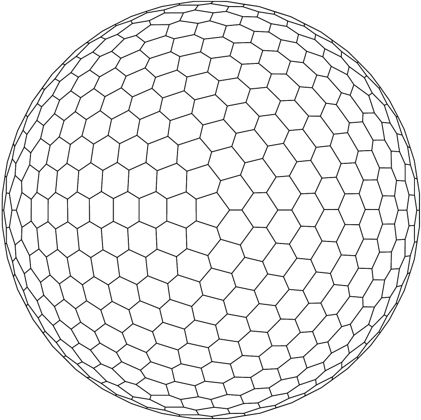
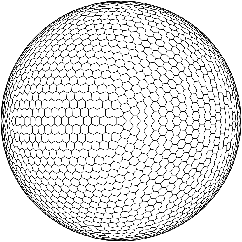
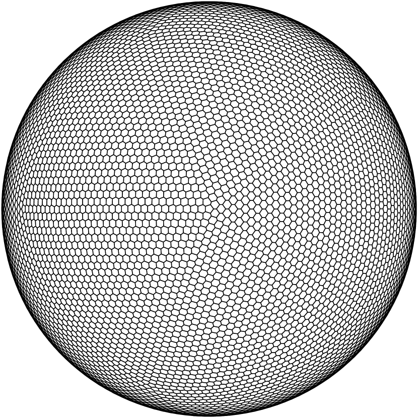
Figure 1: From left to right: level 3, 4, and 5 geodesic Voronoi grids produced by a recursive division of the base icosahedron.

The number of vertices (V), edges (E) and faces (F) on a grid produced by $l$th division is given by

$$N_{\mathrm{V}}=20\cdot 2^{2l},\quad N_{\mathrm{E}}=30\cdot 2^{2l},\quad N_{\mathrm{F}}=10\cdot 2^{2l}+2.$$ (1)

In this notation a level 0 grid is dual to the original icosahedron projected onto a unit sphere. The base shape of a control volume in a finite volume method is a spherical hexagonal prism with the exception of 12 pentagonal prisms located at the vertices of the original icosahedron. Level 3, 4, and 5 hexagonal geodesic grids are shown in Figure 1.

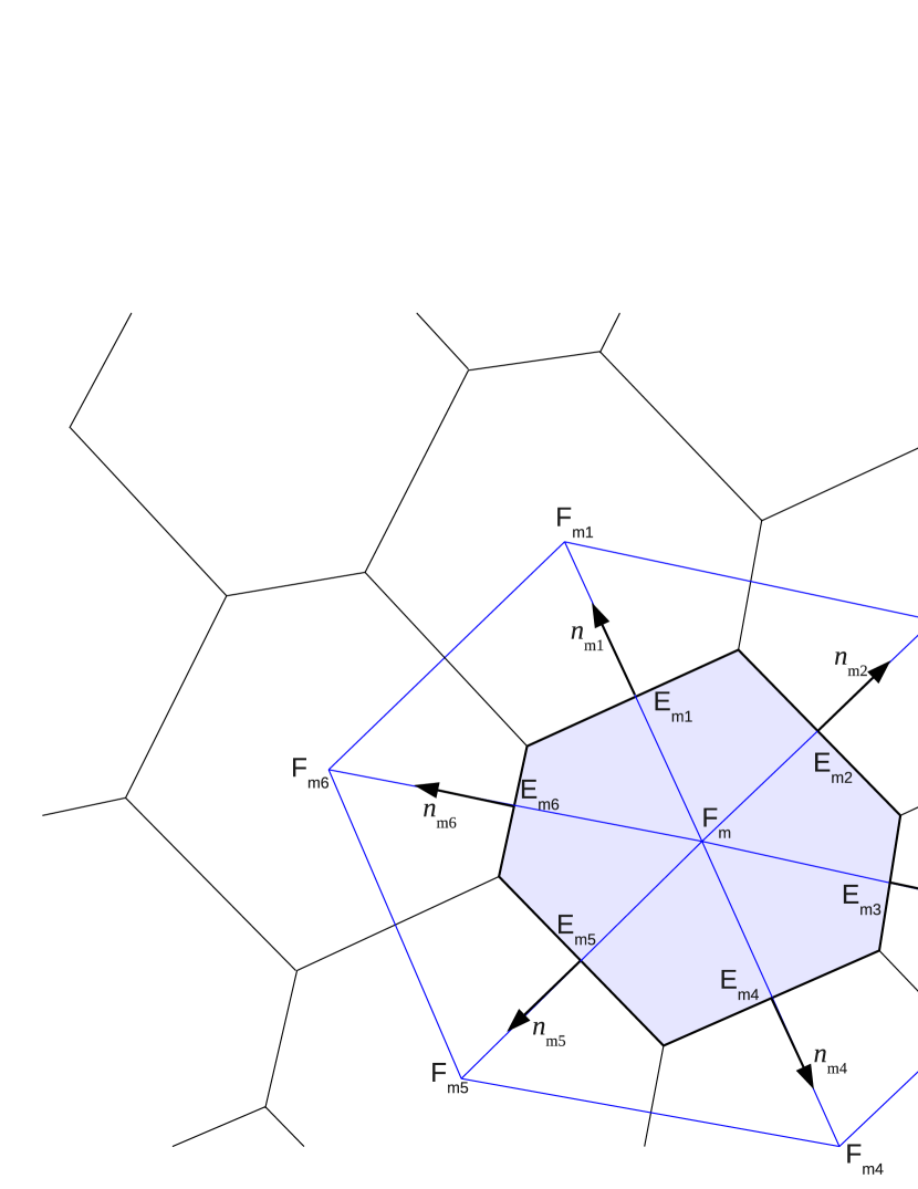
Figure 2: A close up view of the geodesic grid illustrating the relationships between a face $\mathrm{F}_{m}$ and its neighboring faces $\mathrm{F}_{m1}..\mathrm{F}_{m6}$. Unit vectors normal to the edges of the Voronoi face $\hat{\mathbf{n}}_{m1}..\hat{\mathbf{n}}_{m6}$ are shown. A fragment of the Delaunay grid is drawn with blue lines.

A more detailed view of the Voronoi grid structure is given in Figure 2. A hexagonal face $\mathrm{F}_{m}$ (shaded) is shown surrounded by six adjacent faces $\mathrm{F}_{m1}..\mathrm{F}_{m6}$. The face centers of the dual triangle-based Delaunay grid (blue lines) are located at the Voronoi vertices (V); likewise, the former’s vertices are at the Voronoi grid’s face centers (F). The edges of the Voronoi and Delaunay grids on a sphere are mutually orthogonal and intersect at their midpoints. To achieve acceptable resolution in typical astrophysical flow modeling problems level 5 or higher geodesic grids should be used. Most of our simulations use level 6 mesh containing 40,962 Voronoi polygons. We emphasize that these 40,962 hexagons are distributed evenly over the surface of each spherical layer of cells. This gives us a resolution of about $3\times 10^{-4}$ steradians in solid angle which corresponds to an angular resolution of one degree. By condensing the mesh in the radial direction, one can achieve a further degree of refinement as required by the problem.

We introduce a set of unit vectors normal to the edges of the Voronoi grid $\hat{\mathbf{n}}_{mn}$, where the index $m$ refers to the $m$th face and $n=[1,6]$ is the number of the edge counted in a counter-clockwise direction. The unit vectors are tangential to the surface of the sphere. The corresponding edge lengths, measured along great circles, are designated $L_{mn}$. The outward radial unit vector at the cell center is $\hat{\mathbf{r}}_{m}$. We also designate the area of the face on the unit sphere as $A_{m}$. In this notation the control volume is equal to

$$\Delta V_{im}=A_{m}r_{i}^{2}\Delta r_{i},$$ (2)

where $i$ is the index on the radial axis. The areas $A_{m}$ are calculated by dividing each hexagonal face into six (five for pentagons) spherical triangles and adding up their areas using standard expressions from spherical trigonometry. Having defined our cell dimensions is this way we can proceed to integrate a system of conservation laws inside a control volume.

It is worth pointing out that a similar geodesic-mesh-based model was developed by Nakamizo et al. (2009) Their mesh was generated from a dodecahedron by first dividing each face into five triangles followed by a recursive subdivision of each triangle into four smaller triangles. The resulting unstructured grid topology is similar (but not identical) to our dual Delaunay grid. Interestingly, in the model of Nakamizo et al. (2009) computations are also performed on a hexagonal grid, generated by connecting the centroids of the Delaunay triangles.

3 MHD conservation laws

For the heliospheric and magnetospheric problems (§6) we solve a modified set of MHD equations, written in terms of conservative variables $\mathbf{U}$ and fluxes $\mathbf{F}$ as

$$\frac{\partial\mathbf{U}}{\partial t}+\nabla\cdot\mathbf{F}=\mathbf{Q},$$ (3)

where

$$\mathbf{U}=\left(\begin{array}[]{c}\rho\\ \rho\mathbf{u}\\ e\\ \mathbf{B}\end{array}\right),\quad\mathbf{F}=\left(\begin{array}[]{c}\rho\mathbf{u}\\ \rho\mathbf{u}\mathbf{u}+p\mathbf{I}-\mathbf{B}\mathbf{B}/(4\pi)\\ (e+p)\mathbf{u}-\mathbf{B}(\mathbf{u}\cdot\mathbf{B})/(4\pi)\\ \mathbf{u}\mathbf{B}-\mathbf{B}\mathbf{u}\end{array}\right)$$ (4)

in CGS units. Here $\rho$ is density, $\mathbf{u}$ is velocity, $\mathbf{B}$ is magnetic field, $\mathbf{I}$ is a unit dyadic, $p=p_{\mathrm{g}}+B^{2}/(8\pi)$ is the total pressure, $p_{\mathrm{g}}$ being the gas kinetic pressure, and the energy density $e$ is given by

$$e=\frac{\rho u^{2}}{2}+\frac{p_{\mathrm{g}}}{\gamma-1}+\frac{B^{2}}{8\pi}.$$ (5)

We employ two alternative models to control the divergence of magnetic field. The first is the numerical scheme proposed by Powell et al. (1999), where numerical magnetic field divergence is advected out of the simulation domain with the flow velocity. This scheme modifies the system of conservation laws with a hyperbolic source term

$$\mathbf{Q}=-\nabla\cdot\mathbf{B}\left(\begin{array}[]{c}0\\ \mathbf{B}/(4\pi)\\ \mathbf{u}\cdot\mathbf{B}/(4\pi)\\ \mathbf{u}\end{array}\right).$$ (6)

The second scheme employs a generalized Lagrange multiplier (GLM) $\psi$ for a mixed hyperbolic-parabolic correction (Dedner et al., 2002). The system (4) is extended with an additional transport equation for $\psi$

$$\frac{\partial\psi}{\partial t}+\nabla\cdot(c_{h}^{2}\mathbf{B})=-\frac{c_{h}^{2}}{c_{p}^{2}}\psi,$$ (7)

where $c_{h}$ is a constant, isotropic advection speed, taken to be somewhat faster than the fastest wave speed in the problem, and $c_{p}$ is related to the rate of decay of $\psi$. Dedner et al. (2002) proposed two methods to fix the value of $c_{p}$: (a) by fixing the time rate of decay of the GLM variable $r_{d}=\exp(-\Delta tc_{h}^{2}/c_{p}^{2})$, where $\Delta t$ is the time step, and (b) by fixing the characteristic length over which the decay occurs, given by $l_{d}=c_{p}^{2}/c_{h}$. Both methods are available in our code. In the GLM scheme the conservation law for magnetic field (Faraday’s law) is modified to read

$$\frac{\partial\mathbf{B}}{\partial t}+\nabla\cdot(\mathbf{u}\mathbf{B}-\mathbf{B}\mathbf{u}+\psi\mathbf{I})=0.$$ (8)

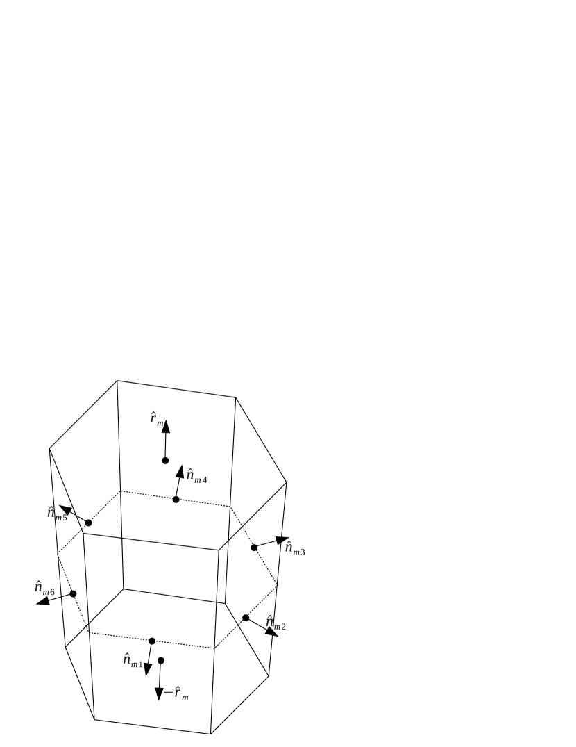
Figure 3: A prismatic control volume showing the unit vectors normal to the interfaces.

The system (3) is integrated over a control volume $\Delta V_{im}$ shown in Figure 3 to obtain the finite volume method

$$\Delta V_{im}\frac{\Delta\mathbf{U}_{im}}{\Delta t}=-A_{m}\left(r_{i+1/2}^{2}\mathbf{F}_{i+1/2,m}-r_{i-1/2}^{2}\mathbf{F}_{i-1/2,m}\right)\cdot\hat{\mathbf{r}}_{m}$$

$$-r_{i}\Delta r_{i}\sum_{n=1}^{6}L_{mn}\mathbf{F}_{i(mn)}\cdot\hat{\mathbf{n}}_{mn}+\Delta V_{im}\mathbf{Q}_{im}.$$ (9)

Here $\mathbf{F}_{i(mn)}$ is the flux at the center of the edge shared by the $m$th cell and its $n$th neighbor (where $n=[1,6]$). Note that the source term $\mathbf{Q}$ does not involve the right hand side of Eq. (7). The parabolic correction is applied by multiplying the value of $\psi$ obtained from the finite volume scheme (9) by the decay factor,

$$\psi\to\psi\times\left\{\begin{array}[]{ll}r_{d},&\mathrm{method\;(a)},\\ e^{-\Delta tc_{h}/l_{d}},&\mathrm{method\;(b)}.\end{array}\right.$$ (10)

In our simulations we typically use $0.9<r_{d}<1$ and $l_{d}$ equal to several times the smallest linear grid size.

The divergence of the magnetic field is obtained from Gauss’s theorem in the same way as $\nabla\cdot\mathbf{F}$ is calculated in Eq. (9). More generally, the divergence and curl operators acting on an arbitrary vector $\mathbf{v}$ may be written as

$$\nabla\cdot\mathbf{v}=\frac{\hat{\mathbf{r}}_{m}\cdot(r_{i+1/2}^{2}\mathbf{v}_{i+1/2,m}-r_{i-1/2}^{2}\mathbf{v}_{i-1/2,m})}{r_{i}^{2}\Delta r_{i}}+\sum_{n=1}^{6}\frac{L_{mn}\hat{\mathbf{n}}_{mn}\cdot\mathbf{v}_{i(mn)}}{r_{i}A_{m}},$$ (11)

$$\nabla\times\mathbf{v}=\frac{\hat{\mathbf{r}}_{m}\times(r_{i+1/2}^{2}\mathbf{v}_{i+1/2,m}-r_{i-1/2}^{2}\mathbf{v}_{i-1/2,m})}{r_{i}^{2}\Delta r_{i}}+\sum_{n=1}^{6}\frac{L_{mn}\hat{\mathbf{n}}_{mn}\times\mathbf{v}_{i(mn)}}{r_{i}A_{m}}.$$ (12)

An evaluation of a curl is necessary when modeling energetic charged particle transport, where the particle’s drift velocity is proportional to $\nabla\times(\mathbf{B}/B^{2})$. The values of primitive variables at face centers $\mathbf{v}_{i\pm 1/2}$ and $\mathbf{v}_{i(mn)}$ may be approximated as arithmetic averages of the values in the two cells separated by the face. A more accurate approach, adopted here, is to use interface resolved states obtained from a solution to the corresponding Riemann problem (see §5).

The finite volume system of conservation laws is integrated with a second order unsplit TVD-like method (see below). Right and left interface values are calculated in the usual way using some appropriate linear reconstruction to achieve second-order spatial accuracy. Fluxes are calculated from a solution to a one-dimensional (projected) Riemann problem at each cell interface. Finally, time is advanced using either a first order (Euler) or, more commonly, a second order (Runge-Kutta) scheme, depending on the nature of the problem.

4 Reconstruction

To achieve second order spatial accuracy we employ limited piecewise linear reconstruction on primitive variables $\mathbf{V}=(\rho,\mathbf{u},p_{\mathrm{g}},\mathbf{B},\psi)^{T}$. In the radial direction the simplest and the most robust limiter available is the MinMod, with slopes $\mathbf{S}_{im}$ given by

$$\mathbf{S}^{\mathrm{MM}}_{im}=\mathrm{minmod}(\mathbf{S}^{-}_{im},\mathbf{S}^{+}_{im}),$$ (13)

where the left and the right slopes on an asymmetric stencil are, respectively

$$\mathbf{S}^{-}_{im}=2\frac{\mathbf{V}_{im}-\mathbf{V}_{i-1,m}}{\Delta r_{i-1}+\Delta r_{i}},\quad\mathbf{S}^{+}_{im}=2\frac{\mathbf{V}_{i+1,m}-\mathbf{V}_{im}}{\Delta r_{i}+\Delta r_{i+1}}.$$ (14)

Also available is the more compressive monotonized central (MC) limiter (van Leer, 1977) with

$$\mathbf{S}^{\mathrm{MC}}_{im}=\mathrm{minmod}\left[2\mathbf{S}^{-}_{im},2\mathbf{S}^{+}_{im},\frac{(\Delta r_{i}+\Delta r_{i+1})\mathbf{S}^{-}_{im}+(\Delta r_{i-1}+\Delta r_{i})\mathbf{S}^{+}_{im}}{\Delta r_{i-1}+2\Delta r_{i}+\Delta r_{i+1}}\right].$$ (15)

The third option is the weighted essentially non-oscillatory (WENO) limiter

$$\mathbf{S}^{\mathrm{WENO}}_{im}=\bar{\mathbf{w}}^{-}_{im}\mathbf{S}^{-}_{im}+\bar{\mathbf{w}}^{+}_{im}\mathbf{S}^{+}_{im},$$ (16)

where the WENO weights $\bar{\mathbf{w}}$ are given by

$$\bar{\mathbf{w}}^{-}_{im}=\frac{({\mathbf{S}^{-}_{im}}^{2}+\epsilon)^{-p}}{({\mathbf{S}^{-}_{im}}^{2}+\epsilon)^{-p}+({\mathbf{S}^{+}_{im}}^{2}+\epsilon)^{-p}},\quad\bar{\mathbf{w}}^{+}_{im}=\frac{({\mathbf{S}^{+}_{im}}^{2}+\epsilon)^{-p}}{({\mathbf{S}^{-}_{im}}^{2}+\epsilon)^{-p}+({\mathbf{S}^{+}_{im}}^{2}+\epsilon)^{-p}},$$ (17)

where $p$ is an integer constant here taken to be 2, and $\epsilon$ is a small number, which we took to be $10^{-12}$ in our simulations. The $(\mathbf{S}^{+}_{im})^{2p}$ and $(\mathbf{S}^{-}_{im})^{2p}$ terms are traditionally referred to as smoothness measures in WENO methodology.

For two-dimensional reconstruction on the surface of a sphere the code can use either a minimum angle plane (MAPR) method (Christov & Popov, 2008) or a 2D version of the weighted essentially non-oscillatory (WENO) scheme (Friedrich, 1998). Common to both schemes, a local two-dimensional coordinate system ($\xi$,$\eta$) is introduced on the sphere, with its origin at the face center F_m. The coordinates of the six adjacent cell centers ($\xi_{mn}$, $\eta_{mn}$) are then calculated in this frame. These coordinates are measured along two arbitrary great circles intersecting at right angles at the position of the central face F_m. The procedure is illustrated in Figure 4. The angle $A$ and the great circle distance between the face centers $c$ are effectively polar coordinates on the surface of a sphere. The local coordinates of F_mn are calculated as

$$\xi_{mn}=c\cos A,\quad\eta_{mn}=c\sin A.$$ (18)

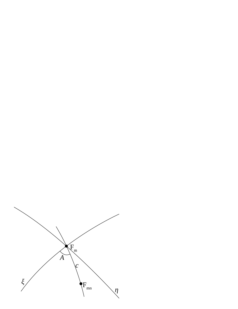
Figure 4: Calculation of adjacent cell center (F_mn) coordinates in a local coordinate frame associated with a face F_m. Every line shown is a segment of a great circle.

Next, the six two-dimensional slopes $\mathbf{S}^{\xi}$, $\mathbf{S}^{\eta}$ are calculated from the triangles with vertices located at the cell centers F_m, F_mn, F_m,n+1 (shown in blue in Figure 2) as

$$\mathbf{S}^{\xi}_{imn}=\frac{\eta_{mn}(\mathbf{V}_{im,n+1}-\mathbf{V}_{im})-\eta_{m,n+1}(\mathbf{V}_{imn}-\mathbf{V}_{im})}{\eta_{mn}\xi_{m,n+1}-\xi_{mn}\eta_{m,n+1}},$$ (19)

$$\mathbf{S}^{\eta}_{imn}=-\frac{\xi_{mn}(\mathbf{V}_{im,n+1}-\mathbf{V}_{im})-\xi_{m,n+1}(\mathbf{V}_{imn}-\mathbf{V}_{im})}{\eta_{mn}\xi_{m,n+1}-\xi_{mn}\eta_{m,n+1}}.$$ (20)

In the MAPR method we evaluated the average slopes as

$$\bar{\mathbf{S}}_{imn}=\sqrt{{\mathbf{S}^{\xi}_{imn}}^{2}+{\mathbf{S}^{\eta}_{imn}}^{2}}.$$ (21)

The reconstructed slopes $\mathbf{S}^{\mathrm{MAPR}\,\xi,\eta}_{im}$ are those given by Eqs. (19) and (20) for which the average slope (20) is the smallest. Thus the method is a two-dimensional equivalent of the MinMod limiter. In the WENO method the reconstructed slopes are weighted arithmetic averages of all six slopes, namely

$$\mathbf{S}^{\mathrm{WENO}\,\xi,\eta}_{im}=\sum_{n=1}^{6}\bar{\mathbf{w}}_{imn}\mathbf{S}^{\xi,\eta}_{imn}.$$ (22)

The weights $\bar{\mathbf{w}}_{imn}$ of each slope are calculated as

$$\bar{\mathbf{w}}_{imn}=\frac{\mathbf{w}_{imn}}{\sum_{n}\mathbf{w}_{imn}},$$ (23)

where

$$\mathbf{w}_{imn}=\left({\mathbf{S}^{\xi}_{imn}}^{2}+{\mathbf{S}^{\eta}_{imn}}^{2}+\epsilon\right)^{-p},$$ (24)

where we again use $p=2$ and $\epsilon=10^{-12}$. Because edge centers lie midway between the corresponding two face centers F_m and F_mn on the Voronoi grid, the reconstructed values at edge midpoints $\mathbf{V}_{i(mn)}$ can be computed as

$$\mathbf{V}_{i(mn)}=\mathbf{V}_{im}+\frac{1}{2}\mathbf{S}^{\xi}_{im}\xi_{mn}+\frac{1}{2}\mathbf{S}^{\eta}_{im}\eta_{mn}.$$ (25)

These values are used to calculate the intercell fluxes according to Eqs. (4), (7), and (8).

The code also implements a slope flattening algorithm that reduces the value of the slopes calculated by the reconstruction module in the vicinity of strong compressions (shocks). This prevents the occurrence of oscillations downstream of the shock. To construct a flattener, we calculate the minimum value of the fast magnetosonic wave speed $a^{\mathrm{min}}_{f,im}$ in each computational cell and its neighbors in the same spherical layer and in the layers above and below (a total of 21 cells). The shock detector function in each cell $d_{im}$ is then calculated as (Balsara et al., 2009)

$$d_{im}=\mathrm{min}\left[1,\left|\frac{(\nabla\cdot\mathbf{u})_{im}\Delta l_{im}}{a^{\mathrm{min}}_{f,im}\delta}+1\right|\right]H\left[-\frac{(\nabla\cdot\mathbf{u})_{im}\Delta l_{im}}{a^{\mathrm{min}}_{f,im}\delta}-1\right],$$ (26)

where $\Delta l_{im}$ is a characteristic dimension of the cell $\Delta V_{im}$, $\delta$ is a constant of order 1 and $H$ is the Heaviside step function. Subsequently, the slope in the cell $im$ is calculated as a weighted sum of a slope obtained with the standard limiter, such as WENO, and that from a more diffusive limiter, such as MinMod or MAPR. For example, in the radial direction we could use

$$\mathbf{S}_{im}=(1-d_{im})\mathbf{S}^{\mathrm{WENO}}_{im}+d_{im}\mathbf{S}^{\mathrm{MM}}_{im}.$$ (27)

5 Riemann solvers

The fluxes $\mathbf{F}$ are calculated from an (approximate) solution to the one-dimensional Riemann problem at each interface between the prismatic cells. A suitable solver must be able to handle supersonic and transonic flows without losing positivity. Our tests revealed that modern HLL-type solvers (Batten et al., 1997; Gurski, 2004) were generally superior to other solver types for the solar wind-LISM interaction problem, where they were least likely to produce a negative pressure upstream of a very strong (Mach number $>10$) shock. Genuinely multi-dimensional Riemann solvers are now appearing in the literature (Balsara, 2010, 2012), and they offer substantial advantages on logically rectangular meshes. However, the analogous work for unstructured meshes is the topic of vigorous research and was not incorporated in the present work.

An HLLC solver consists of four states: the left and the right unperturbed states plus two intermediate states separated by a tangential discontinuity. Designating the left and the right bounding wave speeds of the Riemann fan by $S_{l}$ and $S_{r}$, respectively, the intercell flux may be written as

$$\mathbf{F}=\left\{\begin{array}[]{ll}\mathbf{F}_{l},&S_{l}>0,\\ \mathbf{F}_{l}+S_{l}(\mathbf{U}^{*}_{l}-\mathbf{U}_{l}),&S_{l}\leq 0\leq S^{*},\\ \mathbf{F}_{r}+S_{r}(\mathbf{U}^{*}_{r}-\mathbf{U}_{r}),&S^{*}\leq 0\leq S_{r},\\ \mathbf{F}_{r},&S_{r}<0,\end{array}\right.$$ (28)

where $\mathbf{F}_{l}=\mathbf{F}(\mathbf{U}_{l})$, $\mathbf{F}_{r}=\mathbf{F}(\mathbf{U}_{r})$, and $S^{*}$ is the speed of the intermediate wave (a tangential discontinuity). Because in a HLLC solver the normal velocity component and the total pressure only change across the outermost waves, the speed of the tangential discontinuity is readily calculated by applying the Rankine-Hugoniot conditions across these waves. This yields the speed

$$S^{*}=\frac{\rho_{r}u_{n,r}(S_{r}-u_{n,r})-p_{r}+B_{n,r}^{2}/(4\pi)-\rho_{l}u_{n,l}(S_{l}-u_{n,l})+p_{l}-B_{n,l}^{2}/(4\pi)}{\rho_{r}(S_{r}-u_{n,r})-\rho_{l}(S_{l}-u_{n,l})},$$ (29)

where $u_{n(l,r)}$ and $B_{n(l,r)}$ are the normal-projected velocities and magnetic fields in the left and right states, respectively. Suppose two prismatic cells $(i,m_{1})$ and $(i,m_{2})$ share an interface with an index $n_{1}=[1,6]$ in the neighbor list of the first cell and $n_{2}=[1,6]$ in the neighbor list of the second cell (the definitions of “first” and ’‘second” are arbitrary here; they could be defined, for example, by using the condition that $m_{1}<m_{2}$). Then a normal velocity projection is defined as

$$u_{n,l}=\mathbf{u}_{i(m_{1}n_{1})}\cdot\hat{\mathbf{n}}_{m_{1}n_{1}},\quad u_{n,r}=\mathbf{u}_{i(m_{2}n_{2})}\cdot\hat{\mathbf{n}}_{m_{1}n_{1}},$$ (30)

where $\mathbf{u}_{i(m_{1}n_{1})}$ and $\mathbf{u}_{i(m_{2}n_{2})}$ are the reconstructed velocities given by (25), and $\hat{\mathbf{n}}_{n_{1}n_{1}}$ is the unit vector normal to the interface $n_{1}$ of the cell $(i,m_{1})$, pointing outward. The values for $B_{n(l,r)}$ are computed in the same way.

Several HLLC MHD solvers may be found in the literature, distinguished by their choice of the tangential velocity and magnetic field components in the intermediate states $\mathbf{U}_{l,r}^{*}$ (unlike in gas dynamics, these states are not unique in MHD). Currently we employ a solver proposed by Li (2005). Its main feature is that no jump in magnetic field is permitted across the tangential discontinuity.

A second option available in our model is the HLLD Riemann solver (Miyoshi & Kusano, 2005). This type of solver incorporates two additional states $\mathbf{U}_{l,r}^{**}$ separated from the corresponding “single star” states by rotational (Alfvénic) discontinuities, propagating to the left and to the right of the middle wave with speeds $S_{l}^{*}$ and $S_{r}^{*}$ respectively, given by

$$S^{*}_{l}=S^{*}-\frac{|B^{*}_{n}|}{(4\pi\rho^{*}_{l})^{1/2}},\quad S^{*}_{r}=S^{*}+\frac{|B^{*}_{n}|}{(4\pi\rho^{*}_{r})^{1/2}},$$ (31)

where $B^{*}_{n}$ is given by Eq. (34) below, and

$$\rho^{*}_{l}=\rho_{l}\frac{S_{l}-u_{n,l}}{S_{l}-S^{*}},\quad\rho^{*}_{r}=\rho_{r}\frac{S_{r}-u_{n,r}}{S_{r}-S^{*}}.$$ (32)

The intercell flux is computed as

$$\mathbf{F}=\left\{\begin{array}[]{ll}\mathbf{F}_{l},&S_{l}>0,\\ \mathbf{F}_{l}+S_{l}(\mathbf{U}^{*}_{l}-\mathbf{U}_{l}),&S_{l}\leq 0\leq S^{*}_{l},\\ \mathbf{F}_{l}+S_{l}(\mathbf{U}^{*}_{l}-\mathbf{U}_{l})+S^{*}_{l}(\mathbf{U}^{**}_{l}-\mathbf{U}^{*}_{l}),&S^{*}_{l}\leq 0\leq S^{*},\\ \mathbf{F}_{r}+S_{r}(\mathbf{U}^{*}_{r}-\mathbf{U}_{r})+S^{*}_{r}(\mathbf{U}^{**}_{r}-\mathbf{U}^{*}_{r}),&S^{*}\leq 0\leq S^{*}_{r},\\ \mathbf{F}_{r}+S_{r}(\mathbf{U}^{*}_{r}-\mathbf{U}_{r}),&S^{*}_{r}\leq 0\leq S_{r},\\ \mathbf{F}_{r},&S_{r}<0,\end{array}\right.$$ (33)

The HLLD solver is somewhat less robust than the HLLC counterpart because it has a singularity when one of the extremal waves is a switch-on shock. When this condition is encountered, the program falls back to the HLLC algorithm which is singularity-free.

Because of nonlinearity of the solvers, under rare circumstances one of the intermediate waves could fall outside of the bounding (fast) waves. To prevent this from happening, we take the speed of the bounding waves to be the maximum of the left, right, and intermediate HLL states. Because the HLL state depends on the wave speeds themselves, we perform an iteration procedure until the external waves could be moved out no further. In the event that either HLLC or HLLD solver fails to produce a positive pressure in any of the intermediate states, we fall back to the very robust but dissipative HLLE Riemann solver (Einfeldt et al., 1991) with a single intermediate state $\mathbf{U}^{*}$.

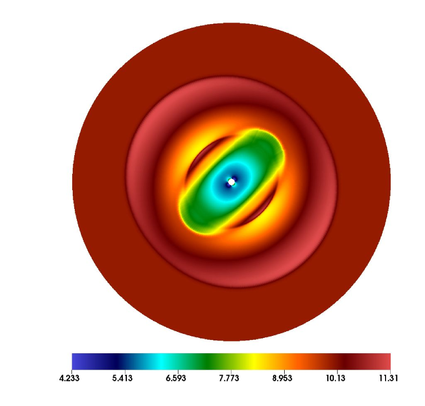
Figure 5: Magnetic field magnitude at time $t=0.07$ from the blast wave problem.

The methods described above are used without modification with the source term divergence cleaning algorithm (Eq. 6). However, the GLM method introduces two additional waves moving with the speeds $\pm c_{h}$ that carry changes in $B_{n}$ and $\psi$ only. Because $c_{h}$ is the fastest wave speed, these waves bound the “base” Riemann fan, comprised of 2, 3, or 5 waves in the HLLE, HLLC, and HLLD solvers, respectively. The intermediate states are readily obtained from the Rankine-Hugoniot conditions at the bounding waves as

$$B_{n}^{*}=\frac{B_{n,l}+B_{n,r}}{2}-\frac{\psi_{r}-\psi_{l}}{2c_{h}},$$

$$\psi^{*}=\frac{\psi_{l}+\psi_{r}}{2}-\frac{c_{h}(B_{n,r}-B_{n,l})}{2}.$$ (34)

These intermediate states serve as both the right and the left states for the actual Riemann solver. The advantage of this approach is that any possible jump in the normal component of $\mathbf{B}$ is taken up by these additional external waves.

Very few genuinely three-dimensional test problems are available for spherical grids. For code verification we used a 3D blast wave problem similar to those presented by Gardiner & Stone (2008) and Balsara et al. (2009). The simulation region is constrained between $r_{\mathrm{min}}=0.01$ and $r_{\mathrm{max}}=0.5$. The radial cell width $\Delta r$ increased outward monotonically from 0.00052 to 0.047. The inner boundary was treated as a perfectly conducting sphere with reflecting boundary conditions imposed. The initial conditions are $\rho=1$, $\mathbf{u}=0$, and $p=10\;(r<0.1)$, $p=0.1\;(r>0.1)$. The initial magnetic field is given by the standard potential solution for a perfectly conducting sphere in a uniform external field, namely

$$B_{r}=B_{0}\left(1-\frac{r_{\mathrm{min}}^{3}}{r^{3}}\right)\cos\theta,$$ (35)

$$B_{\theta}=-B_{0}\left(1+\frac{r_{\mathrm{min}}^{3}}{2r^{3}}\right)\sin\theta.$$ (36)

This solution was rotated such that the external field pointed in the direction $(1/\sqrt{3},1/\sqrt{3},1/\sqrt{3})$. We used $B_{0}=10$ and $\gamma=1.4$. The system was evolved until $t=0.07$.

For this problem we chose a level 6 grid with 256 cells in the radial direction. The GLM version of the numerical scheme was used with the HLLC Riemann solver and WENO reconstruction. Figure 5 shows the magnitude of magnetic field at the end of the simulation on a linear scale. The flow structure of the solution is qualitatively similar to Gardiner & Stone (2008) and Balsara et al. (2009), consisting of an outermost fast shock wave and two dense shells of material elongated along the magnetic field. This problem did not trigger the slope flattening or positivity correction routines meaning it is not a very good stress test of the code. Several more difficult problems simulating actual astrophysical plasma flows are discussed next.

6 Numerical solutions of test problems

To illustrate the capabilities of the new model we present results from three different simulations of solar system plasma environments. The first is a dynamic MHD simulation of compressive structures in the solar wind known as corotating interaction regions (CIRs). This is a simple test problem with a strong degree of spherical symmetry. The second is a simulation of the structure of the global heliosphere, including regions on each side of the interface between the solar wind and LISM known as the heliopause. This problem involves mode complex transonic flows and a population of neutral atoms in addition to the plasma. Finally, our third test problem is a stationary structure of the Earth’s magnetosphere. Unlike the two previous cases, this one is an example of a highly magnetized plasma environment.

6.1 Test problem 1: Corotating interaction regions in the solar wind

Corotating interaction regions (CIRs) are compressive structures produced through an interaction between high and low speed streams in the solar wind. CIRs are fully formed by the time they reach Earth’s orbit (Siscoe, 1972; Gosling et al., 1972). When the streams emanating from the Sun are approximately steady in the co-rotating frame, these compression regions form spirals in the solar equatorial plane that co-rotate with the Sun. The leading edge of a CIR is a forward compressional wave propagating into the slower solar wind ahead, whereas the tailing edge is a reverse wave propagating back into the trailing high speed stream. At large heliospheric distances the waves steepen into forward and reverse shocks. The entire plasma structure is convected with the solar wind and plays an important role in the dynamics of the heliosphere.

CIRs have been extensively studied using global MHD simulation (Pizzo, 1994; Riley et al., 2001; Usmanov & Goldstein, 2006). To generate CIRs in a global MHD simulation we adopt the tilted-dipole flow geometry of Pizzo (1982) at the inner boundary, which is illustrated in Figure 6. In this figure $0xyz$ is the fixed (heliographic) frame, where $z$ is the solar rotation axis, and $0x^{\prime}y^{\prime}z^{\prime}$ is a frame aligned with the Sun’s magnetic axis $z^{\prime}$. The parameter $\gamma$ is the dipole tilt angle, and $\beta$ is the latitude of the fast-slow transition boundaries (blue circles) in the coordinate system $0x^{\prime}y^{\prime}z^{\prime}$. In the simulation discussed below we used $\beta=\pm 30^{\circ}$.

Following Pogorelov et al. (2007), one readily derives a quadratic equation for the latitude of the transition line $\theta$ as a function of the azimuthal angle $\varphi$,

$$a\sin^{2}\theta+b\sin\theta+c=0,$$ (37)

where

$$a = \cos^{2}\gamma+\sin^{2}\gamma\tan^{2}\varphi(\cot\gamma\cos\gamma+\sin\gamma)^{2}$$

$$b = 2\sin\beta\cos\gamma(1+\tan^{2}\varphi)$$ (38)

$$c = \sin^{2}\beta(1+\tan^{2}\varphi\cos^{2}\gamma)-\cos^{2}\beta\sin^{2}\gamma\tan^{2}\varphi.$$

Note that when $\beta=0$, $\theta(\varphi)$ reduces to the expression for the latitude of the magnetic equator given by Eq. (A6) of Pogorelov et al. (2007).

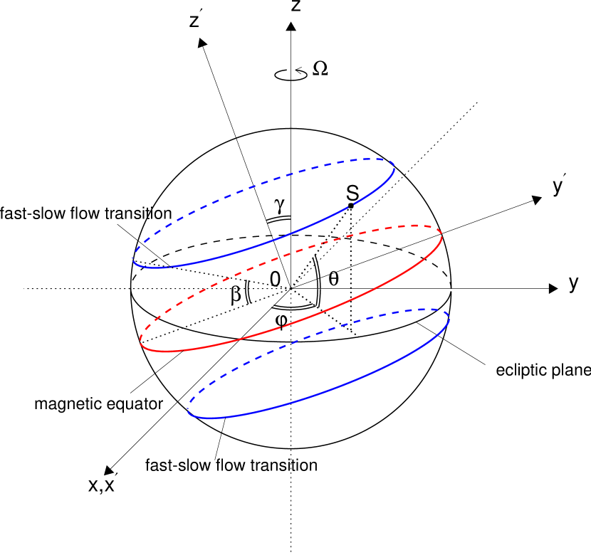
Figure 6: A diagram of the assumed titled-dipole plasma flow geometry for the CIR simulation.

We simulated a region of the solar wind between $r_{\mathrm{min}}=0.5$ AU and $r_{\mathrm{max}}=30$ AU using 512 concentric grid layers of variable thickness (increasing outward). At 1 AU we assume the following conditions: density $n=3.5$ cm^-3 and radial velocity $u=800$ km/s in the fast solar wind and $n=7$ cm^-3, $u=400$ km/s in the slow solar wind. The radial component of the magnetic field at 1 AU was $B_{r}=28$ $\mu$G. These conditions were extended to the inner boundary using the conventional Parker solution for the solar wind and its magnetic field (Parker, 1958). The dipole tilt angle was taken to be $\gamma=20^{\circ}$. The boundary (shear layer) between the fast and the slow solar wind flows was located at a latitude of $30^{\circ}$ in the coordinate system aligned with the dipole axis. This simulation was performed on a level 6 geodesic grid. We chose the HLLC solver to evolve the time-dependent MHD equations, combined with the GLM divergence cleaning method; WENO reconstructions was used in all directions.

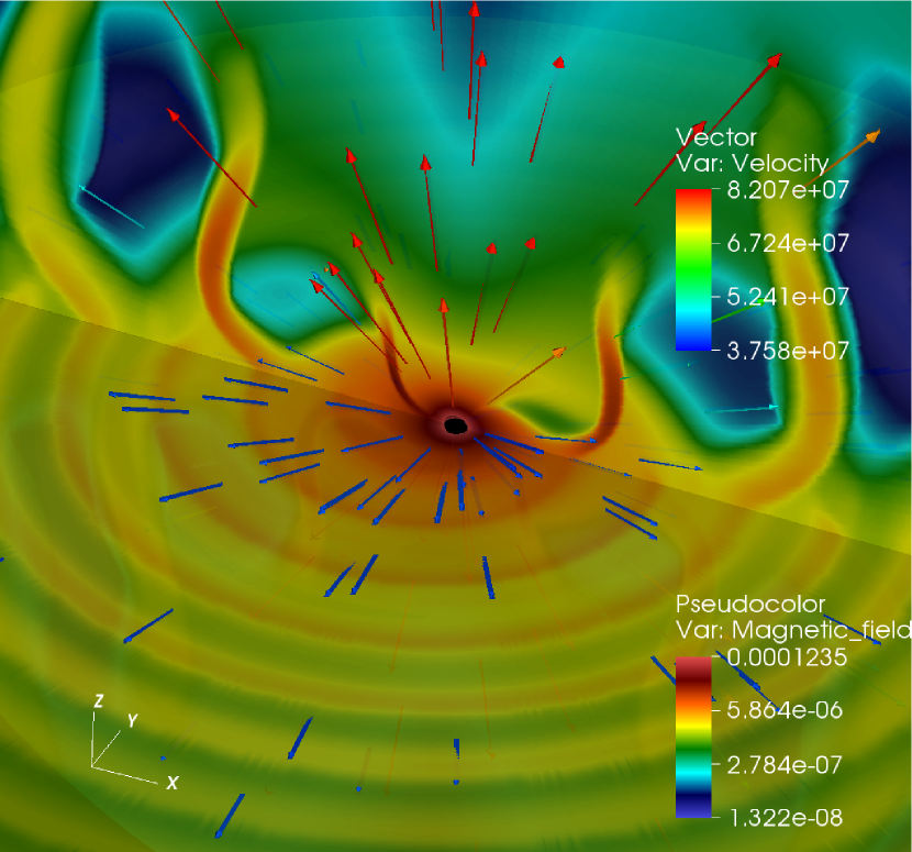
Figure 7: Left: Magnetic field magnitude (log scale) in the meridional plane ($xz$) and the solar equatorial plane ($xy$) for the CIR simulation. Arrows are the plasma velocity vectors. Right: radial profiles along the direction ($\theta$, $\varphi$) = ($25^{\circ}$, $135^{\circ}$) of (from top to bottom): plasma density (log scale), radial velocity, log thermal pressure, log magnetic field intensity, log temperature, and the north-south flow deflection angle $\epsilon$. Arrows mark the forward (pointing right) and reverse (pointing left) propagation of wave fronts.

Figure 7 (left) shows the logarithm of the magnetic field magnitude in the $xz$ and $xy$ planes using a cutout plot. Plasma velocity vectors are shown as arrows of variable length. The CIRs can be visually identified as higher density and magnetic field intensity regions (red). The maximum latitudinal extent of CIRs is given by the sum of the angle between the rotation and the dipole axes and the extent of the slow solar wind in the frame aligned with the dipole axis, i.e., $\gamma+\beta=50^{\circ}$. In the equatorial plane, the spiral CIR structure is seen to be bounded by shock-like discontinuities.

Several characteristic CIR features can be recognized in the plasma radial profiles shown in Figure 7 (right). We chose the profile along the direction $25^{\circ}$ northern latitude relative to the solar equatorial ($xy$) plane. The forward-reverse shock pairs are commonly observed at mid-latitudes, below the heliographic latitude of $26^{\circ}$ (Gosling & Pizzo, 1999). They are shown with vertical dashed lines in the Figure. Shock pairs associated with CIRs are believed to be responsible for the observed 26-day recurrent decreases in galactic cosmic-ray intensity (Kota & Jokipii, 1991; McKibben et al., 1999). Other features, such as the south-north flows are also identified through the north-south flow deflection angle $\epsilon=\sin^{-1}(-u_{\theta}/|\mathbf{u}|)$ shown in the bottom panel. The transitions from northward (positive) to southward (negative) velocity are separated by roughly one Carrington rotation period (26 days) in our simulation. We conclude that the model is capable of reproducing the essential CIR features and is consistent with the earlier simulations of this phenomenon.

6.2 Test problem 2: The global heliosphere

The energy density in a supersonic stellar wind, such as the solar wind, decreases in inverse proportion to the square of the distance from the star. Eventually the outflow is unable to maintain pressure balance with the galactic environment near the star, comprised mostly of partially ionized hydrogen gas. The stellar wind undergoes a transition to a subsonic flow at a structure called a termination shock. A tangential discontinuity called an astropause (heliopause for the solar wind) separates the shocked stellar flow from the interstellar gas. A bow shock may develop in front of the astropause if the relative motion between the star and LISM is supersonic. In the case of heliosphere, the region between the termination shock and the boundary is called the heliosheath. The theory of stellar wind interfaces (as applied primarily to the heliosphere) has been developed in Parker (1961), Axford (1972), and Baranov et al. (1976). Recent three-dimensional MHD simulations of the interface could be found in Pogorelov et al. (2007) and Opher et al. (2007).

To simulate the structure of the heliospheric interface we used a relatively coarse level 5 geodesic grid with 240 radial points. As in the CIR problem, the concentric layer spacing was nonuniform with the smallest cells at the inner radial boundary located at 10 AU; the outer boundary was placed at 900 AU. A heliographic coordinate system is used here, where the $z$ axis is aligned with the solar rotation axis (Beck & Giles, 2005), and the $x$ axis is in the plane formed by the $z$ axis and the interstellar helium flow direction (Lallement et al., 2005). The $y$ axis completes the right-handed orthogonal system. The geometry of the problem is illustrated in Figure 8.

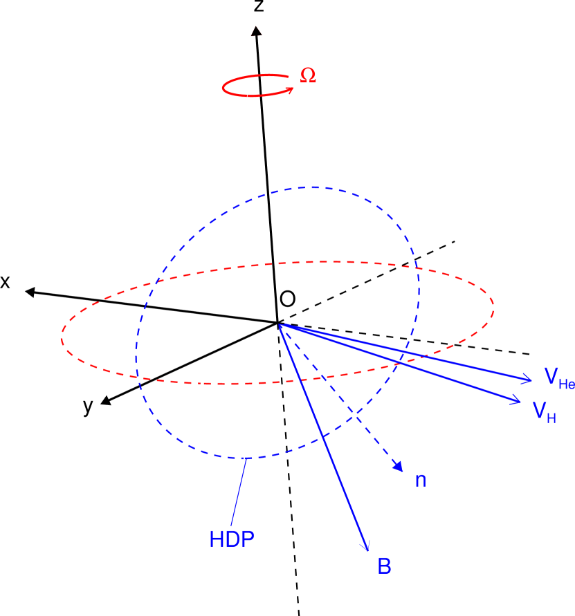
Figure 8: The heliographic coordinate system used in the simulation of the global heliosphere. The directions of the flow of interstellar hydrogen ($\mathbf{V}_{\mathrm{H}}$) and helium ($\mathbf{V}_{\mathrm{He}}$) span the so-called hydrogen deflection plane (HDP) with a normal $\mathbf{n}$. Here the interstellar magnetic field $\mathbf{B}$ lies in the HDP, with an angle of $45^{\circ}$ relative to $\mathbf{V}_{He}$.

The heliospheric configuration computed here is representative of a solar minimum (Florinski, 2011). At 1 AU we assume the following conditions: density $n=3.5$ cm^-3 and radial velocity $u=800$ km/s at heliographic latitudes above $30^{\circ}$ (fast solar wind) and $n=7$ cm^-3, $u=400$ km/s at low latitudes (slow solar wind). The magnetic field is a Parker spiral with a radial component $B_{r}=28$ $\mu$G at 1 AU. The azimuthal magnetic field component is a function of the solar wind speed. The heliospheric current sheet is not included in this simulation, so that the solar magnetic field is always directed outward from the Sun. The observed current sheet is between $10^{4}$ km (1 AU, Winterhalter et al., 1994) and a few times $10^{5}$ km (heliosheath, Burlaga & Ness, 2011) in width, which is much too narrow to be resolved with a global model.

The interstellar flow has a total density of 0.2 cm^-3, and is ionization rate of 0.25. Its velocity vector is $\mathbf{V}_{\mathrm{He}}=(-26.3,\,0,\,-0.23)$ km/s in the chosen heliographic coordinate system. The interstellar magnetic field lies in the so-called hydrogen deflection plane (the plane spanned by the velocity vectors of neutral interstellar hydrogen and helium) and is inclined by $45^{\circ}$ with respect to the LISM flow vector. Its components are $(-1.3,\,1.38,\,-2.32)$ $\mu$G in our coordinate system. The temperature of both ionized and neutral components in the LISM is taken to be 6530 K. The neutral and the plasma fluids are coupled via the charge exchange process (Axford, 1972). We simulate both fluids using the same code by explicitly fixing $\mathbf{B}=0$ for the neutral hydrogen. The charge exchange terms used are those of Pauls et al. (1995). For simplicity we only include interstellar hydrogen in this simulation and ignore atoms produced by charge exchange in the heliosheath or the solar wind. To separate the interstellar region from the heliosphere we use a passively advected indicator variable $q$ which satisfies the equation

$$\frac{\partial(\rho q)}{\partial t}+\nabla\cdot(\rho q\mathbf{u})=0.$$ (39)

The indicator variable is set to 1 in the solar wind and $-1$ in the interstellar flow. The condition $q=0$ then gives the location of the heliopause.

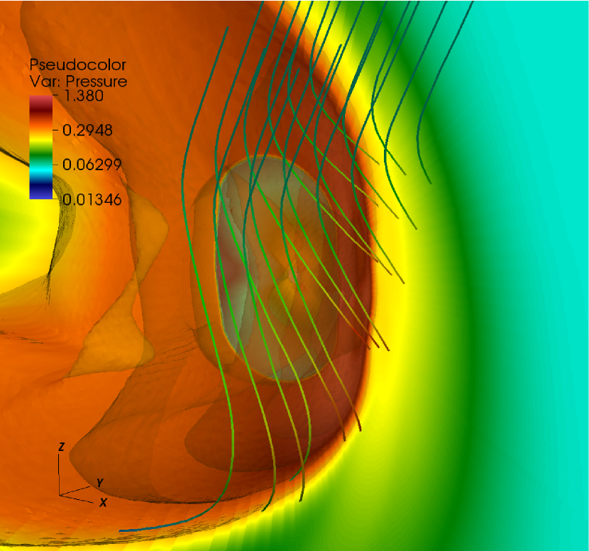
Figure 9: Left: Constant plasma pressure surfaces (log scale) cut by the meridional ($xz$) plane for the heliosphere simulation. Selected magnetic field lines in the LISM are shown. Right: Radial profiles in the upwind (nose) direction of (from top to bottom): log plasma number density, radial speed, log thermal pressure, magnetic field magnitude, and log temperature. The positions of the termination shock and the heliopause are marked with vertical dashed lines.

We chose the HLLC solver for this work because of its more robust handling of a strong flow shear between the fast and the slow solar wind. We used the GLM $\nabla\cdot\mathbf{B}$ control method and WENO reconstruction in all directions. Simulations were run until a steady state was achieved which took about 300 years of simulated time. Figure 9, left, shows a cutout view of the heliospheric interface. Surfaces of constant plasma pressure are plotted together with magnetic field lines in the LISM, illustrating their draping around the heliopause (the transition between the red and the green colors). The innermost pressure surface approximately traces the outline of the termination shock.

We show radial profiles of several physical quantities in the upwind, or “nose” direction in the right panel of Figure 9. Before the termination shock, located at 67 AU in this simulation, the solar wind velocity is gradually decreasing because of a loss of momentum to charge exchange with interstellar hydrogen. In the heliosheath, the plasma density is nearly a constant while the magnetic pressure increases toward the heliopause where the flow becomes essentially stagnant. The effective heliosheath temperature ($\sim 3\times 10^{6}$ K) is that of the solar-wind and pickup-ion mixture, which is significantly higher than that of the core solar wind ($\sim 2\times 10^{5}$ K, Richardson et al., 2008). From the top panel one can see that the density on the interstellar side of the heliopause is some 25 times higher than in the heliosheath. There is a very weak bow shock in this model barely visible in the pressure and temperature profiles.

The results presented here were obtained using a single population of neutral hydrogen (the interstellar atoms). The computer code is actually capable of integrating conservation laws for multiple neutral hydrogen populations. It would be straightforward to include the heliosheath energetic neutral atoms and the neutral solar wind atoms in a simulation, at an added computational time expense (e.g., Williams et al., 1997).

6.3 Test problem 3: Magnetosphere of Earth

The Earth’s magnetosphere is a product of an interaction between the supersonic solar wind and the geomagnetic field. Two major discontinuities, the bow shock and the magnetopause, are located between the undisturbed solar wind region and the geomagnetic field. The magnetosheath, filled with shocked solar wind plasma, lies between the bow shock and the magnetopause, which is the external boundary of the magnetosphere. The magnetopause thus separates the hot, tenuous magnetospheric plasma from the cold and dense solar wind plasma in the magnetosheath. Global MHD simulations, coupled with ionospheric models, have been widely used to study large-scale processes in the magnetosphere (e.g., Fedder & Lyon, 1995; Tanaka, 1995; Raeder, 1999; Hu et al., 2007).

The geomagnetic field can be treated as a dipole field in the inner magnetosphere, its strength varying as $r^{-3}$, where $r$ is the distance from the center of the Earth. The thermal pressure varies more modestly leading to a very low plasma $\beta$ (the ratio of the plasma thermal pressure to the magnetic field pressure) in the inner magnetosphere. Such low values of $\beta$ ($\sim 10^{-5}-10^{-4}$) tend to produce numerical errors with conservative numerical schemes (Raeder, 1999). To overcome this difficulty, the dipole field is treated apart from the total magnetic field according to the decomposition method introduced by Tanaka (1995). The momentum and energy fluxes in the Riemann solvers are revised accordingly. The WENO reconstruction method is used in all directions and the GLM algorithm is used to control $\nabla\cdot{\mathbf{B}}$. An interested reader will find more details on the GLM-MHD equations with a dipole field decomposition in the Appendix.

The Geocentric Solar Magnetospheric (GSM) coordinate system is used in this simulation. It is centered at Earth, and the $x$, $y$, and $z$ axes point to the Sun, the dawn-dusk direction, and along the north dipole axis, respectively. We choose the inner boundary to be a sphere with a radius $r=3R_{\mathrm{E}}$ (Earth radii), and apply the Dirichlet boundary conditions. In particular, the number density is 370 cm^-3, which is 1/27 of a typical value in the ionosphere. The thermal pressure is $4.65\times 10^{-10}$ dyn/cm², which is 9 times smaller than its ionospheric value. The magnetic field is taken to be a dipole field at the inner boundary. For the sake of simplicity, the magnetosphere-ionosphere electrostatic coupling (e.g., Janhunen, 1998) is not included, therefore the feedback of the ionosphere on the magnetosphere is ignored. We simply set the velocity to zero, which means there is no convection at the inner boundary. The free outer boundary is located at $r=100R_{E}$.

We simulate a common configuration with a southward interplanetary magnetic field (IMF) of 50 $\mu$G. The solar wind velocity is 600 km/s along the Sun-Earth line (the negative $x$ direction), its number density is 5 cm^-3 and temperature $9.1\times 10^{4}$ K. The magnetic field is initially calculated as a superposition of a dipole field, centered at the origin, and a mirror dipole, located at $(30R_{\mathrm{E}},\,0,\,0)$, The field on the sunward side is subsequently replaced with the solar wind field with $B_{z}=-50$ $\mu$G to make the initial configuration divergence free. In the simulation we used a level 6 geodesic grid and 256 grid points along the radial direction.

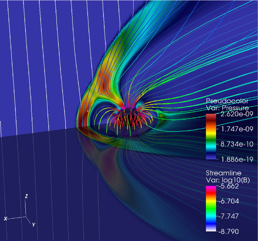
Figure 10: Left: plasma pressure (color) and magnetic field lines for the magnetosphere simulation. Plane cuts for $z=0$ and $y=0$ are shown. The magnitude of the magnetic field is shown by the color of the field lines in the figure. Right: radial profiles along the Sun-Earth line of (from top to bottom): log plasma number density, velocity, log thermal pressure, log magnetic field intensity, and log temperature. The bow shock and the magnetopause are marked by vertical dashed lines.

A steady state configuration is obtained some 30 minutes (simulated time) into the simulation. The left panel of Figure 10 shows the color contours of the thermal pressure in the meridional ($xz$) plane and in the equatorial ($xy$) plane. The geomagnetic field and the IMF lines of force are also plotted. In the equatorial plane the geomagnetic field points northward, being opposite to the polarity of the southward IMF. We can see that the magnetosphere is open to the interplanetary medium and the geomagnetic field lines connect with the IMF (Dungey, 1961). In that case the solar wind plasma momentum and energy can be transported into the magnetosphere through the site of magnetic reconnection. We did not observe surface waves or vortices induced by the Kelvin-Helmholtz instability (e.g., Guo et al., 2010) along the low-latitude magnetopause (the surface of the magnetopause is smooth in the equatorial plane).

The profiles of the physical quantities along the Sun-Earth line are shown in the right panel of Figure 10. The magnetopause is located at the neutral point for southward IMF case. The $x$ velocity component approaches zero at the subsolar point, where the Sun-Earth line intersects the magnetopause. The shocked plasma becomes dense and hot in the magnetosheath, compared with the undisturbed solar wind. For southward IMF, the neutral point is found from the magnetic field strength profile (fourth panel from the top), where magnetic reconnection could occur in the presence of dissipation.

Our result has all the relevant features of a typical MHD magnetospheric simulation. In this illustrative solution, we only calculate a steady state representative magnetosphere. Of course, the model can be also used with more realistic time-dependent IMF conditions derived from observations.

7 Summary

In this report we have presented a novel approach to numerical modeling of space plasma flows using geodesic spherical meshes with a nearly uniform solid angle coverage. This approach avoids the singularity on the symmetry axis inherent in polar spherical grids, leading to improved efficiency by allowing larger time steps. Our integration technique for gas-dynamic or MHD conservation laws is based on dimensionally unsplit time advance and uses two-dimensional reconstruction on the surface of a sphere. The new code has a number of useful features, such as a choice of multiple nonlinear Riemann solvers, weighted reconstruction limiters, and slope flattening to reduce possible oscillations near strong shocks.

We have tested the new model on several common problems in space physics: a formation of corotating interaction regions in the solar wind, global modeling of the heliospheric interface, and finally, the magnetosphere of a planet. Our results are consistent with those found in the literature and every feature of the resulting structures is well reproduced. At this time the model lacks an adaptive mesh refinement feature, which would permit a superior numerical resolution of shocks and discontinuities. Whereas a hexagonal (Voronoi) grid cannot be easily refined, its dual Delaunay grid can. The process starts with the original icosahedron that divides a sphere into 20 identical spherical triangles. Each triangle then may be recursively subdivided into four smaller triangles by connecting the midpoints of the original cell edges with great circle arcs. The Delaunay mesh is therefore naturally amenable to refinement based on an oct-tree formulation. Because each locally refined zone is further split in the radial direction, this is tantamount to each 3D patch giving rise to 8 identically-sized refined patches if it is to undergo one more level of refinement.

The model could be potentially adapted to solve problems where the compact object is not at the center of the region of interest. For example, following Tanaka (2000), one could introduce a non-concentric grid, where different spherical layer boundaries are offset from the origin. The offset distance increases for each subsequent layer, so that the mesh becomes denser in one direction and more rarefied in the opposite direction. Such an arrangement could be more efficient for modeling, e.g., a magnetosphere with a long tail.

The new code by itself could be a valuable tool to investigate plasma flows around a source whose dimensions are small compared with the scale of the flow. Nevertheless, its chief intended purpose is to provide plasma background for subsequent simulations of the transport of energetic charged particles in the solar system and other astrophysical environments. Additional modules, recently added to the code, calculate the diffusion coefficients and drift velocity vectors based on magnetic field and other plasma properties. The use of geodesic grids will permit a more efficient calculation of phase space trajectories in the stochastic integration method popular in cosmic-ray transport work (Ball et al., 2005; Florinski & Pogorelov, 2009). The difference with polar grid-based models is expected to be quite pronounced in the polar regions of the heliosphere, where the diffusion and drift coefficients are typically very large.

Appendix A Dipole field decomposition

In the magnetosphere, the external field $\mathbf{B}_{1}=\mathbf{B}-\mathbf{B}_{d}$, where $\mathbf{B}$ is the total magnetic field, and $\mathbf{B}_{d}$ is the internal dipole field. Since $\mathbf{B}_{d}$ is both curl-free (no current) and divergence free, we can write

$$\nabla\cdot\left(\mathbf{B}_{d}\mathbf{B}_{d}-\frac{1}{2}B_{d}^{2}{\mathbf{I}}\right)=0,$$ (A1)

$$(\nabla\times{\mathbf{B}_{d}})\cdot(\mathbf{u}\times\mathbf{B})=0.$$ (A2)

Using (A1) the momemtum flux from Eq. (4) can be expressed as

$$\rho{\mathbf{uu}}+p{\mathbf{I}}-\frac{1}{4\pi}\left(\mathbf{BB}+\frac{1}{2}B_{d}^{2}{\mathbf{I}}-\mathbf{B}_{d}\mathbf{B}_{d}\right).$$ (A3)

Next, from (A2) we obtain

$${\mathbf{B}_{d}}\cdot\nabla\times(\mathbf{u}\times\mathbf{B})-\nabla\cdot(\mathbf{u}\times\mathbf{B})\times{\mathbf{B}_{d}}=0,$$ (A4)

which, upon substitution into the magnetic induction equation

$$\frac{\partial\mathbf{B}}{\partial t}-\nabla\times(\mathbf{u}\times\mathbf{B})=0$$ (A5)

yields

$$\mathbf{B}_{d}\cdot\frac{\partial\mathbf{B}_{1}}{\partial t}-\nabla\cdot[\mathbf{B}(\mathbf{u}\cdot\mathbf{B}_{d})-\mathbf{u}(\mathbf{B}\cdot\mathbf{B}_{d})]=0.$$ (A6)

We now define

$$p_{1}^{*}=p_{g}+\frac{B_{1}^{2}}{8\pi},\quad e_{1}=\frac{\rho u^{2}}{2}+\frac{p_{g}}{\gamma-1}+\frac{B_{1}^{2}}{8\pi}.$$ (A7)

Using these definitions the energy equation may be written as

$$\frac{\partial e_{1}}{\partial t}+\frac{\mathbf{B}_{d}}{4\pi}\cdot\frac{\partial\mathbf{B}_{1}}{\partial t}+\nabla\cdot\left\{(e_{1}+p_{1}^{*}){\mathbf{u}}\right.$$

$$\left.+\frac{1}{4\pi}[\mathbf{u}(\mathbf{B}_{1}\cdot\mathbf{B}_{d})+\mathbf{u}(\mathbf{B}\cdot\mathbf{B}_{d})-\mathbf{B}(\mathbf{u}\cdot\mathbf{B}_{1})-\mathbf{B}(\mathbf{u}\cdot\mathbf{B}_{d})]\right\}=0.$$ (A8)

Combining equations (A6) and (A8) yields

$$\frac{\partial e_{1}}{\partial t}+\nabla\cdot\left\{(e_{1}+p_{1}^{*}){\mathbf{u}}-\frac{1}{4\pi}[\mathbf{B}_{1}(\mathbf{u}\cdot\mathbf{B}_{1})-\mathbf{u}(\mathbf{B}_{d}\cdot\mathbf{B}_{1})+\mathbf{B}_{d}(\mathbf{u}\cdot\mathbf{B}_{1})]\right\}=0.$$ (A9)

Using (A3) and (A9) the system of GLM-MHD equations with dipole field decomposition may be written as

$$\frac{\partial\rho}{\partial t}+\nabla\cdot(\rho{\mathbf{u}})=0,$$ (A10)

$$\frac{\partial(\rho{\mathbf{u}})}{\partial t}+\nabla\cdot\left[\rho{\mathbf{uu}}+p^{*}{\mathbf{I}}-\frac{1}{4\pi}\left({\mathbf{BB}}+\frac{1}{2}B_{d}^{2}{\mathbf{I}}-\mathbf{B}_{d}\mathbf{B}_{d}\right)\right]=0,$$ (A11)

$$\frac{\partial{\mathbf{B}_{1}}}{\partial t}+\nabla\cdot({\mathbf{uB}-\mathbf{Bu}+\psi{\mathbf{I}}})=0,$$ (A12)

$$\frac{\partial e_{1}}{\partial t}+\nabla\cdot\left\{(e_{1}+p_{1}^{*}){\mathbf{u}}-\frac{1}{4\pi}\left[(\mathbf{u}\cdot\mathbf{B}_{1})\mathbf{B}_{1}-(\mathbf{B}_{d}\times\mathbf{u})\times\mathbf{B}_{1}\right]\right\}=0,$$ (A13)

$$\frac{\partial\psi}{\partial t}+c_{h}^{2}\nabla\cdot\mathbf{B}_{1}=-\frac{c_{h}^{2}}{c_{p}^{2}}\psi,$$ (A14)

Note that the system (A10)–A(14) uses $\mathbf{B}_{1}$ and $e_{1}$ instead of $\mathbf{B}$ and $e$ as conserved quantities

Consider the simplest three-state HLL solver (Harten et al., 1983). Its Riemann flux is given by

$$\mathbf{F}=\left\{\begin{array}[]{ll}\mathbf{F}_{l},&S_{l}>0,\\ \mathbf{F}_{lr},&S_{l}\leq 0\leq S_{r},\\ \mathbf{F}_{r},&S_{r}<0,\end{array}\right.$$ (A15)

where $\mathbf{F}_{l}=\mathbf{F}(\mathbf{U}_{l})$ and $\mathbf{F}_{r}=\mathbf{F}(\mathbf{U}_{r})$ are the left and right unperturbed fluxes, respectively. The intermediate flux $\mathbf{F}_{lr}$ is given by

$$\mathbf{F}_{lr}=\frac{S_{r}\mathbf{F}_{l}-S_{l}\mathbf{F}_{r}+S_{l}S_{r}(\mathbf{U}_{r}-\mathbf{U}_{l})}{S_{r}-S_{l}}.$$ (A16)

Since only the definition of a conserved flux is required to solve (A15), the system (A10)–(A14) can be readily used in place of (4).

The decomposition of magnetic field does not affect the GLM scheme. For example, in the $x$ direction we have two GLM equations,

$$\frac{\partial B_{1x}}{\partial t}+\frac{\partial\psi}{\partial x}=0,$$ (A17)

$$\frac{\partial\psi}{\partial t}+\frac{\partial(c_{h}^{2}B_{1x})}{\partial x}=-\frac{c_{h}^{2}}{c_{p}^{2}}\psi.$$ (A18)

One can see that the external field component $B_{1x}$ can be integrated directly because the internal field ($\mathbf{B}_{d}$ related terms) does not appear in these equations.

References

- Axford (1972) Axford, W. I. 1972, in NASA Special Pub. 308, Solar Wind, ed. C. P. Sonnett, et al. (Washington, DC: NASA) 609
- Balsara (2010) Balsara, D. S., 2010, J. Comput. Phys., 229, 1970
- Balsara (2012) Balsara, D. S., 2012, J. Comput. Phys., doi:10.1016/j.jcp.2011.12.025
- Balsara et al. (2009) Balsara, D. S., Rumpf, T., Dumbser, M., & Munz, C.-D. 2009, J. Comput. Phys., 228, 2480
- Ball et al. (2005) Ball, B., Zhang, M., Rassoul, H., & Linde, T. 2005, ApJ, 634, 1116
- Baranov et al. (1976) Baranov, V. B., Krasnobaev, K. V., & Ruderman, M. S. 1976, Ap&SS, 41, 481
- Batten et al. (1997) Batten, P., Clarke, N., Lambert, C., & Causon, D. M. 1997, SIAM J. Sci. Comput., 18, 1553
- Beck & Giles (2005) Beck, J. G., & Giles, P. 2005, ApJ, L153
- Burlaga & Ness (2011) Burlaga, L. F., & Ness, N. F. 2011, J. Geophys. Res., 116, A051012
- Christov & Popov (2008) Christov, I., & Popov, B. 2008, J. Comput. Phys., 227, 5736
- Dedner et al. (2002) Dedner, A., Kemm, F., Kröner, D., Munz, C.-D., Schnitzer, T., & Wesenberg, M. 2002, J. Comput. Phys., 175, 645
- Du et al. (2003) Du, Q., Gunzburger, M. D., & Ju, L. 2003, Comput. Methods Appl. Mech. Engrg., 192, 3933
- Dungey (1961) Dungey, J. W. 1961, Phys. Rev. Lett., 6, 47
- Einfeldt et al. (1991) Einfeldt, B., Munz, C. D., Roe, P. L., & Sjögreen, B. 1991, J. Comput. Phys., 92, 273
- Fedder & Lyon (1995) Fedder, J. A., & Lyon, J. G. 1995, J. Geophys. Res., 100, 3623
- Florinski (2011) Florinski, V. 2011, Adv. Space Res., 48, 308
- Florinski & Pogorelov (2009) Florinski, V., & Pogorelov, N. V. 2009, ApJ, 701, 642
- Friedrich (1998) Friedrich, O. 1998, J. Comput. Phys., 144, 194
- Gardiner & Stone (2008) Gardiner, T. A., & Stone, J. M. 2008, J. Comput. Phys., 227, 4123.
- Gosling et al. (1972) Gosling, J. T., Hundhausen, A. J., Pizzo, V., & Asbridge, J. R. 1972, J. Geophys. Res., 77, 5442
- Gosling & Pizzo (1999) Gosling, J. T., & Pizzo, V. J. 1999, Space Sci. Rev., 89, 21
- Guo et al. (2010) Guo, X. C., Wang, C., & Hu, Y. Q. 2010, J. Geophys. Res., 115, A10218
- Gurski (2004) Gurski, K. F. 2004, SIAM J. Sci. Comput., 25, 2165
- Harten et al. (1983) Harten, A., Lax, P. D., & van Leer, B. 1983, SIAM Rev., 25, 35
- Heikes & Randall (1995) Heikes, R., & Randall, D. A. 1995, Mon. Weather Rev., 123, 1862
- Hu et al. (2007) Hu, Y. Q., Guo, X. C., & Wang, C. 2007, J. Geophys. Res., 112, A07215
- Janhunen (1998) Janhunen, P. 1998, Ann. Geophys., 16, 397
- Kota & Jokipii (1991) Kota, J., & Jokipii, J. R. 1991, J. Geophys. Res., 18, 1979
- Lallement et al. (2005) Lallement, R., Quemerais, E., Bertaux, J. L., Ferron, S., Koutroumpa, D., & Pellinen, R. 2005, Science, 307, 1447
- Li (2005) Li, S. 2005, J. Comput. Phys., 203, 344
- McKibben et al. (1999) McKibben, R. B., Jokipii, J. R., Burger, R. A., Heber, B., Kota, J., McDonald, F. B., Paizis, C., Potgieter, M. S., & Richardson, I. G. 1999, Space Sci. Rev., 89, 307
- Miyoshi & Kusano (2005) Miyoshi, T., & Kusano, K. 2005, J. Comput. Phys., 208, 315
- Nakamizo et al. (2009) Nakamizo, A., Tanaka, T., Kubo, Y., Kamei, S., Shimazu, H., & Shinagawa, H. 2009, J. Geophys. Res., 114, A07109
- Opher et al. (2007) Opher, M., Stone, E. C., & Gombosi, T. I. 2007, Science, 316, 875
- Parker (1958) Parker, E. N. 1958, ApJ, 128, 664
- Parker (1961) Parker, E. N. 1961, ApJ, 134, 20
- Pauls et al. (1995) Pauls, H. L., Zank, G. P., & Williams, L. L. 1995, J. Geophys. Res., 100, 21,595
- Pizzo (1982) Pizzo, V. J. 1982, J. Geophys. Res., 87, 4374
- Pizzo (1994) Pizzo, V. J. 1994, J. Geophys. Res., 99, 4173
- Pogorelov & Matsuda (1998) Pogorelov, N. V., & Matsuda, T. 1998, J. Geophys. Res., 103, 237
- Pogorelov et al. (2007) Pogorelov, N. V., Stone, E. C., Florinski, V., & Zank, G. P. 2007, ApJ, 668, 611
- Powell et al. (1999) Powell, K. G., Roe, P. L., Linde, T. J., Gombosi, T. I., & De Zeeuw, D. L. 1999, J. Comput. Phys., 154, 284
- Putman & Lin (2007) Putman, W. M., & Lin, S.-J. 2007, J. Comput. Phys., 227, 55
- Raeder (1999) Raeder, J. 1999, J. Geophys. Res., 104, 17,357
- Ratkiewicz et al. (1998) Ratkiewicz, R., Barnes, A., Molvik, G. A., Spreiter, J. R., Stahara, S. S., Vinokur, M., & Venkateswaran, S. 1998, A&A, 335, 363
- Richardson et al. (2008) Richardson, J. D., Kasper, J. C., Wang, C., Belcher, J. W., & Lazarus, A. J. 2008, Nature, 454, 63
- Riley et al. (2001) Riley, P., Linker, J. A., & Mikic, Z. 2001, J. Geophys. Res., 106, 15,889
- Ronchi et al. (1996) Ronchi, C., Iacono, R., & Paolucci, P. S. 1996, J. Comput. Phys., 124, 93
- Siscoe (1972) Siscoe, G. L. 1972, J. Geophys. Res., 77, 27
- Tanaka (1995) Tanaka, T. 1995, J. Geophys. Res., 100, 12057
- Tanaka (2000) Tanaka, T. 2000, J. Geophys. Res., 105, 21,081
- Tóth et al. (1998) Tóth, G., Keppens, R., & Botchev, M. A. 1998, A&A, 332, 1159
- Upadhyaya et al. (2010) Upadhyaya, H. C., Sharma, O. P., Mittal, R., & Fatima, H. 2010, Asia-Pac. J. Chem. Eng., doi: 10.1029/apj.479
- Usmanov & Goldstein (2006) Usmanov, A. V., & Goldstein, M. L. 2006, J. Geophys. Res., 111, A07101
- van Leer (1977) van Leer, B. 1977, J. Comput. Phys., 23, 276
- Washimi & Tanaka (1996) Washimi, H., & Tanaka, T. 1996, Space Sci. Rev., 78, 85
- Williams et al. (1997) Williams, L. L., Hall, D. T., Pauls, H. L., & Zank, G. P. 1997, ApJ, 476, 366
- Winterhalter et al. (1994) Winterhalter, D., Smith, E. J., Burton, M. E., Murphy, N., & McComas, D. J. 1994, J. Geophys. Res., 99, 6667
- Yeh (2007) Yeh, K-S. 2007, J. Comput. Phys., 225, 1632