Stability of thin liquid films and sessile droplets under confinement

Abstract

The stability of nonvolatile thin liquid films and of sessile droplets is strongly affected by finite size effects. We analyze their stability within the framework of density functional theory using the sharp kink approximation, i.e., on the basis of an effective interface Hamiltonian. We show that finite size effects suppress spinodal dewetting of films because it is driven by a long-wavelength instability. Therefore nonvolatile films are stable if the substrate area is too small. Similarly, nonvolatile droplets connected to a wetting film become unstable if the substrate area is too large. This instability of a nonvolatile sessile droplet turns out to be equivalent to the instability of a volatile drop which can atttain chemical equilibrium with its vapor.

I Introduction

Dewetting of fluid films and the ensuing formation of sessile droplets are both part of everyday experience. Moreover these mechanisms are important for the functioning of biological systems as well as for numerous technological processes. Dewetting on homogeneous substrates and the subsequent formation of droplets have been studied both experimentally reiter01a ; seemann01b ; seemann01d ; becker03 ; muellerbuschbaum03 ; fetzer05 ; fetzer07b ; hamieh07 ; ralston08 and theoretically bausch94b ; BeGrWi00 ; thiele01c ; glasner03a ; blossey06a ; vilmin06b ; bertrand07 ; deconinck08 in great detail. Both mechanisms can be understood quantitatively within the well established theory of wetting phenomena degennes85 ; dietrich88 ; rauscher08a ; rauscher10a . More recently, wetting and dewetting on structured surfaces receives increasing attention, in particular with a view on controlling the dewetting process on patterned surfaces jackman98 ; lipowsky00 ; kargupta01a ; kargupta02a ; brusch02 ; thiele03a ; harkema03 ; checco12 as well as in the context of microfluidics dietrich05 ; squires05a ; delamarche05 ; koplik06a ; rauscher07a ; mechkov08 . Chemical patterns consisting of lyophilic and lyophobic patches as well as topographic patterns such as pits and grooves effectively lead to a lateral confinement of wetting films and droplets.

It is well known that confinement modifies the structural and thermodynamic properties of condensed matter. In small scale systems these finite size effects can either stabilize or destabilize certain structures. For example, systems exhibiting a long-wavelength instability are characterized by a critical wavelength such that fluctuations with larger wavelengths grow exponentially in time. This type of instability is suppressed in systems smaller than this critical wavelength. On the other hand, certain structures can only exist if they are larger than a certain critical size, such as droplets which, at least within classical nucleation theory, have to be larger than the critical nucleus. This means that certain structures are suppressed by finite size effects, or, to put it differently, the availability of large space can stabilize them.

Spinodally unstable flat films show a long-wavelength instability such that the dependence of their stability on the substrate size is obvious. Droplets of nonvolatile fluids, however, are usually considered to be stable. But they are in chemical equilibrium with an adsorbate or a wetting film connected to them degennes85 ; dietrich88 ; rauscher08a ; rauscher10a which, on very large substrates, acts like a reservoir: a spherical droplet of $100$ nm radius has the same volume as an adsorbate layer with an effective thickness of 1 Å on a substrate of $6.5\times 6.5\,\mu\mathrm{m}^{2}$. Therefore, an isolated droplet of a nonvolatile fluid placed on a macroscopically large substrate is expected to be unstable with respect to the formation of a film. If a droplet is volatile, i.e., in chemical equilibrium with its vapor, it is expected to be unstable, too, but with respect to evaporation or condensation and the formation of an equilibrium wetting layer.

The Laplace pressure in droplets decreases upon increasing their diameter while the pressure in wetting films is determined by the disjoining pressure. In the case of stable films it increases with their thickness. In a stationary situation the pressure in the droplet is balanced by the pressure in the connected film. Moving a small amount of fluid from a droplet into its attached film increases the pressure in the drop and, as the thickness of the film increases, also the pressure in the film. However, due to volume conservation, the larger the substrate the smaller is the increase of the ensuing film thickness and therefore the smaller is the increase of pressure in the film. This implies, that beyond a certain substrate size the pressure increase in the drop is larger than the pressure increase in the film and the drop will dissipate into the large film mechkov08 .

On the other hand, a substrate of limited size can only support droplets with a base radius smaller than half the substrate diameter. This means, that one can expect that there is a window of droplet sizes for stable droplets as shown for two-dimensional droplets with small slopes (i.e., liquid ridges with a small contact angle) in Ref. dutka12 . Since droplet volumes scale with the third power of the droplet radius while the volume of the wetting or adsorbate film scales with the second power of the substrate diameter, the influence of the wetting or adsorbate film on droplet stability is most important on the nanoscale because in this case the volumes of the liquid in the droplet and in the film are comparable. In addition, due to the non-vanishing width of the three-phase-contact line there is a minimal size for well defined droplets burschka93 ; bausch94b , which gives rise to an additional contribution to the finite size effects.

In this spirit, here we study the influence of substrate size on the stability of flat films and of droplets using the framework of density functional theory within the sharp kink approximation, i.e., by minimizing the corresponding effective interface Hamiltonian dietrich91b in the presence of an effective interface potential dietrich91a ; napiorkowski92 .

II Effective interface Hamiltonian

Within the capillary model for nonvolatile fluids rowlinson02 ; safran03 ; brochardwyart04 interfaces and contact lines are geometrical objects of zero volume and area, respectively, and the free energy of a fluid in contact with a substrate is given by bulk, interface, and line contributions which are proportional to the volume, interface areas, and contact line lengths, respectively. Within this macroscopic model, finite size effects occur only if the three-phase-contact line of a droplet reaches the lateral boundary of the substrate. Wetting transitions and the dependence on temperature and pressure of the thickness of wetting layers cannot be described within this macroscopic model.

For this reason, in order to access mesoscopic scales, we resort to the effective interface model as the simplest non-trivial model to describe a fluid in contact with a substrate. It can be derived from a classical density functional theory using the so-called sharp-kink approximation dietrich91b ; napiorkowski93 . As in the capillary model, also in this approach interfaces are only two-dimensional manifolds but contact lines, such as the three-phase-contact line between fluid, vapor, and substrate have a nonzero width as a result of explicitly taking into account the finite range of intermolecular interactions (for reviews see Refs. rauscher08a ; rauscher10a ). Accordingly, within this model line tensions emerge and are not input parameters indekeu92 ; dobbs93 ; indekeu94a ; getta98 ; bauer99b ; bauer00a ; schimmele07 .

The effective, local interface Hamiltonian $\mathcal{H}$ for a liquid film in Monge parameterization $z=h(x,y)$ on a homogeneous substrate with the substrate-liquid interface $A$ located in the $xy$-plane reads

$$\mathcal{H}[h]=\int_{A}dx\,dy\,\bigg{[}\sigma\,\sqrt{1+(\partial_{x}h)^{2}+(\partial_{y}h)^{2}}\\ +\,\phi(h)+\delta\mu\,h\bigg{]},$$ (1)

with the liquid-gas interface tension $\sigma$. $\phi(z)$ is the effective interface potential dietrich88 ; dietrich91a ; napiorkowski92 and it describes the effective interaction between the liquid-vapor interface and the liquid-substrate interface. The last term $\delta\mu=\Delta\rho\,\Delta\mu$ is the product of the undersaturation $\Delta\mu=\mu_{\mathrm{coexistence}}(T)-\mu$ at temperature $T$ and the number density difference $\Delta\rho=\rho_{\mathrm{liquid}}-\rho_{\mathrm{vapor}}$ between the coexisting phases, and thus it measures the thermodynamic distance from the bulk two-phase coexistence line. Within mean field theory the equilibrium configuration of the liquid-vapor interface minimizes $\mathcal{H}[h]$.

The Monge parameterization is restricted to single valued interface configurations $z=h(x,y)$ so that droplets with contact angles larger than $90^{\circ}$ cannot be described this way. Therefore we rewrite Eq. (1) in a parameter free form also used in the finite element code employed below. For arbitrary parameterizations of the liquid-gas interface $\mathbf{r}(u,v)=(x(u,v),y(u,v),z(u,v))$ the area of the surface element is $d\mathbf{A}=\frac{\partial\mathbf{r}}{\partial u}\times\frac{\partial\mathbf{r}}{\partial v}\,du\,dv=G\,\mathbf{\hat{n}}\,du\,dv$ with the interface normal vector $\mathbf{\hat{n}}$ pointing into the gas phase and $G=\left|\frac{\partial\mathbf{r}}{\partial u}\times\frac{\partial\mathbf{r}}{\partial v}\right|$. In the Monge parameterization this reduces to $G=\sqrt{1+|\bm{\nabla}h(\mathbf{r})|^{2}}$, i.e., the first term in the square brackets in Eq. (1). The effective interface Hamiltonian can be written in terms of an integral over the liquid-vapor interface $S$

$$\mathcal{H}[\mathbf{r}]=\int_{S}d\mathbf{A}\cdot\left\{\sigma\,\mathbf{\hat{n}}(u,v)+\left[\phi(z(u,v))+\delta\mu\,z(u,v)\right]\,\mathbf{\hat{e}}_{z}\right\},$$ (2)

with $\mathbf{\hat{e}}_{z}$ as the normal vector of the substrate-liquid interface pointing into the liquid phase, i.e., in $z$-direction.

The existence of a classical density functional has been proven for grand canonical ensembles evans79 . Nonetheless the functional in Eq. (1) has been used successfully to describe also equilibrium shapes of nonvolatile fluids (i.e., in the canonical ensemble) by fixing the liquid volume $V$ via a Lagrange multiplier $p$. In this case, $\delta\mu$ is not an independent parameter. It turns out, that upon adding the constant term $\delta\mu\,V$ (which is independent of the droplet shape) to the functional in Eq. (1), $\delta\mu$ and $p$ multiply the same terms such that $\delta\mu$ can be absorbed into $p$. It will turn out later (see Eq. (7)) that $p$ is the pressure difference between the liquid and the vapor, and for droplets one has $p>0$, given the choice of sign for the Lagrange multiplier contribution as in Eq. (3). Since in a nonvolatile system the liquid and the vapor are not in thermodynamic equilibrium, the pressures do not have to be equal. This leads to a variation principle for the equilibrium shape of the liquid-vapor interface of nonvolatile fluids. The equilibrium shape $\mathbf{r}^{(\text{eq})}(u,v)$ minimizes the functional ($\int_{S}d\mathbf{A}\cdot\mathbf{\hat{e}}_{z}=A$)

$$\mathcal{F}[\mathbf{r}(u,v)]=\int_{S}d\mathbf{A}\cdot\bigg{\{}\sigma\,\mathbf{\hat{n}}(u,v)+\\ \left[\phi(z(u,v))-p\,\left(z(u,v)-\frac{V}{A}\right)\right]\,\mathbf{\hat{e}}_{z}\bigg{\}}.$$ (3)

In the case of the laterally homogeneous substrates considered in this paper, the effective interface potential $\phi(z)$ does not explicitly depend on the lateral coordinates $(x,y)$. However, due to the formation of droplets one can still find non-trivial solutions to the minimization problem in Eq. (3). The structure of $\phi(z)$ depends on the types of intermolecular interactions involved. The simplest effective interface potential for long-ranged dispersion forces (described by Lennard-Jones type interactions) and at temperatures below the wetting temperature has the form

$$\phi(z)=\phi_{0}\,\left(\frac{h_{0}^{8}}{3\,z^{8}}-\frac{4\,h_{0}^{2}}{3\,z^{2}}\right).$$ (4)

The potential has a minimum of depth $-\phi_{0}$ at $z=h_{0}$ and an inflection point at $z=h_{i}\equiv\sqrt[6]{3}\,h_{0}\approx 1.2\,h_{0}$ (see Fig. 1). The potential is negative for $z>\sqrt[3]{1/2}\,h_{0}$ and approaches zero from below for $z\to\infty$. The shape of $\phi(z)$ corresponds to that of a continuous wetting transition dietrich88 .

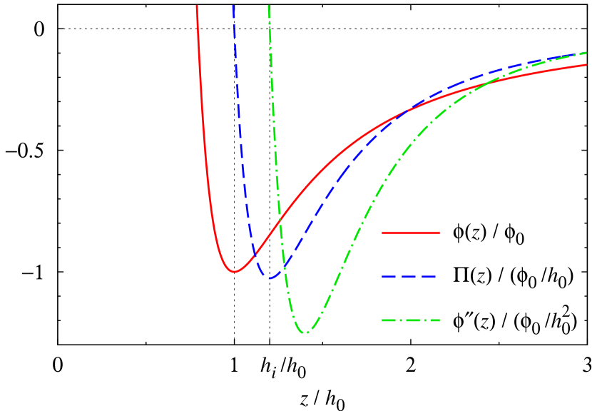
Figure 1: The effective interface potential $\phi(z)$ (full red line) according to Eq. (4) and the corresponding disjoining pressure $\Pi(z)=-\phi^{\prime}(z)$ (dashed blue line) in units of $\phi_{0}$ and $\phi_{0}/h_{0}$, respectively. The positions of the minimum of $\phi(z)$ at $z=h_{0}$ and of its inflection point at $z=h_{i}\equiv\sqrt[6]{3}\,h_{0}\approx 1.2\,h_{0}$ are indicated by vertical dotted lines. Also shown is $\phi^{\prime\prime}(z)$ (dash-dotted green line) which appears in the second variation operator $\hat{O}_{h}$ in Eq. (10) and which determines the stability of flat film solutions (see Eq. (17)).

II.1 Minimizing the free energy functional

Within mean-field theory the minimum of the effective interface functional $\mathcal{F}$ containing the volume constraint (Eq. (3)) renders the interfacial free energy for the corresponding stable equilibrium configuration.

The functional in Eq. (3) can be minimized numerically by means of an adaptive finite element algorithm implemented by the software Surface Evolver brakke92 . Therein, the liquid-vapor interface is represented by a mesh of oriented triangles and, by means of a gradient projection method, iteratively evolves towards the configuration of minimal $\mathcal{F}$ (for an example see Fig. 2) below.

II.2 Variations of the effective interface Hamiltonian

Within the framework of variational calculus, a stable equilibrium profile corresponds to a vanishing first variation and a negative second variation of the functional $\mathcal{F}$. In order to calculate them we return to the Monge parameterization and introduce the perturbed interface configuration $z=\tilde{h}(x,y)$ with $\tilde{h}(x,y)=h(x,y)+\epsilon\,\Psi(x,y)$ and $\tilde{p}=p+\epsilon\,\psi$, where $0<\epsilon\ll 1$ is a small dimensionless parameter. It is straightforward to show that the first variation $\delta^{(1)}\mathcal{F}$ of $\mathcal{F}([\tilde{h}],\tilde{p})=\mathcal{F}([h],p)+\epsilon\,\delta^{(1)}\mathcal{F}+\epsilon^{2}\,\delta^{(2)}\mathcal{F}+\mathcal{O}(\epsilon^{3})$ with respect to the interface configuration is given by ($h=h(x,y)$)

$$\delta^{(1)}\mathcal{F}=\int_{A}dx\,dy\,\Psi\,\left[-2\,\sigma\,H_{h}+\phi^{\prime}(h)-p\right]\\ +\psi\,\int_{A}dx\,dy\,\left(h-\frac{V}{A}\right),$$ (5)

with the mean curvature

$$H_{h}=\frac{(\partial_{x}^{2}h)\,[1+(\partial_{y})^{2}]-2\,(\partial_{x}h)\,(\partial_{y}h)\,(\partial_{x}\partial_{y}h)+(\partial_{y}^{2}h)\,[1+(\partial_{x}h)^{2}]}{2\,\sqrt{1+(\partial_{x}h)^{2}+(\partial_{y}h)^{2}}^{3}}$$ (6)

of the unperturbed surface and $\phi^{\prime}(h)$ denoting the derivative of the effective interface potential with respect to the local film thickness. The Euler-Lagrange equation corresponding to the vanishing of $\delta^{(1)}\mathcal{F}$ is

$$2\,\sigma\,H_{h}+\Pi(h)+p=0$$ (7)

together with

$$V=\int_{A}dx\,dy\,h,$$ (8)

where $\Pi(h)=-\phi^{\prime}(h)$ is the disjoining pressure, which describes the effective interaction between the substrate surface and the film surface, and $2\,\sigma\,H_{h}$ is the Laplace pressure, which follows from the interface tension of the fluid surface. For equilibrium interface configurations the sum of the disjoining pressure and of the Laplace pressure is constant. The variation with respect to the Lagrange multiplier $p$ leads to the volume constraint (see Eq. (8)).

The second variation $\delta^{(2)}\mathcal{F}$ of $\mathcal{F}$ with respect to the film height can be written as a form quadratic in the perturbation $\Psi$:

$$\delta^{(2)}\mathcal{F}=\int_{A}dx\,dy\,\left(\Psi\,\hat{O}_{h}\,\Psi+2\,\psi\,\Psi\right),$$ (9)

with the self-adjoined operator

$$\hat{O}_{h}=-\sigma\,\left(\begin{array}[]{c}\partial_{x}\\ \partial_{y}\end{array}\right)\cdot\left(\begin{array}[]{cc}\frac{1+(\partial_{y}h)^{2}}{\left[1+(\partial_{x}h)^{2}+(\partial_{y}h)^{2}\right]^{\frac{3}{2}}}&\frac{(\partial_{x}h)\,(\partial_{y}h)}{\left[1+(\partial_{x}h)^{2}+(\partial_{y}h)^{2}\right]^{\frac{3}{2}}}\\ \frac{(\partial_{x}h)\,(\partial_{y}h)}{\left[1+(\partial_{x}h)^{2}+(\partial_{y}h)^{2}\right]^{\frac{3}{2}}}&\frac{1+(\partial_{x}h)^{2}}{\left[1+(\partial_{x}h)^{2}+(\partial_{y}h)^{2}\right]^{\frac{3}{2}}}\end{array}\right)\cdot\left(\begin{array}[]{c}\partial_{x}\\ \partial_{y}\end{array}\right)+\phi^{\prime\prime}(h),$$ (10)

and with the second derivative $\phi^{\prime\prime}(h)$ of the effective interface potential. For the model potential given in Eq. (4) $\phi^{\prime\prime}(h)$ is shown in Fig. 1. It is positive for small $h$ and negative for large $h$. The second variation with respect to the Lagrange multiplier is identical to zero. The mixed variation with respect to $p$ and $h$ leads to the second term in Eq. (9) which due to $\psi=\textit{const.}$ vanishes for perturbations $\Psi(x,y)$ which conserve the volume. The stability of a solution of the Euler-Lagrange equation (7) is determined by the spectrum of eigenvalues of $\hat{O}_{h}$. A solution is linearly stable if all eigenvalues are positive.

III Thin films and nano-droplets

On a chemically homogeneous substrate with an area $A$ there exist two distinct classes of solutions of the Euler-Lagrange equation (7). One consists of flat films with

$$h^{(\text{eq})}(x,y)=h_{f}=V/A.$$ (11)

The other class consists of nontrivial droplet solutions with one or many droplets smoothly connected to a wetting film. Here we focus on solutions with a single droplet because in general two or more droplets connected via a wetting film are unstable with respect to coarsening. In the following we discuss the stability of flat films and such droplets as a function of the substrate area $A$, of the excess liquid volume

$$V_{\mathrm{ex}}=V-A\,h_{0}=(h_{f}-h_{0})\,A,$$ (12)

and of material properties encoded in $\phi(h)/\sigma$.

III.1 Flat films

For flat films with homogeneous thickness $h_{f}$ the Euler-Lagrange equation (7) reduces to

$$p+\Pi(h_{f})=0.$$ (13)

This means that for any size of the substrate area a homogeneous flat film obeying Eq. (13) is obviously a solution of the Euler-Lagrange equation. It represents either a local maximum, a local minimum, or a saddle point of the free energy functional in Eq. (3). The curvature of the interface is zero and thus the liquid gas interface tension drops out. If $h_{f}$ minimizes the effective interface potential one has $p=0$ (assuming that $\phi(h)$ is differentiable). For a flat interface the operator $\hat{O}_{h}$ in Eq. (10), which determines the linear stability of the flat film solution, reduces to

$$\hat{O}_{h}=-\sigma\,(\partial_{x}^{2}+\partial_{y}^{2})+\phi^{\prime\prime}(h_{f}).$$ (14)

The corresponding eigenvalue problem has the form of a stationary single particle Schrödinger equation with a potential which is constant across the domain of the substrate. In Fig. 1 $\phi^{\prime\prime}(z)$ is shown for the model potential from Eq. (4). The inverse surface tension plays the role of the mass.

The eigenvalue spectrum of this operator depends on the shape of the domain and on the boundary conditions at its borders. Boundary conditions corresponding to actual substrates of finite size are rarely compatible with a flat film solution because usually there is a bending of the interface at the edge of the domain. For example, at the edge of a lyophilic patch on a lyophobic substrate the film thickness will go to zero (or at least to a microscopically small value) and at the brim of a flat piece of substrate the fluid film either continues onto the side walls or ends with thickness zero. The two simplest types of mathematical boundary conditions, which allow for flat film solutions, are either periodic boundary conditions or a Neumann type boundary condition which corresponds to zero slope of the film surface at the domain boundaries. The latter would correspond to upright side walls with an equilibrium wetting angle of $90^{\circ}$ at a pit-shaped substrate. However, even for such a setup, the interplay of the long-ranged forces from the substrate and from the side wall would lead to a bending of the film surface moosavi06b ; moosavi09 .

For a square substrate with edge length $L=\sqrt{A}$ and with Neumann boundary conditions the eigenvalue problem corresponding to $\hat{O}_{h}$ can be factorized by separating the variables and the eigenfunctions are given by plane waves. The degeneracy of the eigenfunctions characterized by wave vectors of equal modulus is alleviated by the boundary condition. Assuming the two edges of the substrate to be aligned with the $x$-axis and with the $y$-axis, respectively, the eigenfunctions are given by

$$\Psi_{nm}(x,y)\propto\ \cos\left(\tfrac{2\,\pi\,n}{L}\,x\right)\,\cos\left(\tfrac{2\,\pi\,m}{L}\,y\right),$$ (15)

with $n,m\in\mathbb{N}_{0}$. Since $\Psi_{(-n)m}=\Psi_{n(-m)}=\Psi_{(-n)(-m)}=\Psi_{nm}$ we only consider non-negative indices. Since we consider a nonvolatile system there is volume conservation, i.e., $\int_{A}dx\,dy\,\Psi_{nm}=0$ and therefore either $n$ or $m$ have to be positive. The corresponding eigenvalues are given by

$$\lambda_{nm}=\sigma\,\left(\tfrac{2\,\pi}{L}\right)^{2}\,\left(n^{2}+m^{2}\right)+\phi^{\prime\prime}(h_{f})\/.$$ (16)

Therefore the film is linearly stable, i.e., $\min\limits_{n,m}\lambda_{nm}>0$, for

$$\frac{(2\,\pi)^{2}}{A}>-\frac{\phi^{\prime\prime}(h_{f})}{\sigma}.$$ (17)

For substrates of infinite, i.e., macroscopic, size $A$ this is the case only if $\phi^{\prime\prime}(h_{f})>0$. For the model effective interface potential in Eq. (4) the latter inequality holds for

$$h_{f}<h_{i}\equiv\sqrt[6]{3}\,h_{0}\approx 1.2\,h_{0},$$ (18)

Since $h_{i}>h_{0}$ (see Fig. 1) films with negative excess volumes (i.e., $h_{f}<h_{0}$ (see Eq. (12))) exhibit $\phi^{\prime\prime}(h_{f})>0$ so that, according to Eq. (17), they are linearly stable for any substrate size $A=L^{2}$. However, even for $\phi^{\prime\prime}(h_{f})<0$ flat films are linearly stable if the substrate size $L$ is below the critical value $L_{c}=2\,\pi\,\sqrt{\sigma/|\phi^{\prime\prime}(h_{f})|}$. This perturbation analysis does not yield any information about the nonlinear stability of film solutions, i.e., whether a flat film has a lower free energy than a droplet.

III.2 The nano-droplet configuration

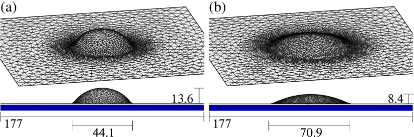
Figure 2: Interface configurations $h^{(\text{eq})}$ of nano-droplets as obtained by numerical minimization of the functional $\mathcal{F}$ in Eq. (3) based on the effective interface potential in Eq. (4) for $A/(\pi\,h_{0}^{2})=100^{2}$ and under the constraint $V_{\mathrm{ex}}/(A\,h_{0})=0.5$, with $\phi_{0}/\sigma=0.5$ ($\theta_{\mathrm{eq}}=60^{\circ}$, left panel (a)), and $\phi_{0}/\sigma=0.1$ ($\theta_{\mathrm{eq}}=26^{\circ}$, right panel (b)). In the projected side view (bottom row), the underlying substrate of area $A$ is indicated in blue. Lengths are given in units of $h_{0}$. Drop heights are measured from above the wetting film thickness $h_{w}^{(\text{eq})}=1.009\,h_{0}$ in (a) and $h_{w}^{(\text{eq})}=1.012\,h_{0}$ in (b). During the iterative minimization process, the mesh size of the triangulation has been coupled to the evolution of the interface shape in an adaptive way in order to optimize the spatial resolution locally. The lateral boundary conditions are implemented by a constraint on the boundary vertices, such that their lateral coordinates are fixed during the minimization process while the perpendicular height coordinate can evolve freely, effectively corresponding to neutral wetting (contact angle $90^{\circ}$) at vertical side walls (not shown) or Neumann boundary conditions.

For a given area $A$ and a certain ratio $V_{\mathrm{ex}}/(A\,h_{0})$ (see Eq. (12)), nano-droplets with a nonzero pressure $p>0$ minimize the free energy $\mathcal{F}$ in Eq. (3). This is due to the interplay of the surface free energy densities and the effective interface potential, in combination with the non-volatility of the liquid and the finite area $A$ of the solid-liquid interface. Since the difference between the liquid-substrate and the gas-substrate surface tensions is given by $\sigma+\phi(h_{0})$ Young’s law young05 reads dietrich88 :

$$\cos\theta_{\mathrm{eq}}=1-\frac{\phi_{0}}{\sigma}.$$ (19)

$\theta_{\mathrm{eq}}$ denotes the equilibrium contact angle of a macroscopic drop. The influence of the ratio $\phi_{0}/\sigma$ on the shape of a nano-droplet is shown in Fig. 2. A suitable definition of the contact angle of a nano-droplet is to determine the curvature of its surface at the apex, to inscribe the corresponding cap of a sphere which intersects the asymptote of the attached wetting film thus forming a contact angle schimmele07 . For the systems studied here, this contact angle is smaller than $\theta_{\mathrm{eq}}$.

The wetting film surrounding the nano-droplet is almost flat, i.e., $2\,\sigma\,|H_{h}|\ll|\Pi(h)|$ (see Eq. (7)). According to this Euler-Lagrange equation (7), the spatially constant pressure $p$ is approximately given by

$$p\approx-\Pi(h_{w}^{(\text{eq})}),$$ (20)

and thus $h_{w}^{(\text{eq})}>h_{0}$ implies $p>0$ (see Fig. 1).

The height $h_{w}^{(\text{eq})}$ of the wetting film, the pressure $p$, the disjoining pressure $\Pi(h_{w}^{(\text{eq})})$ of the wetting film, and the ratio between the drop free energy $\mathcal{F}_{\text{drop}}$ and the free energy $\mathcal{F}_{\text{film}}$ of a flat film with the same excess volume are shown in Table 1 for several values of $V_{\mathrm{ex}}$. For decreasing values of $V_{\mathrm{ex}}/(A\,h_{0})$ with constant $A$, $p$ increases. This is mainly due to the increasing curvature of the liquid-vapor interface. For the same reason the pressure in macroscopic drops also increases with decreasing volume. While the free energy $\mathcal{F}_{\text{drop}}$ of large drops turns out to be smaller than the free energy $\mathcal{F}_{\text{film}}$ of a flat film with the same excess volume, the situation is reversed for $V_{\mathrm{ex}}/(A\,h_{0})<0.06$ (the critical excess volume lies between $0.05\,A\,h_{0}$ and $0.06\,A\,h_{0}$). This means that nano-droplets below a certain size become metastable or unstable.

$V_{\mathrm{ex}}/(A\,h_{0})$	$h_{w}^{(\text{eq})}/h_{0}-1$	$p\,h_{0}/\sigma$	$-\Pi(h_{w}^{(\text{eq})})\,h_{0}/\sigma$	$\mathcal{F}_{\text{drop}}/\mathcal{F}_{\text{film}}$
0.05	0.0263	0.1777	0.1779	1.0003
0.06	0.0219	0.1526	0.1522	0.9975
0.10	0.0166	0.1191	0.1192	0.9782
0.20	0.0125	0.0922	0.0922	0.9130
0.50	0.0091	0.0674	0.0684	0.7730

Table 1: Characteristics of nano-droplets obtained via numerical minimization of $\mathcal{F}$ in Eq. (3) based on Eq. (4) for $A/(\pi\,h_{0}^{2})=100^{2}$ and $\phi_{0}/\sigma=0.5$; $h_{w}^{(\text{eq})}$ is the height of the film at the edge of the numerical domain. The pressure $p$ as the value of the Lagrange multiplier for fixing the volume and the disjoining pressure $\Pi(h_{w}^{(\text{eq})})$ of the wetting film surrounding the droplet as calculated from the numerically determined $h_{w}^{(\text{eq})}$ are balanced according to Eq. (20). Accordingly, the differences between the third and fourth column indicate the level of numerical accuracy. $\mathcal{F}_{\text{drop}}/\mathcal{F}_{\text{film}}$ is the ratio of the (mean-field) surface free energy of a nano-droplet and the free energy of a flat film with a height $h_{f}=V_{\mathrm{ex}}/A+h_{0}$.

III.3 Morphological transition

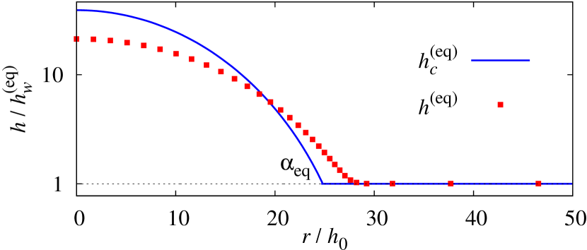
Figure 3: Vertical cut through the apex of a fully numerically obtained interface profile $h^{(\text{eq})}$ (red squares) and the corresponding approximate profile $h^{(\text{eq})}_{c}$ (full blue line) consisting of a spherical cap resting on a flat film. The profiles correspond to $A/(\pi\,h_{0}^{2})=100^{2}$, $V_{\mathrm{ex}}/(A\,h_{0})=0.5$, and $\phi_{0}/\sigma=0.5$, which are the parameters corresponding to Fig. 2(a) and to the bottom line in Table 1. Although the domain for the numerical calculation is rectangular, the droplet shape is to a good approximation radially symmetric ($r=\sqrt{x^{2}+y^{2}}$). The wetting film height for both profiles is $h_{w}^{(\text{eq})}=1.01\,h_{0}$ and the contact angle is $\alpha_{\mathrm{eq}}=55^{\circ}$ compared with $\theta_{\mathrm{eq}}=60^{\circ}$ for the corresponding macroscopic drop. The free energies for these profiles agree up to the third digit.

In order to analyze the morphological phase transition between nano-droplets and flat films as indicated by the numerical data discussed above, we minimize the effective interface Hamiltonian $\mathcal{F}$ in Eq. (3) in the subspace of interface shapes $h_{c}(x,y)$ describing a spherical cap sitting on top of a flat wetting film (see Fig. 3). For a given total volume of liquid, these trial profiles are parameterized by the contact angle $\alpha$ and the wetting film height $h_{w}$. The latter determines the fluid volume available for the drop connected to the film and the contact angle determines the drop shape. This ansatz reduces the problem of minimizing $\mathcal{F}$ in Eq. (3) to a minimization problem of the function

$$F(\alpha,h_{w})=\mathcal{F}[h_{c}(x,y)]$$ (21)

depending on the two variables $\alpha$ and $h_{w}$ with the minimum at $\alpha_{\mathrm{eq}}$ and $h_{w}^{(\text{eq})}$. The corresponding minimizing profile is denoted by $h_{c}^{(\text{eq})}$. In contrast to the direct, full numerical minimization of the free energy functional in Eq. (3), the function $F(\alpha,h_{w})$ provides also a free energy landscape in the parameter space $(\alpha,h_{w})$. Since for these two-parameter trial functions the wetting film is perfectly flat, the Laplace pressure vanishes and instead of Eq. (20) one has

$$p=-\Pi(h_{w}^{(eq)}).$$ (22)

In the macroscopic limit, i.e., upon increasing both $A$ and $V_{\mathrm{ex}}$ such that

$$\frac{A}{h_{0}^{2}}\to\infty\quad\text{with}\quad\frac{V_{\mathrm{ex}}}{A\,h_{0}}=\text{const}$$ (23)

one finds $h_{w}^{(\text{eq})}\to h_{0}$ for the droplet solution because in this limit the Laplace pressure $2\,\sigma\,H_{h}$ as well as the disjoining pressure at the cap apex vanish. The reason for this is that the curvature of the droplet surface goes to zero if the drop size diverges and that the disjoining pressure vanishes for large distances from the substrate surface. Therefore the sum of the disjoining pressure and of the Laplace pressure, i.e., $-p$, also vanishes (see Eq. (7)). The Lagrange multiplier $p$ does not depend on the position along the droplet surface and, according to Eq. (22), the disjoining pressure on the wetting film is also zero. Therefore a macroscopic liquid cap with volume $V_{\mathrm{ex}}$ is formed above the level $h_{w}^{(\text{eq})}=h_{0}$ where $\Pi(h_{0})=0$. The numerical minimization of $F(\alpha,h_{w})$ also yields, in this limit, $\alpha_{\mathrm{eq}}\to\theta_{\mathrm{eq}}$ with $\theta_{\mathrm{eq}}$ given by Eq. (19). Figure 4 shows the free energy landscape $F(\alpha,h_{w})$ for a large drop. All points in the parameter space $\{\alpha,(h_{w}-h_{0})/(h_{f}-h_{0})<1\}$ correspond to droplet solutions (see Eq. (11)), i.e., $\alpha\neq 0$. The line $(h_{w}-h_{0})/(h_{f}-h_{0})=1$ corresponds to a flat film solution for which $F(\alpha,h_{w})$ is independent of $\alpha$ because the volume of the droplet is zero. The global minimum of the free energy is located at $\alpha_{\mathrm{eq}}\approx\theta_{\mathrm{eq}}=60^{\circ}$ and $h_{w}^{(\text{eq})}\approx h_{0}$. The contour lines of the free energy landscape close to the minimum in Fig. 4 are almost parallel to the $\alpha$ axis and hence shape fluctuations of the liquid cap with a constant cap volume are more likely than volume fluctuations, i.e., fluctuations of the wetting film height $h_{w}$. As shown in the inset of Fig. 4 the equilibrium angle $\alpha_{\mathrm{eq}}$ approaches the macroscopic equilibrium contact angle $\theta_{\mathrm{eq}}$ from below.

In Fig. 4 the excess volume is chosen such that $h_{f}<h_{i}$, i.e., according to Eq. (18) the film configuration is linearly stable. Nonetheless, the droplet solution is the global minimum of $F(\alpha,h_{w})$. However, as shown in Fig. 5(a) there is a minimal droplet size $V_{\mathrm{ex}}$ below which droplets cannot exist: reducing the droplet size the Laplace pressure in the droplet increases until it cannot be counterbalanced by the negative disjoining pressure $-p=\Pi(h_{w}^{eq})$ (see Eq. (22)) in the film ($\Pi(z)$ has a minimum of finite depth (see Fig. 1)) and the droplet drains into the film. In Fig. 5(a) there is also a second branch of droplet solutions which are unstable and which have a pressure $p$ intermediate between the pressure of the metastable or stable droplets and of the flat film. For a given value of $V_{\mathrm{ex}}$ such a droplet solution corresponds to the saddle point in the two-dimensional parameter space between the two (local) minima given by the droplet solution and the flat film solution. Upon reaching the macroscopic limit, the unstable droplet branch asymptotically approaches the flat film pressure from below (Fig. 5(a)). This means, that the thickness $h_{w}^{(\text{eq})}$ of the wetting film surrounding the unstable droplets approaches the thickness $h_{f}=V_{\mathrm{ex}}/A+h_{0}$ of the flat film solution. Therefore the volume inside the unstable droplets (i.e., above $h_{w}$) decreases monotonically as the macroscopic limit is approached. Figure 5 corresponds to Fig. 12 in Ref. dutka12 where, however, the volume rather than the pressure is plotted as a function of the substrate size without discussing the stability of the solutions. We conclude that in this respect in essence there is no qualitative difference between the quasi two-dimensional ridges studied in Ref. dutka12 and the three-dimensional systems studied here.

For large excess volumes with $h_{f}>h_{i}$, according to Eq. (18), the flat film solution is linearly unstable. Therefore it should represent a saddle point or a maximum in the free energy landscape. The droplet solution should represent the global minimum. However, as shown in Fig. 5(b) the flat film solution for $h_{f}=1.25\,h_{0}>h_{i}$ is either stable or metastable, but not unstable within this only two-dimensonal parameter space considered here. In addition there is an unphysical branch of unstable droplet solutions with pressures above the pressure of the flat film solution. The reason for this artefact is, that a slightly undulated film cannot be represented in this two-dimensional parameter space; but spinodal dewetting occurs via the growth of such small perturbations. According to Eq. (17), the critical substrate size, below which the instability is suppressed by the finite size effects, is $\sqrt{A/(\pi\,h_{0}^{2})}\approx 6$, i.e., much smaller than $\sqrt{A/(\pi\,h_{0}^{2})}\approx 11.2$, the smallest substrate size for which the present two-dimensional parameter space analysis predicts the existence of droplet solutions (see Fig. 5(b)). In view of this inconsistency we conclude that the results obtained within this approximate scheme for very small substrate sizes are unreliable. However, the actual stability of droplets in the macroscopic limit is correctly covered within this model.

At the morphological transition a flat film and a droplet of equal volume have the same free energy but different pressure. In the theory of thermodynamic phase transitions, it is common to consider transitions between states of different volume (or density) but equal pressure (or more general, between states with equal intensive state variables but distinct extensive ones). These states can spatially coexist with each other. However, the morphological transition between a flat film and a droplet is of a different nature in the sense that the droplet solution and the flat film solution do not coexist with each other in space: the system as a whole switches from one solution to the other. This is not to be confused with the coexistence between a droplet and the wetting film to which it is connected. While the pressure in the wetting film and the pressure in the droplet are equal, this droplet configuration does not represent a bona fide thermodynamic phase: its pressure changes with size whereas from a proper thermodynamic phase one would expect to be able to produce systems of different size but with the same pressure. In fact, Eq. (1) has the structure of a Ginzburg-Landau Hamiltonian but the potential $\Phi(h)$ has its second minimum at $h\to\infty$. In this sense the droplet as a whole amounts to an interfacial region.

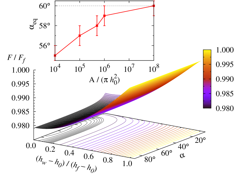
Figure 4: The approximate interfacial free energy $F(\alpha,h_{w})$ close to the macroscopic limit as described by Eq. (23): $A/(\pi\,h_{0}^{2})=10^{8}$, $V_{\mathrm{ex}}/(A\,h_{0})=0.06$, and for $\phi_{0}/\sigma=0.5$ corresponding to $\theta_{\mathrm{eq}}=60^{\circ}$. $F_{f}=A\,(\sigma+\phi(h_{f}))$ is the free energy of the flat film solution for these parameters; $h_{f}-h_{0}=V_{\mathrm{ex}}/A$. The global minimum is located at $\alpha\approx\theta_{\mathrm{eq}}=60^{\circ}$ and $h_{w}\approx h_{0}$. The contour lines are almost parallel to the $\alpha$-axis. (The contour lines shown range from $0.9792$ to $0.98$ in steps of $0.0001$ and from $0.98$ to $1.0$ in steps of $0.001$.) The inset shows the equilibrium angle $\alpha_{\mathrm{eq}}$ upon approaching the macroscopic limit as described by Eq. (23) for the same excess volume as used in the main figure; $\alpha_{\mathrm{eq}}$ approaches $\theta_{\mathrm{eq}}$ from below. The error bars are due to numerical inaccuracies. With $h_{f}/h_{0}=V_{\mathrm{ex}}/(A\,h_{0})+1=1.06<h_{i}/h_{0}=1.2$ (see Eq. (18)) the flat film solution with $(h_{w}-h_{0})/(h_{f}-h_{0})=1$ is expected to be linearly stable (i.e., metastable). But the number of data points calculated here is to small in order to be able to detect the corresponding free energy barrier (cf. Fig. 9 for a smaller substrate).

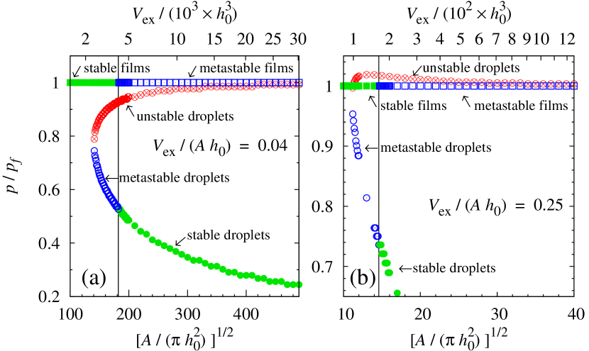
Figure 5: The pressure $p=-\Pi(h_{w}^{(\text{eq})})$ (see Eq. (22)) (in units of $p_{f}=-\Pi(h_{f})$) calculated from the approximate free energy in Eq. (21) as a function of the substrate size $A$ and of the excess volume $V_{\mathrm{ex}}$ for (a) $V_{\mathrm{ex}}/(A\,h_{0})=0.04$ and (b) $V_{\mathrm{ex}}/(A\,h_{0})=0.25$, i.e., for a fixed homogeneous film thickness $h_{f}=1.04\,h_{0}<h_{i}$ and $h_{f}=1.25\,h_{0}>h_{i}$, respectively, and $\phi_{0}/\sigma=0.5$. Note that for a fixed ratio $V_{\mathrm{ex}}/(A\,h_{0})=v_{\text{ex}}$ one has $V_{\mathrm{ex}}/h_{0}^{3}=\pi\,v_{\text{ex}}\,x^{2}$ with $x=[A/(\pi\,h_{0}^{2})]^{1/2}$. Open blue and full green symbols indicate metastable and stable states, respectively, and circles with crosses indicate unstable droplet solutions. Stable and metastable flat film solutions are indicated by boxes and stable and metastable droplets by circles. The vertical line indicates the morphological transition between stable films and stable droplets as obtained via numerical comparison of the corresponding two free energies. (A Maxwell construction for determining this transition point is discussed in, cf., Fig. 11.) $A\to\infty$ corresponds to the macroscopic limit. (a) For $h_{f}<h_{i}$, as in the present case corresponding to $V_{\mathrm{ex}}/(A\,h_{0})=0.04$, the flat film solution is stable or metastable for all $A$. Droplets (lowest branch) occur for $\sqrt{A/(\pi\,h_{0}^{2})}\gtrsim 140$ and they are stable for $\sqrt{A/(\pi\,h_{0}^{2})}\gtrsim 180$. (b) Within the present free energy approximation, the flat film solution is stable or metastable (although it should be unstable according to Eq. (18)) and there is an unphysical unstable branch of droplet solutions (top branch). Droplets are stable or metastable for for all substrate sizes $A$.

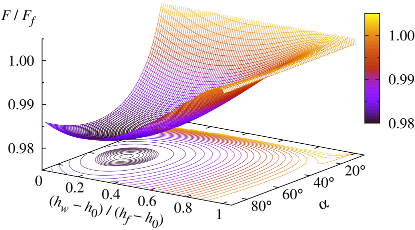
Figure 6: The approximate interfacial free energy $F(\alpha,h_{w})$ for $A/(\pi h_{0}^{2})=100^{2}$, $V_{\mathrm{ex}}/(A\,h_{0})=0.10$, and $\phi_{0}/\sigma=0.5$. $F_{f}=A\,(\sigma+\phi(h_{f}))$ is the free energy of the flat film solution for these parameters; $h_{f}-h_{0}=V_{\mathrm{ex}}/A$. The global minimum representing a stable nano-droplet is located at $(h_{w}^{(\text{eq})}-h_{0})/(h_{f}-h_{0})\approx 0.2$ and $\alpha_{\mathrm{eq}}\approx 57^{\circ}$, i.e., close to but smaller than the macroscopic equilibrium contact angle $\theta_{\mathrm{eq}}=60^{\circ}$ for this system. The flat film solution $h_{w}^{(\text{eq})}=h_{f}$ (so that $(h_{w}^{(\text{eq})}-h_{0})/(h_{f}-h_{0})=1$) is metastable; for this solution there is no dependence on $\alpha$. Contour lines are shown in the range $0.9802$ to $0.9809$ in steps of $0.0001$ and from $0.981$ to $1.005$ in steps of $0.001$.

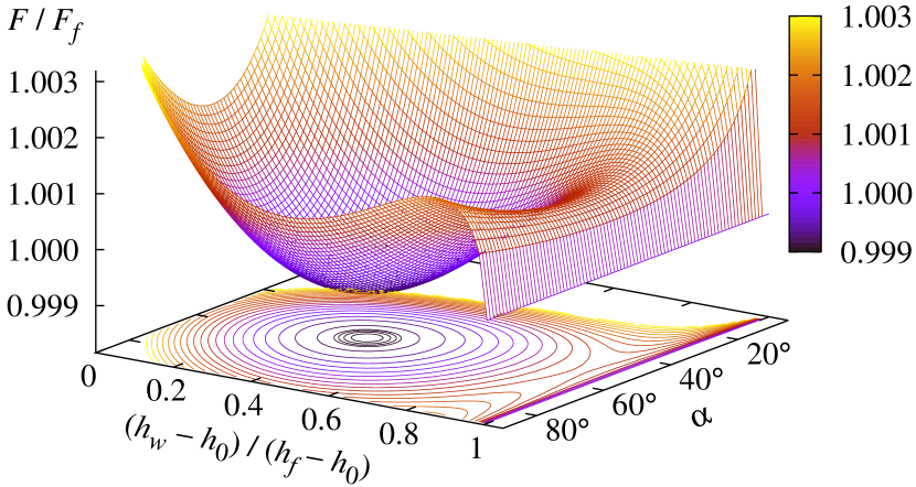
Figure 7: The approximate free energy $F(\alpha,h_{w})$ as defined in Eq. (21) for $A/(\pi h_{0}^{2})=100^{2}$, $V_{\mathrm{ex}}/(A\,h_{0})=0.06$, and $\phi_{0}/\sigma=0.5$ (i.e., for the same parameters as in Fig. 6 but for a smaller value of $V_{\mathrm{ex}}$). $F_{f}=A\,(\sigma+\phi(h_{f}))$ is the free energy of the flat film solution for these parameters; $h_{f}-h_{0}=V_{\mathrm{ex}}/A$. The contact angle corresponding to the global minimum is $\alpha_{\mathrm{eq}}\approx 55^{\circ}$ at $(h_{w}^{(\text{eq})}-h_{0})/(h_{f}-h_{0})\approx 0.04$, i.e., smaller than in Fig. 6. The flat film solution $h_{w}^{(\text{eq})}=h_{f}$ (so that $(h_{w}^{(\text{eq})}-h_{0})/(h_{f}-h_{0})=1$) is metastable and exhibits no dependence on $\alpha$. Contour lines are shown in the range $0.99902$ to $0.9991$ in steps of $0.00002$ and from $0.9992$ to $1.003$ in steps of $0.0002$.

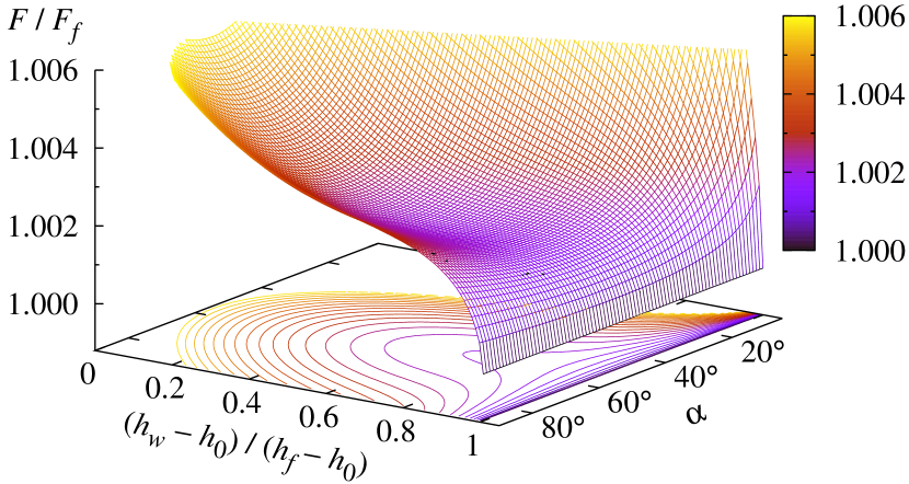
Figure 8: The approximate interfacial free energy $F(\alpha,h_{w})$ for $A/(\pi h_{0}^{2})=100^{2}$, $V_{\mathrm{ex}}/(A\,h_{0})=0.048$, and $\phi_{0}/\sigma=0.5$ (i.e., for the same parameters as in Figs. 6 and 7 but for a smaller value of $V_{\mathrm{ex}}$). $F_{f}=A\,(\sigma+\phi(h_{f}))$ is the free energy of the flat film solution for these parameters; $h_{f}-h_{0}=V_{\mathrm{ex}}/A$. For this excess volume the droplet solution has disappeared and the flat film solution $h_{w}^{(\text{eq})}=h_{f}$ (so that $(h_{w}^{(\text{eq})}-h_{0})/(h_{f}-h_{0})=1$) is the global minimum. Contour lines are shown in the range $0.999$ to $1.006$ in steps of $0.00025$.

The free energy landscape for finite systems with various excess volume ratios $V_{\mathrm{ex}}/(A\,h_{0})$ are shown in Figs. 6–8. For the large excess volume in Fig. 6, the droplet configuration with $\alpha_{\mathrm{eq}}\approx 57^{\circ}$ and $h_{w}^{(\text{eq})}-h_{0}\approx 0.2\,(h_{f}-h_{0})$ is the global minimum. The flat film solution with $h_{f}=1.1\,h_{0}<h_{i}$ is linearly stable as expected for the chosen effective interface potential (see Eq. (18)). Upon decreasing the excess volume the free energy of the droplet solution increases and the minimum becomes shallower (see Fig. 7). At a certain excess volume, the flat film solution becomes the stable solution and the droplet solution becomes metastable. Reducing the excess volume even further, the free energy minimum corresponding to a droplet solution becomes more and more shallow until it finally merges with the corresponding saddle point (see Fig. 8), and vanishes completely. This leaves the film solution as the only stable solution.

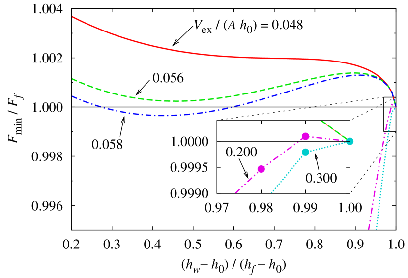
Figure 9: The minimal free energy $F_{\text{min}}(h_{w})=\min_{\alpha}F(\alpha,h_{w})$ as a function of the wetting film thickness $h_{w}$ for $A/(\pi h_{0}^{2})=100^{2}$, $\phi_{0}/\sigma=0.5$, and several values of $V_{\mathrm{ex}}/(A\,h_{0})$ ranging from $0.048$ to $0.3$. $F_{f}=A\,(\sigma+\phi(h_{f}))$ is the free energy of the corresponding flat film solution for these parameters. The morphological transition between flat films and nano-droplets occurs between $V_{\mathrm{ex}}/(A\,h_{0})=0.058$ and $0.056$. For $V_{\mathrm{ex}}/(A\,h_{0})>0.2$ the flat film solution appears to becomes unstable as expected from Eq. (18) (in the inset see the enlarged view of the region near $h_{w}=h_{f}$). The symbols indicate the points calculated numerically. For $V_{\mathrm{ex}}/(A\,h_{0})=0.3$ a small barrier cannot be ruled out on the basis of the available numerical data.

This morphological transition is visualized even better by forming vertical cuts of the free energy landscape at fixed $h_{w}$, i.e., parallel to the $\alpha$-axis and by seeking the minimum of the free energy $F$ within each cut as a function of $\alpha$. This renders $F_{\mathrm{min}}(h_{w})=\min_{\alpha}F(\alpha,h_{w})$. In Fig. 9 the corresponding the minimal free energy $F_{\mathrm{min}}(h_{w})$ is shown as a function of the wetting film thickness $h_{w}$. The energy scale is normalized by the free energy $F_{f}(V_{\mathrm{ex}})$ of the corresponding flat film solution (compare Figs. 4 to 8). For very small excess volumes the free energy as a function of the wetting film thickness is monotonically decreasing and the only minimum which occurs is the one corresponding to a flat film of thickness $h_{f}$ so that $(h_{w}-h_{0})/(h_{f}-h_{0})=1$. For intermediate excess volumes ($0.05\lesssim V_{\mathrm{ex}}/(A\,h_{0})\lesssim 0.058$ in Fig. 9) there is a second minimum corresponding to a metastable droplet. With increasing $V_{\mathrm{ex}}$ this droplet minimum deepens until it is as deep as the minimum corresponding to the flat film (at $V_{\mathrm{ex}}/(A\,h_{0})\approx 0.057$). This marks the point of the morphological transition between a flat film and a droplet solution. Increasing the excess volume even further the droplet solution becomes more stable. According to the inset of Fig. 9 it seems that the flat film solution (i.e., $(h_{w}-h_{0})/(h_{f}-h_{0})=1$) becomes unstable for $V_{\mathrm{ex}}/(A\,h_{0})\geq 0.2$ as expected from Eq. (18). However, for this latter value a tiny free energy barrier cannot be ruled out on the basis of the available numerical data.

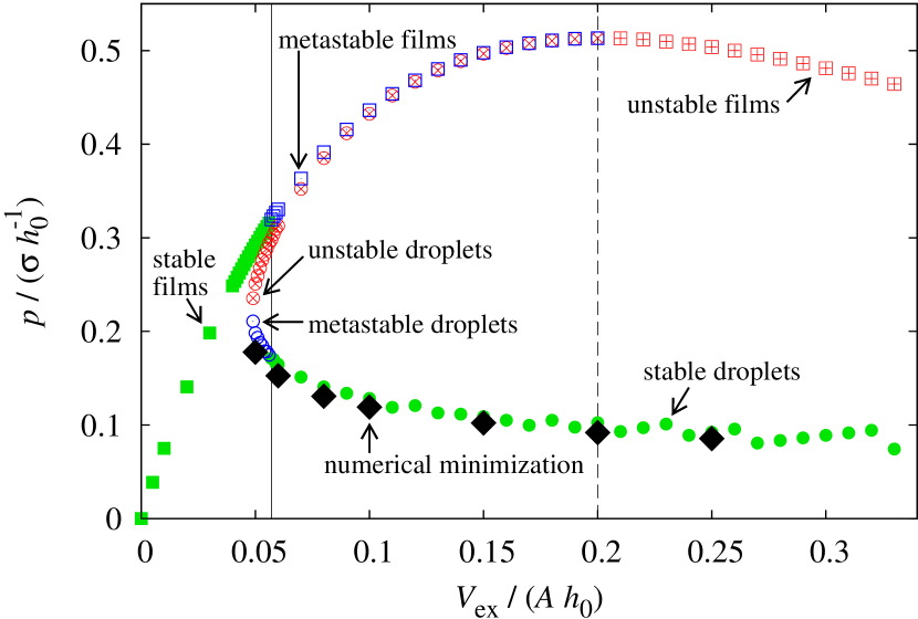
Figure 10: The pressure $p$ in units of $\sigma/h_{0}$ as a function of $V_{\mathrm{ex}}/(A\,h_{0})$ for a fixed substrate size, $A/(\pi\,h_{0}^{2})=100^{2}$, and $\phi_{0}/\sigma=0.5$ as obtained from the approximate free energy expression $F(\alpha,h_{w})$. Global minima (full green), local minima (open blue), and saddle points or local maxima (symbols with red crosses) are shown. The upper branch corresponds to flat films (boxes) and the lower one to nano-droplets (circles). Within the reduced model we have $p=-\Pi(h_{w}^{eq})$ (see Eq. (22)). The pressure values obtained from a numerical minimization of Eq. (3) (black diamonds; $p\approx-\Pi(h_{w}^{eq})$, see Eq. (20)) agree well with the results obtained from the approximate free energy. The dashed vertical line indicates the volume at which $h_{f}=h_{i}$. At this volume the unstable droplet branch merges with the flat film branch. The full vertical line indicates the morphological transition between the film and the droplet configurations.

Figure 10 shows the pressure $p$ as a function of the excess volume for a homogeneous film of thickness $h_{f}$ (upper curve) and for the droplet solution (lower curve). The upper branch is exact while the lower branch is calculated by minimizing the approximate expression for the free energy $F(\alpha,h_{w})$ defined in Eq. (21). According to Eq. (22), for both branches one has $p=-\Pi(h_{w}^{eq})$. Figure 10 also shows pressure values obtained by numerical minimization of the full functional $\mathcal{F}$ (for which, according to Eq. (20), $p\approx-\Pi(h_{w}^{eq})$). The pressure in the flat films (upper curve) is given by $p=-\Pi(h_{f})$ with $h_{f}/h_{0}=V_{\mathrm{ex}}/A+1$ (see Eq. (22)) and it has a maximum at $V_{\mathrm{ex}}/(A\,h_{0})=0.2$, corresponding to $h_{f}=h_{i}$. For excess volumes smaller than $V_{\mathrm{ex}}/(A\,h_{0})=0.2$ the flat film solution is metastable or stable. For larger excess volumes, the flat film solution is linearly unstable. However, the spinodal wavelength is extremely large close to the pressure maximum such that, according to Eq. (17) and for the given substrate size, the instability actually sets in only for $V_{\mathrm{ex}}/(A\,h_{0})>0.2011$. In Fig. 10 for $0.05<V_{\mathrm{ex}}/(A\,h_{0})<0.2$ there are two curves below the curve corresponding to the flat film solution; the upper one (red circles with crosses) corresponds to a saddle point in the free energy landscape and the lower one corresponds to a (potentially local) minimum. Both branches represent droplet solutions. The unstable branch ends at $V_{\mathrm{ex}}/(A\,h_{0})=0.2$, i.e., at the maximum of the pressure in the flat film solution. The three curves in Fig. 10 form a hysteresis loop. The value of $V_{\mathrm{ex}}/(A\,h_{0})$, at which the transition (thin vertical line in Fig. 10) between a flat film and a droplet occurs, can be obtained either by comparing free energies directly or via a Maxwell construction (see Fig. 11). The latter can be shown by integrating $p=\partial\mathcal{F}/\partial V=\partial\mathcal{F}/\partial V_{\mathrm{ex}}$ (due to Eq. (3) and since $dV/dV_{\mathrm{ex}}=1$ due to Eq. (12)) along $p(V)$: $\mathcal{F}(V)-\mathcal{F}(V_{0})=\int_{V_{0}}^{V}p(V)\,dV$. Starting the integration at the volume $V_{\text{eq}}$ at which the free energy of the film (upper branch) and the stable droplet (lowest branch) are equal (see Fig. 11) one integrates up to $V=V_{i}$, i.e., the volume of a film of thickness $h_{i}$ at which the unstable droplet branch merges with the film branch. The result, i.e., the sum of area (1) and (2) in Fig. 11, is the difference of the free energies of a film with volume $V_{i}$ and a film with volume $V_{\text{eq}}$. At $V_{i}$ one switches to the unstable droplet branch and integrates down to its end at $V_{m}$. The result is the difference between area (1) and the sum of area (3) and area (4). From there one continues on the metastable droplet branch up to $V_{\text{eq}}$, which adds area (4). As a result, the difference of the free energy of a flat film of volume $V_{\text{eq}}$ and a stable droplet of the same volume is the difference between area (1) and area (3). For the chosen model interface potential in Eq. (4) the flat film solution becomes linearly unstable at the value of $V_{\mathrm{ex}}/(A\,h_{0})$ (i.e., $0.2$ in Fig. 10), where the unstable droplet curve merges with the flat film curve.

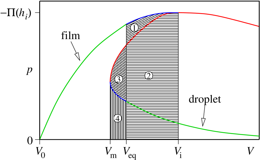
Figure 11: Sketch of the Maxwell construction leading to the position of the thin full vertical line in Fig. 10. The color code corresponds to the one in Fig. 10: green, blue, and red indicate stable, metastable, and unstable states, respectively. $V_{0}$ denotes the volume of a film of thickness $h_{0}$, $V_{m}$ is the minimal volume required to form a droplet, $V_{\text{eq}}$ is the volume at which the free energies of the flat film and of the stable droplet are equal. For $V\nearrow V_{i}$ the branch of metastable flat films turns into a branch of unstable flat films. There also the branch of unstable droplets merges into the flat film branch.

Figure 12: The droplet volume $V_{d}=V-A\,h_{w}$ as function of $V_{\mathrm{ex}}/(A\,h_{0})$ (i.e., as a function of $V=V_{\mathrm{ex}}+A\,h_{0}$) for $\phi_{0}/\sigma=0.5$ and (a) $A/(h_{0}^{2}\,\pi)=100^{2}$ and (b) $A/(h_{0}^{2}\,\pi)=1000^{2}$ as obtained from the approximate expression $F(\alpha,h_{w})$ for the free energy: for fixed $V=V_{\mathrm{ex}}+A\,h_{0}$ the free energy landscapes (see, e.g., Figs. 6–8) have been calculated and the wetting film thicknesses $h_{w}$ of the droplet solutions—if they exist—have been determined. The upper branch corresponds to the stable (green) or metastable (blue) droplet solution. For (a) this is the lower branch in Fig. 10. The points on the abscissa correspond to stable (green) or metastable (blue) flat film solutions. The comparison between (a) and (b) shows that the minimal droplet size $V_{d}^{c}$ (for which the unstable and the metastable droplet branches meet) increases upon increasing the substrate area while the corresponding excess volume $V_{\mathrm{ex}}^{c}$ in units of the substrate area decreases.

In Fig. 10 the excess volume is expressed in terms of the substrate area. In order to discuss whether the minimal droplet size is determined by the interface potential or by the substrate size, one could fix the excess volume $V_{\mathrm{ex}}$ (as a measure for the droplet size) and the substrate potential and vary the substrate size $A$. But the excess volume is defined as the fluid volume above the height $h_{0}$ (see Eq. (12)) and increasing the substrate area $A$ for fixed $V_{\mathrm{ex}}$ means effectively reducing the droplet size. The droplet volume $V_{d}=V-A\,h_{w}$ above the height of the wetting film $h_{w}$ is a more suitable measure for the droplet size. For this reason in Fig. 12 we plot the droplet volume $V_{d}$ as a function of the excess volume $V_{\mathrm{ex}}$ for two substrate sizes. The data are obtained in the following way: for each fixed value of $A$ and of $V_{\mathrm{ex}}$ (i.e., for fixed total volume $V=V_{\mathrm{ex}}+A\,h_{0}$) the interfacial free energies as shown in Figs. 6–8 are calculated. The position of local and global minima and of saddle points (corresponding to stable, metastable, and unstable droplet or flat film solutions) are determined numerically, in particular the wetting film thickness $h_{w}$ from which one can determine the droplet volume $V_{d}=V_{\mathrm{ex}}-A\,(h_{w}+h_{0})$. As in Fig. 10, for large $V_{\mathrm{ex}}$ there are three branches of solutions (flat film solutions with $V_{d}=0$, unstable droplet solutions, and metastable or stable droplet solutions). For small $V_{\mathrm{ex}}$ there are only flat film solutions. The size $V_{d}^{c}=V_{d}(V_{\mathrm{ex}}=V_{\mathrm{ex}}^{c})$ of the smallest metastable droplet (which is identical to the size of the largest unstable droplet) increases with the substrate area, as well as the value $V_{\mathrm{ex}}^{c}$ of the corresponding excess volume. However, $V_{\mathrm{ex}}^{c}/(A\,h_{0})$ decreases upon increasing $A$ (compare Figs. 12(a) and (b)). This means, that the thickness $h_{f}^{c}=V_{\mathrm{ex}}^{c}/A$ of the flat film solution corresponding to the minimal droplet also decreases upon an increase of the substrate area.

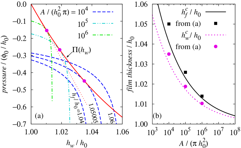
Figure 13: (a) Disjoining pressure $\Pi(h_{w})$ with $h_{0}<h_{w}<h_{f}$ (calculated for the model potential in Eq. (4)) in the wetting film (solid red line) and the right hand side of Eq. (27) with $R(h_{w},h_{f},A)$ from Eq. (29) (dashed blue lines) for $A/(\pi\,h_{0}^{2})=10^{4}$ and $\phi_{0}/\sigma=0.5$ as a function of the wetting film thickness $h_{w}$ for $h_{f}=1.04\,h_{0}$, $h_{f}=h_{f}^{c}=1.05005\,h_{0}$, and $h_{f}=1.06\,h_{0}$, which fixes $V=A\,h_{f}$ for a given $A$ (see Eq. (12)). We also show the right hand side of Eq. (27) for $A/(\pi\,h_{0}^{2})=10^{5}$ and $h_{f}=h_{f}^{c}=1.02587\,h_{0}$ (dash-double-dotted cyan line), as well as for $A/(\pi\,h_{0}^{2})=10^{6}$ and $h_{f}=h_{f}^{c}=1.01394\,h_{0}$ (dash-dotted green line). The thin dotted red line shows the linear fit to $\Pi(h_{w})$ at $h_{w}=h_{0}$. For $h_{f}=h_{f}^{c}(A)$ the curves $\Pi(h_{w})$ and the one for the right hand side of Eq. (27) touch each other at a single point at $h_{w}=h_{w}^{c}(A)$ indicated by a magenta circle. (b) $h_{f}^{c}$ and $h_{w}^{c}$ as a function of the substrate area $A$ in units of $\pi\,h_{0}^{2}$ as obtained graphically from (a) (black squares and magenta circles, respectively) and from the analytic approximation described in the main text (full black and dotted magenta line, respectively).

The nonexistence of droplet solutions for too small values of $V_{\mathrm{ex}}$ can be rationalized by considering a further simplified reduced expression for the free energy. Neglecting the influence of the disjoining pressure on the spherical cap the minimization problem for $F(\alpha,h_{w})$ yields (see Eq. (21) and up to the constant substrate-liquid surface tension)

$$F=(A-r^{2}\,\pi)\,\left[\sigma+\phi(h_{w})\right]+\sigma\,S_{d},$$ (24)

with $r=\sqrt{2\,h_{d}\,R-h_{d}^{2}}$ denoting the base radius of the drop (taken at $z=h_{w}$) and $S_{d}=2\,\pi\,R\,h_{d}$ denoting the surface area of a spherical cap of height $h_{d}$ and radius $R$. The volume of the spherical cap is given by $V_{d}=\frac{\pi}{3}\,h_{d}^{2}\,(3\,R-h_{d})$ and the total fluid volume by $V=V_{d}+A\,h_{w}$. It is convenient to write the volume constrained free energy

$$F(h_{d},h_{w})=\left[A\,\left(1+\frac{2\,h_{w}}{h_{d}}\right)-\frac{2\,V}{h_{d}}+\frac{\pi}{3}\,h_{d}^{2}\right]\,\phi(h_{w})\\ +\sigma\,\left(A+\pi\,h_{d}^{2}\right)$$ (25)

as a function of the droplet height $h_{d}$ rather than the droplet contact angle $\alpha$. The minimum of $F(h_{d},h_{w})$ follows from the zeroes of its first derivatives with respect to $h_{d}$ and $h_{w}$. Using the above expressions for $V$ and $V_{d}$ one obtains from $\partial F(h_{d},h_{w})/\partial h_{d}=0$

$$R\,\phi(h_{w})+\sigma\,h_{d}=0.$$ (26)

Using this expression together with the above expressions for $V$ and $V_{d}$ one obtains from $\partial F(h_{d},h_{w})/\partial h_{w}=0$, after reintroducing $\alpha$ via the geometric condition $r=R\,\sin\alpha$,

$$\Pi(h_{w})=-\frac{2\,\sigma}{R\,\left(1-\frac{\pi\,R^{2}\,\sin^{2}\alpha}{A}\right)}.$$ (27)

Apart from a small correction (which is small if $A$ is large compared with the base area $\pi\,R^{2}\,\sin^{2}\alpha$ of the droplet) Eq. (27) tells that the disjoining pressure in the film and the Laplace pressure $2\,\sigma\,H_{h}=-2\,\sigma/R$ (see Eq. (6)) in the droplet are equal (according to Eq. (7) both are equal to $p$). Using the geometric relation $\cos\alpha=1-h_{d}/R$ in Eq. (26) we also get

$$\cos\alpha=1+\frac{\phi(h_{w})}{\sigma}.$$ (28)

In the macroscopic limit $R\to\infty$ in Eq. (27) implies $\Pi(h_{w})\to 0$, i.e., $h_{w}\to h_{0}$ so that $\phi(h_{w})\to\phi(h_{0})=-\phi_{0}$ (see Fig. 1), and therefore $\alpha\to\theta_{\mathrm{eq}}$ (see Eq. (19)). As a function of $\alpha$, $R$, and $h_{w}$ the total conserved fluid volume is

$$V=A\,h_{w}+\frac{\pi\,R^{3}}{3}\,(2+\cos\alpha)\,(1-\cos\alpha)^{2}.$$ (29)

For a given value of $\alpha$ Eqs. (27) and (29) provide solutions for $h_{w}$ and $R$ only if $V$ is sufficiently large. The thickness $h_{w}$ can only vary between $h_{0}$ (i.e., the whole excess volume is concentrated in the droplet) and $h_{f}=V/A$ (i.e., there is no droplet). For $h_{w}=h_{0}$ the disjoining pressure $\Pi$ in the film is zero while the Laplace pressure $2\,\sigma\,H_{h}=-2\,\sigma/R$ in the droplet is negative. Both become more negative for increasing $h_{w}$ because the droplet shrinks and $\Pi^{\prime}(h_{0})<0$. The Laplace pressure diverges to $-\infty$ as $h_{w}\to h_{f}=V/A$ because the droplet volume $V_{d}$ (and therefore the droplet radius $R$) vanishes in this limit and $H_{h}=-1/R$. But the disjoining pressure is bound from below. With $\arccos[1+\phi(h_{w})/\sigma]$ (see Eq. (28)) Eq. (29) can be solved for $R$ yielding $R(h_{w},V,A)$ or

$$R(h_{w},h_{f},A)=\sqrt[3]{\frac{3\,A\,(h_{f}-h_{w})}{\pi\,\left[3+\frac{\phi(h_{w})}{\sigma}\right]\,\left[\frac{\phi(h_{w})}{\sigma}\right]^{2}}}$$ (30)

due to $V=A\,h_{f}$. Accordingly, one can consider both sides of Eq. (27) as a function of $h_{w}$ as shown in Fig. 13(a) where $\alpha$ is approximated by $\theta_{\mathrm{eq}}=\arccos(1-\phi_{0}/\sigma)$. The right hand side of Eq. (27) increases (decreases in absolute value) upon increasing $h_{f}/h_{0}=V/(A\,h_{0})$. For large $A/R^{2}$ and $h_{w}\approx h_{0}$, the right hand side of Eq. (27) is approximately given by

$$-\frac{\phi_{0}}{h_{0}}\,\frac{2}{\sqrt[3]{3}}\,\sqrt[3]{\frac{\frac{\sigma}{\phi_{0}}\,\left(3+\frac{\phi_{0}}{\sigma}\right)}{\frac{A}{\pi\,h_{0}^{2}}\,\frac{h_{f}-h_{w}}{h_{0}}}}.$$ (31)

The two curves only intersect if the fluid volume (or $h_{f}=V/A$) is sufficiently large (see the three blue dashed curves in Fig. 13(a)).

For sufficiently large excess volumes, i.e., for sufficiently large $h_{f}$ there are two intersections in Fig. 13(a). Because for fixed total volume $V$ increasing $h_{w}$ (i.e., increasing the amount of liquid in the film) means decreasing the droplet volume, the intersection at the larger values of $h_{w}$ corresponds to the unstable solution while the intersection at the smaller value of $h_{w}$ corresponds to the stable droplet solution. (The unstable droplet is always smaller than the stable one.) In the macroscopic limit $A/h_{0}^{2}\to\infty$ with fixed $h_{f}=h_{0}+V_{\mathrm{ex}}/A$ (see Eq. (23)) the stable solution moves to $h_{w}\to h_{0}$ . This means that the volume of the stable droplet gets very large because due to $h_{w}\to h_{0}$ the whole excess volume goes into the droplet. In the macroscopic limit, the unstable solution moves to $h_{w}\to h_{f}$. We can obtain the corresponding leading behavior by the following procedure. First we insert $R(h_{w},V,A)$ as obtained from Eq. (29) into Eq. (27) and we replace $\cos\alpha$ by the expression in Eq. (28). After substituting $V=A\,h_{f}$ we expand both sides in powers of $h_{w}-h_{f}$ and we obtain in leading order $h_{f}-h_{w}\sim 1/A$ . As a consequence, in the macroscopic limit the volume $V_{d}=A\,(h_{f}-h_{w})$ of the unstable droplet should converge to a finite value. However, this primitive model only applies to large droplet volumes and therefore this result for unstable drops might turn out to be an artefact of the approximations used.

As shown in Fig. 13(b) the critical average film thickness $h_{f}^{c}=V^{c}/A$ required for forming a droplet decreases as a function of the substrate area. For very large $A$ both $h_{f}^{c}$ and the corresponding wetting film thickness $h_{w}^{c}$ corresponding to the smallest possible droplet are very close to $h_{0}$ such that in Eq. (27) one can expand $\Pi(h_{w})$ around $h_{0}$ (see the thin dotted line in Fig. 13(a)). If one makes the additional approximations of using $\alpha\approx\theta_{\mathrm{eq}}$ and of reducing the right hand side of Eq. (27) to the Laplace pressure by neglecting the term $\sim A^{-1}$ in the denominator of the right hand side of Eq. (27), one can determine $h_{f}^{c}$ and $h_{w}^{c}$ analytically with the result $h_{f/w}^{c}-h_{0}\propto A^{-1/4}$ (see Fig. 13(b)). The drop volume is $V_{d}=V-A\,h_{w}=A\,(h_{f}-h_{w})$. Thus the volume of the smallest possible droplet diverges for $A\to\infty$ as $V_{d}^{c}=(h_{f}^{c}-h_{w}^{c})\,A\propto A^{3/4}$.

IV Summary and conclusions

We have studied the stability of nonvolatile flat films and droplets on smooth and chemically homogeneous substrates with finite surface area $A$. The analysis is based on density functional theory within the so-called sharp kink approximation, i.e., by minimizing the effective local interface Hamiltonian with the effective interface potential shown in Fig. 1.

The stability of flat films and of nano-droplets is strongly affected by finite size effects. We have shown that in these systems (i) spinodal dewetting can occur only if the substrate area $A$ is large enough to support the shortest unstable wavelength, (ii) there is a minimal size for droplets connected to a surrounding wetting layer, (iii) droplets are unstable with respect to drainage into a connected wetting films if the substrate area is too large, and (iv) that fluctuations of the droplet shape under the constraint of a fixed volume are more likely than volume fluctuations.

Our findings are manifestations of the general rule that long-wavelength instabilities are suppressed by finite size effects. The shortest instability wavelength $L_{c}=2\,\pi\,\sqrt{\sigma/|\phi^{\prime\prime}(h_{f})|}$ of spinodal dewetting depends on the material properties, i.e., on the surface tension $\sigma$ and on the effective interface potential $\phi(z)$, as well as on the average film thickness $h_{f}=V/A$, whereas $V$ is the conserved total liquid volume. In particular for film thicknesses close to inflection points of $\phi(z)$ and for thick films this wavelength becomes very large. For differentiable effective interface potentials the second derivative has a maximum (typically at a thickness of a few $h_{0}$ where $\phi^{\prime}(h_{0})=0$). Therefore the spinodal wavelength $L_{c}$ of films with the corresponding thickness has a minimum. Experimentally spinodal wavelengths of the order of microns have been reported seemann01b ; seemann01d . This means that spinodal dewetting can be suppressed by structuring the surface, e.g., by a periodic pattern of hydrophilic and hydrophobic stripes, the latter ones with a width smaller than $L_{c}$. The width of the hydrophilic stripes which is necessary to stabilize the film has to be determined separately.

We have calculated the shape of nano-droplets numerically as shown in Fig. 2 and we have determined the thickness $h_{w}$ of the wetting film on which the nano-droplet resides (see Table 1). Using a subset of trial function for the droplet shape which are parameterized by the contact angle of the droplet and by the wetting film thickness $h_{w}$ (see Fig. 3) we have mapped the free energy landscape of the system (see Figs. 4 and 6–9).

In contrast to macroscopic drops (see Fig. 4), for nano-droplets the influence of the wetting film to which they are connected cannot be neglected. If the excess volume $V_{\mathrm{ex}}=V-A\,h_{0}=(h_{f}-h_{0})\,A$ is fixed, there is a minimal substrate size below which no droplet solutions exist (see Fig. 5). Conversely, for a fixed substrate size $A$ one can find droplet solutions only above a critical (excess) volume (see Figs. 7 and 10). This is reminiscent of classical nucleation theory which also leads to the notion of a critical nucleus size. However, in the latter case one usually considers unbounded systems such that one cannot obtain stable droplet solutions at all. In the present case, the conserved total volume of fluid is distributed between a finite sized wetting film and a droplet; this allows for stable droplet solutions.

As illustrated in Fig. 11 the volume $V$ (or excess volume $V_{\mathrm{ex}}=V-A\,h_{0}$) at which the free energy of the flat film solution (a film of homogeneous thickness $h_{f}=V/A$) equals the free energy of the stable droplet (indicated by a thin vertical line in Fig. 10) can be determined by a Maxwell construction. This construction is based on the observation that the Lagrange multiplier $p$ (i.e., the pressure difference between the liquid and the vapor phase) is given by $p=\partial\mathcal{F}/\partial V$, i.e., by the partial derivative with respect to the chosen total volume $V$ (see Eq. (3)).

The size of the smallest possible droplet increases (see Fig. 12) and the thickness of the wetting film surrounding the droplet decreases upon increasing the substrate area (see Fig. 13). Within a suitable approximation of the free energy we have found that the volume $V_{d}^{c}$ of the smallest possible droplet diverges upon increasing the substrate size $A$ as $V_{d}^{c}/h_{0}^{3}\propto(A/h_{0}^{2})^{3/4}$. The proportionality factor depends on the equilibrium contact angle $\theta_{\mathrm{eq}}$ and for nonzero contact angles it is of the order of unity with $0.077$ as a lower bound (realized at $\theta_{\mathrm{eq}}=180^{\circ}$). For $h_{0}\approx 1\,\text{\AA}$ this means that the minimal droplet volume on substrates of size $A=1\,\mathrm{mm}^{2}$, $1\,\mu\mathrm{m}^{2}$, and $(100\,\mathrm{nm})^{2}$ equals that of a cube of edge length $300\,\mathrm{nm}$, $10\,\mathrm{nm}$, and $1.4\,\mathrm{nm}$, respectively. On the same substrate the volumes of the connected wetting films of thickness $1$ Å fit into cubes of an edge length of $4.6\,\mu\mathrm{m}$, $46\,\mathrm{nm}$, and $10\,\mathrm{nm}$, respectively, i.e., they are much larger. Our results show that nonetheless the finite extent of the substrate surface plays a significant role for the droplet formation and the associated morphological phase transition.

References

- (1) G. Reiter, Dewetting of highly elastic thin polymer films, Phys. Rev. Lett. 87, 186101 (4pp.) (2001).
- (2) R. Seemann, S. Herminghaus, and K. Jacobs, Gaining control of pattern formation of dewetting liquid films, J. Phys.: Condens. Matter 13, 4925–4938 (2001).
- (3) R. Seemann, S. Herminghaus, and K. Jacobs, Dewetting patterns and molecular forces: a reconciliation, Phys. Rev. Lett. 86, 5534–5537 (2001).
- (4) J. Becker, G. Grün, R. Seemann, H. Mantz, K. Jacobs, K. R. Mecke, and R. Blossey, Complex dewetting scenarios captured by thin film models, Nature Mat. 2, 59–63 (2003).
- (5) P. Müller-Buschbaum, Dewetting and pattern formation in thin polymer films as investigated in real and reciprocal space, J. Phys.: Condens. Matter 15, R1549–R1582 (2003).
- (6) R. Fetzer, K. Jacobs, A. Münch, B. Wagner, and T. P. Witelski, New slip regimes and the shape of dewetting thin liquid films, Phys. Rev. Lett. 95, 127801 (4pp.) (2005).
- (7) R. Fetzer, M. Rauscher, R. Seemann, K. Jacobs, and K. Mecke, Thermal noise influences fluid flow in thin films during spinodal dewetting, Phys. Rev. Lett. 99, 114503 (4pp.) (2007).
- (8) M. Hamieh, S. Al Akhrass, T. Hamieh, P. Damman, S. Gabriele, T. Vilmin, E. Raphaël, and G. Reiter, Influence of substrate properties on the dewetting dynamics of viscoelastic polymer films, J. Adhesion 83, 367–381 (2007).
- (9) J. Ralston, M. Popescu, and R. Sedev, Dynamics of wetting from an experimental point of view, Ann. Rev. Mater. Res. 38, 23–43 (2008).
- (10) R. Bausch, R. Blossey, and M. A. Burschka, Critical nuclei for wetting and dewetting, J. Phys. A: Math. Gen. 27, 1405–1406 (1994).
- (11) A. Bertozzi, G. Grün, and T. Witelski, Dewetting films: bifurcations and concentrations, Nonlinearity 14, 1569–1592 (2001).
- (12) U. Thiele, M. G. Velarde, and K. Neuffer, Dewetting: film rupture by nucleation in the spinodal regime, Phys. Rev. Lett. 87, 016104 (4pp.) (2001).
- (13) K. B. Glasner and T. P. Witelski, Coarsening dynamics of dewetting films, Phys. Rev. E 67, 016302 (12pp.) (2003).
- (14) R. Blossey, A. Münch, M. Rauscher, and B. Wagner, Slip vs. viscoelasticity in dewetting thin films, Eur. Phys. J. E 20, 267–271 (2006).
- (15) T. Vilmin and E. Raphaël, Dewetting of thin polymer films, Eur. Phys. J. E 21, 161–174 (2006).
- (16) E. Bertrand, T. D. Blake, V. Ledauphin, G. Ogonowski, J. De Coninck, D. Fornasiero, and J. Ralston, Dynamics of dewetting at the nanoscale using molecular dynamics, Langmuir 23, 3774–3785 (2007).
- (17) J. De Coninck and T. D. Blake, Wetting and molecular dynamics simulations of simple liquids, Ann. Rev. Mater. Res. 38, 1–22 (2008).
- (18) P. G. de Gennes, Wetting: statics and dynamics, Rev. Mod. Phys. 57, 827–860 (1985).
- (19) S. Dietrich, in Phase Transitions and Critical Phenomena, edited by C. Domb and J. L. Lebowitz (Academic, London, 1988), vol. 12, chap. 1, pp. 1–218.
- (20) M. Rauscher and S. Dietrich, Wetting phenomena in nanofluidics, Ann. Rev. Mater. Res. 38, 143–172 (2008).
- (21) M. Rauscher and S. Dietrich, in Handbook of Nanophysics, edited by K. D. Sattler (CRC, Boca Raton, 2010), vol. I: Principles and Methods, chap. 11, pp. 1–23.
- (22) R. J. Jackman, D. C. Duffy, E. Ostuni, N. D. Willmore, and G. M. Whitesides, Fabricating large arrays of microwells with arbitrary dimensions and filling them using discontinuous dewetting, Anal. Chem. 70, 2280–2287 (1998).
- (23) R. Lipowsky, P. Lenz, and P. Swain, Wetting and dewetting of structured and imprinted surfaces, Colloids Surf. A: Physicochem. Eng. Aspects 161, 3–22 (2000).
- (24) K. Kargupta and A. Sharma, Templating of thin films induced by dewetting on patterned surfaces, Phys. Rev. Lett. 86, 4536–4539 (2001).
- (25) K. Kargupta and A. Sharma, Creation of ordered patterns by dewetting of thin films on homogeneous and heterogeneous substrates, J. Colloid Interface Sci. 245, 99–115 (2002).
- (26) L. Brusch, H. Kühne, U. Thiele, and M. Bär, Dewetting of thin films on heterogeneous substrates: pinning versus coarsening, Phys. Rev. E 66, 011602 (5pp.) (2002).
- (27) U. Thiele, L. Brusch, M. Bestehorn, and M. Bär, Modelling thin film dewetting on structured surfaces and templates: bifurcation analysis and numerical simulations, Eur. Phys. J. E 11, 255–271 (2003).
- (28) S. Harkema, E. Schäffer, M. D. Morariu, and U. Steiner, Pattern replication by confined dewetting, Langmuir 19, 9714–9718 (2003).
- (29) A. Checco, B. M. Ocko, M. Tasinkevych, and S. Dietrich, Stability of thin wetting films on chemically nanostructured surfaces, Phys. Rev. Lett. 109, 166101 (5pp.) (2012).
- (30) S. Dietrich, M. N. Popescu, and M. Rauscher, Wetting on structured substrates, J. Phys.: Condens. Matter 17, S577-S593 (2005).
- (31) T. M. Squires and S. R. Quake, Microfluidics: fluid physics at the nanoliter scale, Rev. Mod. Phys. 77, 977–1026 (2005).
- (32) E. Delamarche, D. Juncker, and H. Schmid, Microfluidics for processing surfaces and miniaturizing biological assays, Adv. Mater. 17, 2911–2933 (2005).
- (33) J. Koplik, T. S. Lo, M. Rauscher, and S. Dietrich, Pearling instability of nanoscale fluid flow confined to a chemical channel, Phys. Fluids 18, 032104 (14 pp.) (2006).
- (34) M. Rauscher, S. Dietrich, and J. Koplik, Shear flow pumping in open microfluidic systems, Phys. Rev. Lett. 98, 224504 (4pp.) (2007).
- (35) S. Mechkov, M. Rauscher, and S. Dietrich, Stability of liquid ridges on chemical micro- and nanostripes, Phys. Rev. E 77, 061605 (10pp.) (2008).
- (36) F. Dutka, M. Napiórkowski, and S. Dietrich, Mesoscopic analysis of Gibbs’ criterion for sessile nanodroplets on trapezoidal substrates, J. Chem. Phys. 136, 064702 (20pp.) (2012).
- (37) M. A. Burschka, R. Blossey, and R. Bausch, Macroscopic shape of critical droplets in first-order wetting transitions, J. Phys. A: Math. Gen. 26, L1125–L1129 (1993).
- (38) S. Dietrich and M. Napiórkowski, Microscopic derivation of the effective interface Hamiltonian for liquid-vapor interfaces, Physica A 177, 437–442 (1991).
- (39) S. Dietrich and M. Napiórkowski, Analytic results for wetting transitions in the presence of van der Waals tails, Phys. Rev. A 43, 1861–1885 (1991).
- (40) M. Napiórkowski, W. Koch, and S. Dietrich, Wedge wetting by van der Waals fluids, Phys. Rev. A 45, 5760–5770 (1992).
- (41) J. S. Rowlinson and B. Widom, Molecular theory of capillarity (Dover, Mineola, 2002).
- (42) S. A. Safran, Statistical Thermodynamics of Surfaces, Interfaces, and Membranes, vol. 90 of Frontiers in physics (Westview, Boulder, 2003).
- (43) P.-G. de Gennes, F. Brochard-Wyart, and D. Quéré, Capillarity and wetting phenomena: drops, bubbles, pearls, waves (Springer, New York, 2004).
- (44) M. Napiórkowski and S. Dietrich, Structure of the effective Hamiltonian for liquid-vapor interfaces, Phys. Rev. E 47, 1836–1849 (1993).
- (45) J. O. Indekeu, Line tension near the wetting transition: results from an interface displacement model, Physica A 183, 439–461 (1992).
- (46) H. T. Dobbs and J. O. Indekeu, Line tension at wetting: interface displacement model beyond the gradient-squared approximation, Physica A 201, 457–481 (1993).
- (47) J. O. Indekeu, Line tension at wetting, Int. J. Mod. Phys. B 8, 309–345 (1994).
- (48) T. Getta and S. Dietrich, Line tension between fluid phases and a substrate, Phys. Rev. E 57, 655–671 (1998).
- (49) C. Bauer and S. Dietrich, Quantitative study of laterally inhomogeneous wetting films, Eur. Phys. J. B 10, 767–779 (1999).
- (50) C. Bauer and S. Dietrich, Shapes, contact angles, and line tensions of droplets on cylinders, Phys. Rev. E 62, 2428-2438 (2000).
- (51) L. Schimmele, M. Napiórkowski, and S. Dietrich, Conceptual aspects of line tensions, J. Chem. Phys. 127, 164715 (28pp.) (2007).
- (52) R. Evans, The nature of the liquid-vapour interface and other topics in the statistical mechanics of non-uniform, classical fluids, Adv. Phys. 28, 143–200 (1979).
- (53) K. Brakke, The surface evolver, Experimental Mathematics 1, 141–165 (1992).
- (54) A. Moosavi, M. Rauscher, and S. Dietrich, Motion of nanodroplets near edges and wedges, Phys. Rev. Lett. 97, 236101 (4pp.) (2006).
- (55) A. Moosavi, M. Rauscher, and S. Dietrich, Dynamics of nanodroplets on topographically structured substrates, J. Phys.: Condens. Matter 21, 464120 (24pp.) (2009).
- (56) T. Young, An essay on the cohesion of fluids, Philos. Trans. Roy. Soc. London 95, 65–87 (1805).
- (57) Note1, this calculation can be significantly simplified by approximating (which is independent of ) and by neglecting the term in the denominator of the right hand side of Eq. (27).