Characterization of phase-averaged coherent states

Abstract

We present the full characterization of phase-randomized or phase-averaged coherent states, a class of states exploited in communication channels and in decoy state-based quantum key distribution protocols. In particular, we report on the suitable formalism to analytically describe the main features of this class of states and on their experimental investigation, that results in agreement with theory. We also show the results we obtained by manipulating the phase-averaged coherent states with linear optical elements and testify their good quality by employing some non-Gaussianity measures and the concept of mutual information.

1 Introduction

Laser radiation, which can be described in terms of coherent states, plays a relevant role in practical communication schemes. One of the main advantages of coherent states over more exotic quantum states, such as squeezed ones, is that they can propagate over long distances, only suffering attenuation and without altering their fundamental properties. A coherent state is characterized by a Poissonian photon-number statistics and a well-defined optical phase. Thus, one can easily implement phase-shifted keyed communication in which the logical information (the bit) is encoded in two coherent states with the same amplitude and a $\pi$-difference in phase. Nevertheless, this kind of communication channel lacks security. Remarkably, very recently quantum key distribution involving coherent states and decoy states has been realized and it has been pointed out that phase-averaged coherent states may enhance the security of the channel [1, 2, 3]. In this case, the high degree of accuracy in the phase randomization process is one of the main requirements.

By contrast to coherent states, which are described by Gaussian Wigner functions, phase-averaged coherent states clearly exhibit non-Gaussian features [4]. Thus, the systematic study of the nature of these states and the possibility to manipulate them can be considered of real interest in enhancing the performances of the communication protocols in which they are employed [5].

In this paper we investigate the main features of phase-averaged coherent states and report on their fully experimental characterization by addressing the measurement of the photon-number statistics and the reconstruction of the Wigner function. Furthermore, we perform basic manipulation experiments by means of linear optical elements, in order to assess the usefulness of these states for communication and information processing. The detection of such states is performed in the mesoscopic photon-number regime by means of hybrid photodetectors.

The plan of the paper is as follows. In section 2 we recall several properties of phase-averaged coherent states like photon-number statistics and purity. We also present the experimental scheme used for the generation, characterization and manipulation of such states. Section 3 is devoted to their basic description using the characteristic functions and the corresponding quasiprobability densities. In this section we also report on the strategy and realization of the experimental reconstruction of the Wigner function. Non-Gaussianity of the phase-averaged coherent states and its experimental measurement are addressed in section 4. Section 5 investigates the linear operations with phase-averaged coherent states performed by a beam splitter. Here we give a complete analytic description of the output one-mode reduced states. These superpositions turn out to be Fock-diagonal and are interesting for quantum information processing. We find a good agreement between theory and our experimental results for what concerns non-Gaussianity and mutual information of the beam-splitter output states. Our concluding remarks are drawn in section 6.

2 Quantum description of phase-averaged coherent states

A single-mode phase-randomized or phase-averaged coherent state (PHAV) is obtained by randomizing the phase $\phi$ of a coherent state:

$$|\beta\rangle=\exp{\left(-\frac{1}{2}|\beta|^{2}\right)}\sum_{n=0}^{\infty}\frac{|\beta|^{n}\,e^{in\phi}}{\sqrt{n!}}|n\rangle,$$ (1)

with $\beta=|\beta|\,e^{i\phi}$. Any PHAV $\hat{\varrho}$ is diagonal in the photon-number basis, namely:

$$\hat{\varrho}=\int_{0}^{2\pi}\frac{d\phi}{2\pi}\,|\beta\rangle\langle\beta|=\sum_{n=0}^{\infty}\varrho_{nn}|n\rangle\langle n|,$$ (2)

where

$$\varrho_{nn}=\exp{\left(-|\beta|^{2}\right)}\frac{|\beta|^{2n}}{n!},$$ (3)

is a Poissonian distribution. Therefore, randomizing the phase of a coherent state does not change its photon-number distribution [see (3)]. Moreover, due to the diagonal structure of its density matrix, the statistical properties of a PHAV can be fully described by the photon-number distribution. Indeed, while $|\beta\rangle$ is a pure state, the degree of purity $\mu[\hat{\varrho}]$ of the PHAV $\hat{\varrho}$ can be directly evaluated by the photon-number distribution and is given by:

$$\mu[\hat{\varrho}]=\sum_{n=0}^{\infty}\varrho_{nn}^{2}=\exp{\left(-2|\beta|^{2}\right)}\,I_{0}(2|\beta|^{2}),$$ (4)

where $I_{0}(z)$ is the modified zeroth-order Bessel function of the first kind. The purity $\mu[\hat{\varrho}]$ is a strictly decreasing function of the mean number of photons $\langle\hat{a}^{{\dagger}}\hat{a}\rangle={\rm Tr}[\hat{\varrho}\,\hat{a}^{{\dagger}}\hat{a}]=|\beta|^{2}$ ($\hat{a}$ is the annihilation operator and $[\hat{a},\hat{a}^{{\dagger}}]=\hat{\mathbbm{I}}$).

From the experimental point of view, we obtained this class of states by sending the second-harmonics pulses of a mode-locked Nd:YLF laser amplified at 500 Hz (High-Q Laser Production) to a mirror mounted on a piezo-electric movement (see figure 1). The displacement of the piezoelectric movement, which is controlled by a function generator, is operated at a frequency of 100 Hz and covers a 12 $\mu$m span [6].

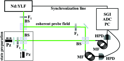
Figure 1: Experimental setup. F_j: variable neutral density filter; BS: 50:50 beam splitter; Pz: piezoelectric movement; MF: multimode fiber (600 $\mu$m core); HPD: hybrid photodetector.

In figure 2 we show the detected photon distributions of three PHAVs at different energy values, obtained by using a direct detection scheme employing a hybrid photodetector (HPD, R10467U-40, maximum quantum efficiency $\sim$ 0.5 at 500 nm, Hamamatsu) characterized by a partial photon-counting capability and a linear response up to 100 photons [7, 8]. In the same figure, we also show the corresponding theoretical photon-number statistics for detected photons [the photocount distribution is simply obtained by using (3) and replacing $|\beta|^{2}$ by $M\equiv\eta|\beta|^{2}$, where $\eta$ is the overall quantum efficiency].

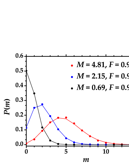
Figure 2: Detected-photon distribution of PHAV state for three different mean values. Coloured dots: experimental data, lines: theoretical expectations. The purity is $\mu[\hat{\varrho}]=0.13$ (red plot), $\mu[\hat{\varrho}]=0.20$ (blue plot) and $\mu[\hat{\varrho}]=0.39$ (black plot).

The good agreement between experimental data and theory can be quantified by calculating the fidelity (see $F$ values reported in figure 2): $F=\sum_{m=0}^{\bar{m}}\sqrt{P_{\rm th}(m)P(m)}$, in which $P_{\rm th}(m)$ and $P(m)$ are the theoretical and experimental distributions, respectively, and the sum is extended up to the maximum detected-photon number $\bar{m}$ above which both $P_{\rm th}(m)$ and $P(m)$ become negligible.

3 Basic characterization

We insert (2) into the well-known definition of the characteristic functions (CFs):

$$\chi({\lambda;s})\equiv\exp{\left(\frac{s}{2}|\lambda|^{2}\right)}\,{\rm Tr}[\hat{\varrho}\hat{D}(\lambda)],\quad(-1\leq s\leq 1)$$ (5)

to write:

$$\chi(\lambda;s)=\exp{\left(-\frac{1-s}{2}|\lambda|^{2}\right)}\,\sum_{n=0}^{\infty}\varrho_{nn}\,L_{n}\left(|\lambda|^{2}\right).$$ (6)

The series (6) is obtained by substitution of the diagonal matrix elements of the displacement operator $\hat{D}(\lambda)=\exp(\lambda\hat{a}^{\dagger}-\lambda^{*}\hat{a})$ in the photon-number basis, namely:

$$\langle n|\hat{D}(\lambda)|n\rangle=\exp\left(-\frac{1}{2}|\lambda|^{2}\right)\,L_{n}\left(|\lambda|^{2}\right),$$ (7)

where $L_{n}(z)$ is a Laguerre polynomial. By using the generating function of the Laguerre polynomials [9, 10]:

$$\sum_{n=0}^{\infty}L_{n}(z)\frac{x^{n}}{n!}={\rm e}^{x}J_{0}\left(2\sqrt{xz}\right)$$ (8)

where $J_{0}(z)$ is a Bessel function of the first kind, we get:

$$\chi(\lambda;s)=\exp{\left(-\frac{1-s}{2}|\lambda|^{2}\right)}\,J_{0}(2|\beta||\lambda|).$$ (9)

The Fourier transform of the CFs in (9) gives us the set of quasiprobability densities [11, 12]:

$$W(z;s)=\frac{1}{\pi}\int_{\mathbbm{C}}{\rm d}^{2}{\lambda}\;\exp{(z\lambda^{*}-z^{*}\lambda)}\,\chi(\lambda;s),$$ (10)

which explicitly read [9, 10]:

$$W(z;s)=\frac{2}{1-s}\exp{\left[-\frac{2}{1-s}\left(|\beta|^{2}+|z|^{2}\right)\right]}\,I_{0}\!\left(\frac{4|z||\beta|}{1-s}\right).$$ (11)

If we set $s=-1$ in (11), we obtain the $Q$ function:

$$Q(z) = \frac{1}{\pi}W(z;-1)$$ (12)

$$= \frac{1}{\pi}\exp{\left[-\left(|\beta|^{2}+|z|^{2}\right)\right]}\,I_{0}\left(2|z||\beta|\right).$$

The $P$ function retrieved for $s=1$ by employing asymptotic expansions of Bessel functions is expressed in terms of Dirac’s $\delta$ distribution:

$$P(z) = W(z;1)$$ (13)

$$= \frac{1}{\pi}\delta\left(|z|^{2}-|\beta|^{2}\right)=\frac{1}{2\pi|\beta|}\delta\left(|z|-|\beta|\right),$$

and the last equality follows from the properties of the $\delta$ distribution. Equation (13) shows us that the mixed state obtained by averaging over the phase of a pure coherent state preserves the important feature of being at the classicality threshold (remember that the coherent states are the only pure states at the classicality threshold).

Finally, for $s=0$ we get the Wigner function:

$$W(z)=2\exp{\left[-2\left(|\beta|^{2}+|z|^{2}\right)\right]}I_{0}\left(4|z||\beta|\right).$$ (14)

which is positive everywhere in the phase space. Recently, states with positive Wigner functions have become interesting for efficient classical simulation of a broad class of quantum optics experiments. In [13, 14] a protocol for classical simulations using non-Gaussian states with positive Wigner function was presented (see also the more recent [15]). Note that the Wigner function in (14) is not Gaussian, a feature that becomes evident from the plot of the function that shows a dip at the origin of the phase space (see figure 3).

In order to experimentally reconstruct the Wigner function of PHAVs we adopted the same strategy presented in [16] and based on the measurements of the statistics of the state under investigation mixed at a beam splitter (BS) with a coherent probe field whose amplitude and phase can be continuously changed [17, 18, 19]. As the PHAV is a diagonal state, its Wigner function is phase insensitive, $i.e.$ it exhibits a rotational invariance about the origin of the phase space.

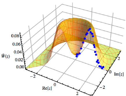
Figure 3: Experimental reconstruction of a section of the Wigner function of a PHAV with $|\beta|^{2}=1.97$ and $\xi=0.999$. Blue dots: experimental data, orange mesh: theoretical expectation.

For this reason, in figure 3 we show the experimental data (blue dots) corresponding to a section of the Wigner function superimposed to the theoretical surface (orange mesh):

$$\tilde{W}\left(\sqrt{\xi}\alpha\right)=W\left(\sqrt{\xi}\alpha\right)\exp\left[-(|\alpha|+|\beta|)\sqrt{1-\xi}\right],$$ (15)

$\xi$ being the overall (spatial and temporal) overlap between the probe field and PHAV [16]. In (15), $|\beta|^{2}$ is now the mean number of photons we measured, which includes the quantum efficiency. In fact, it is worth noting that for classical states the functional form of the Wigner function is preserved also in the presence of losses and its expression, given in terms of detected photons, reads $\tilde{W}(\alpha)=\frac{2}{\pi}\sum_{m=0}^{\infty}(-1)^{m}p_{m,\alpha}^{\ el}$, where $p_{m,\alpha}^{\ el}$ represent the detected-photon-number distributions of the state to be measured displaced by the probe field [16].

4 Non-Gaussianity of PHAVs

In order to quantify the non-Gaussanity of PHAVs, here we compare three different measures of non-Gaussianity recently introduced [20, 21, 22, 23] and completely determined by the density matrix in (2) and (3). All the three measures compare the properties of the state under investigation $\hat{\varrho}$ with that of a Gaussian reference state, $\hat{\sigma}$, having the same mean value and covariance matrix as $\hat{\varrho}$. In the case of PHAVs, the reference Gaussian state is a thermal state with mean occupancy $|\beta|^{2}$.

The first measure is based on the Hilbert-Schmidt distance:

$$\varepsilon_{\rm A}[\hat{\varrho}]=\frac{D^{2}_{\rm HS}[\hat{\varrho},\hat{\sigma}]}{\mu[\hat{\varrho}]}=\frac{\mu[\hat{\varrho}]+\mu[\hat{\sigma}]-2\kappa[\hat{\varrho},\hat{\sigma}]}{2\mu[\hat{\varrho}]},$$ (16)

where $\mu$ is the purity of the state and $\kappa[\hat{\varrho},\hat{\sigma}]=$Tr$[\hat{\varrho}\hat{\sigma}]$ [20]. The Hilbert-Schmidt distance can be analytically calculated by using the purity (4), the degree of purity of the reference thermal state $\mu[\hat{\sigma}]=(2|\beta|^{2}+1)^{-1}$ and the expression of $\kappa[\hat{\varrho},\hat{\sigma}]$:

$$\kappa[\hat{\varrho},\hat{\sigma}]=\frac{1}{|\beta|^{2}+1}\exp{\left(-\frac{|\beta|^{2}}{|\beta|^{2}+1}\right)}.$$ (17)

The second measure is the relative entropy of non-Gaussianity defined as:

$$\varepsilon_{\rm B}[\hat{\varrho}]=S(\hat{\sigma})-S(\hat{\varrho}),$$ (18)

where $S(\hat{\varrho})=-\hbox{Tr}[\hat{\varrho}\ln\hat{\varrho}]$ is the von Neumann entropy of the state $\hat{\varrho}$ [21]. For all diagonal states, we have $S(\hat{\varrho})=-\sum_{n}\varrho_{nn}\ln\varrho_{nn}$, where in the present case $\varrho_{nn}$ is given in (3), and $S(\hat{\sigma})=\left(|\beta|^{2}+1\right)\ln\left(|\beta|^{2}+1\right)-|\beta|^{2}\ln|\beta|^{2}$.

The last measure we study has been recently introduced in [23] and is based on the quantum fidelity, namely:

$$\varepsilon_{\rm C}[\hat{\varrho}]=1-\sqrt{{\cal F}(\hat{\varrho},\hat{\sigma})},$$ (19)

where:

$${\cal F}(\hat{\varrho},\hat{\sigma})=\left\{{\rm Tr}\left[\sqrt{\sqrt{\hat{\varrho}}\,\hat{\sigma}\,\sqrt{\hat{\varrho}}}\right]\right\}^{2}$$ (20)

is the Uhlmann fidelity [24]. This measure can readily be evaluated for Fock-diagonal states since they commute with their reference thermal states.

It is worth noting that the evaluation of the considered measures only requires quantities that can be experimentally accessed by direct detection, as they can be expressed in terms of photon-number distributions [26].

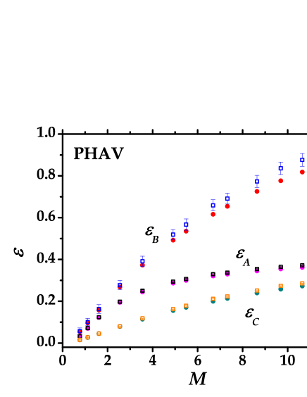
Figure 4: Comparison between the three measures of non-Gaussianity in the case of PHAVs as functions of the mean number of photons. Open squared symbols: experimental data, dots: theoretical expectations.

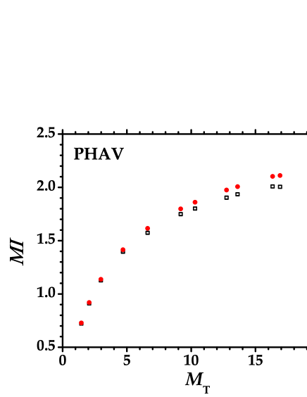
Figure 5: Mutual information between the two outputs of the BS at which a PHAV with energy $M_{\rm T}$ is divided. Open squared symbols: experimental data, red dots: theory. The error bars are smaller than the symbol size.

Figure 4 shows the behaviour of the three non-Gaussianity measures as functions of the average number $M$ of detected photons in the case of PHAVs. It is evident that the behaviours of the three measures are very similar to each other except for the absolute values [27].

5 Advanced characterization and manipulation

When a coherent state $|\beta\rangle$ is mixed with the vacuum at a BS with transmissivity $\tau$, the two emerging beams are excited in the product state $|\sqrt{\tau}\beta\rangle\otimes|\sqrt{1-\tau}\beta\rangle$ and thus are uncorrelated. Nevertheless, when we consider a PHAV as the input state, a correlation arises at the two outputs, even if intensity correlations still vanish [28]. The total amount of correlation of the output bipartite state $\hat{\varrho}_{12}$ can be evaluated in terms of the mutual information ($MI$):

$$MI(\hat{\varrho}_{12})=S(\hat{\varrho}_{1})+S(\hat{\varrho}_{2})-S(\hat{\varrho}_{12}),$$ (21)

where $\hat{\varrho}_{k}={\rm Tr}_{h}[\hat{\varrho}_{12}]$ ($h,k=1,2$ and $k\neq h$) are the output reduced states and $S(\hat{\varrho})$ is the von Neumann entropy. In figure 5 we plot the experimental data (open squared symbols) and the theoretical predictions (red dots) of the $MI$ as a function of the energy of the input PHAV. We experimentally measured this parameter by using a scheme involving two hybrid photodetectors to simultaneously detect the light at the two outputs of the BS [29], as shown in figure 1. Since from the experimental point of view it is not possible to measure both the input and output states simultaneously, in order to assess the last term in (21) we assumed that the input state was a PHAV with energy equal to the sum of the two output channels (losses at the BS are negligible). We also notice that in figure 5 the slight discrepancy between experiment and theory appearing at increasing values of the input energy can be due to some saturation effect of the acquisition chain.

We have also investigated another interesting state obtained by the interference of two PHAVs (see figure 1): we will refer to this state, which is still diagonal in the photon-number basis, as 2-PHAV [26]. The 2-PHAV can find useful applications in passive decoy state quantum key distribution [5]. To describe the 2-PHAV state, we start observing that when two uncorrelated field modes described by a product CF $\chi_{0}(\lambda_{1},\lambda_{2};s)=\chi_{01}(\lambda_{1};s)\,\chi_{02}(\lambda_{2};s)$ are mixed at a BS with transmissivity $\tau$, the output two-mode CF may be written as follows $\chi(\lambda_{1},\lambda_{2};s)=\chi_{01}(\zeta_{1};s)\,\chi_{02}(\zeta_{2};s)$ with $\zeta_{1}=\lambda_{1}\sqrt{\tau}-\lambda_{2}\sqrt{1-\tau},\;\;\zeta_{2}=\lambda_{2}\sqrt{\tau}+\lambda_{1}\sqrt{1-\tau}$ [4]. Therefore, the CF of the 2-PHAV state, obtained by taking only one of the output modes, can be formally written as (the CF of the other mode can be obtained by replacing $\tau$ with $1-\tau$):

$$\chi(\lambda;s)=\chi_{01}\left(\lambda\sqrt{\tau};s\right)\,\chi_{02}\left(\lambda\sqrt{1-\tau};s\right),$$ (22)

which follows from the partial-trace rule in the reciprocal phase space. (22) gives the following multiplication rule for the input states of the type (9):

$$\chi(\lambda;s)=\exp{\left(-\frac{1-s}{2}|\lambda|^{2}\right)}J_{0}\left(2|\beta_{1}||\lambda|\sqrt{\tau}\right)J_{0}\left(2|\beta_{2}||\lambda|\sqrt{1-\tau}\right),$$ (23)

$\beta_{1}$ and $\beta_{2}$ are the coherent amplitudes of the corresponding interfering PHAVs. Note that $\chi(\lambda;s)\equiv\chi(|\lambda|;s)$, as expected for phase-insensitive states.

In order to obtain the photon statistics of the 2-PHAV, we can follow two strategies. On the one hand, we can use the expansion of the density operator in terms of displacement operators [11]:

$$\hat{\varrho}=\frac{1}{\pi}\int_{\mathbbm{C}}{\rm d}^{2}\lambda\,\chi(\lambda;0)\,\hat{D}(-\lambda).$$ (24)

Therefore, the matrix elements of a phase-insensitive single-mode state described by the CF $\chi(|\lambda|)\equiv\chi(\lambda;0)$ may be written as:

$$\varrho_{lm}=2\;\delta_{lm}\int_{0}^{\infty}{\rm d}|\lambda|\,|\lambda|\exp{\left(-\frac{1}{2}|\lambda|^{2}\right)}\,\chi(|\lambda|)\,L_{m}\left(|\lambda|^{2}\right),$$ (25)

where we used (7) and performed the integration over the polar angle, thus being left with an integral over $|\lambda|$.

On the other hand, we can exploit high-order correlation functions via the series [11, 12]:

$$\varrho_{nn}=\frac{1}{n!}\sum_{k=0}^{\infty}\frac{(-1)^{k-n}}{(k-n)!}\langle(\hat{a}^{{\dagger}})^{k}\hat{a}^{k}\rangle.$$ (26)

Using a generating-function method, we are able to derive the $k$th-order correlation functions in terms of Legendre polynomials $P_{k}(x)$:

$$\langle(\hat{a}^{{\dagger}})^{k}\hat{a}^{k}\rangle=\left[|\beta_{1}|^{2}\tau+|\beta_{2}|^{2}(1-\tau)\right]^{k}\,u^{k}\,P_{k}\left(\frac{1}{u}\right),$$ (27)

where $u$ is the ratio:

$$u=\frac{\big{|}|\beta_{1}|^{2}\tau-|\beta_{2}|^{2}(1-\tau)\big{|}}{|\beta_{1}|^{2}\tau+|\beta_{2}|^{2}(1-\tau)}.$$ (28)

The $k$th-order normalized correlation functions are then:

$$g^{(k)}(0)=\frac{\langle(\hat{a}^{{\dagger}})^{k}\hat{a}^{k}\rangle}{\langle\hat{a}^{{\dagger}}\hat{a}\rangle^{k}}=u^{k}P_{k}\left(\frac{1}{u}\right).$$ (29)

Now, thanks to the relationship (26) we obtain the density matrix elements as series expansions involving Legendre polynomials:

$$\varrho_{nn}=\,\frac{1}{n!}\sum_{k=0}^{\infty}\frac{(-1)^{k-n}}{(k-n)!}\left[|\beta_{1}|^{2}\tau+|\beta_{2}|^{2}(1-\tau)\right]^{k}\,u^{k}\,P_{k}\left(\frac{1}{u}\right).$$ (30)

In particular, if $\tau=1/2$ (balanced BS) and $|\beta_{1}|=|\beta_{2}|=|\beta|$ (identical inputs), we find a simple result for the degree of coherence (29), namely:

$$g^{(k)}(0)=\frac{(2k-1)!!}{k!}>1,\qquad(k>1),$$ (31)

which indicates a super-Poissonian photon statistics. The photon-number distribution is obtained after some algebra via (26) as:

$$\varrho_{nn}=\,\frac{(2n-1)!!}{(n!)^{2}}\,|\beta|^{2n}\,\exp{\left(-2|\beta|^{2}\right)}\,{{}_{1}F_{1}}\left(\frac{1}{2};n+1;2|\beta|^{2}\right),$$ (32)

where ${{}_{1}F_{1}}(q;p;z)$ is a confluent hypergeometric function [9, 30].

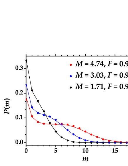
Figure 6: ”Detected-photon distribution of a balanced 2-PHAV state for three different mean values. Coloured dots: experimental data, lines: theoretical expectations (32). The purity is $\mu[\hat{\varrho}]=0.09$ (red plot), $\mu[\hat{\varrho}]=0.13$ (blue plot) and $\mu[\hat{\varrho}]=0.21$ (black plot).

In figure 6 we have plotted the photon-number distribution (32) for different energy values (coloured lines). We remark the good agreement between experimental data (coloured dots) and theory predictions confirmed also by the high values of the fidelity.

Finally, we have obtained the set of quasiprobability densities associated with a 2-PHAV as having the following expansion:

$$W(\alpha;s)=\,2\exp{\left(-\frac{2|\alpha|^{2}}{1-s}\right)}$$

$$\times\sum_{k=0}^{\infty}\frac{(-1)^{k}}{k!}\left(\frac{2(|\beta_{1}|^{2}T+|\beta_{2}|^{2}R)}{1-s}\right)^{k}u^{k}\,P_{k}\left(\frac{1}{u}\right)L_{k}\left(\frac{2|\alpha|^{2}}{1-s}\right),$$ (33)

where $P_{k}(z)$ are Legendre polynomials and $u$ is defined in (28). In particular, the quasiprobability densities of the balanced state (32) have a simpler form due to the explicit correlation functions (31). We get:

$$W(\alpha;s)=\,2\exp{\left(-\frac{2|\alpha|^{2}}{1-s}\right)}\sum_{k=0}^{\infty}\frac{(2k-1)!!}{(k!)^{2}}\left(-\frac{2|\beta|^{2}}{1-s}\right)^{k}L_{k}\left(\frac{2|\alpha|^{2}}{1-s}\right).$$ (34)

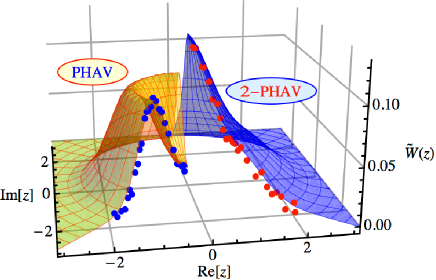
Figure 7: Left: Experimental reconstruction of a section of the Wigner function of a PHAV with $|\beta|^{2}=1.97$ and $\xi=0.999$. Blue dots: experimental data, orange mesh: theoretical expectation. Right: Experimental reconstruction of a section of the Wigner function of a balanced 2-PHAV with $|\beta_{1}|^{2}=1.03$, $|\beta_{2}|^{2}=0.91$, $\xi_{\rm P}=0.95$ and $\xi_{\rm S}=1$. Red dots: experimental data, blue mesh: theoretical expectation.

In figure 7 we report a section of the phase-insensitive Wigner function of a 2-PHAV (on the right) obtained by the interference at a balanced BS of two identical PHAVs (whose section of Wigner function is shown on the left). Even in the case of 2-PHAV, the experimental data (red dots) are well superimposed to the theoretical surface (blue mesh):

$$\tilde{W}_{\rm 2-PHAV}(\sqrt{\xi_{\rm P}}\alpha)=\,W_{\rm 2-PHAV}(\sqrt{\xi}_{\rm P}\alpha)\exp\Big{[}-|\alpha|\sqrt{1-\xi_{\rm P}}-(|\beta_{1}|+|\beta_{2}|)\sqrt{1-\xi_{\rm S}}\Big{]},$$ (35)

where $\xi_{\rm P}$ describes the overall overlap between the probe and the 2-PHAV and $\xi_{\rm S}$ the overall overlap between the two components of the 2-PHAV. It is evident that the single PHAV has a dip at the origin of the phase space, whereas the 2-PHAV has a peak. This difference results in a reduction of non-Gaussianity of the 2-PHAV with respect to that of a single PHAV at fixed energy, as testified by the non-Gaussianity measures introduced above [26, 27]. To stress this result, in figure 8 we show the behaviour of the three measures as functions of the energy values $M$ for a balanced 2-PHAV: we can notice that the absolute values of $\varepsilon_{k}$, $k=A,B,C$ are smaller than the ones we obtained in the case of a single PHAV. Moreover, in figure 9 we plot the same measures as functions of the balancing between the two components of the 2-PHAV at fixed energy value $M$. As one may expect, the three measures monotonically decrease at increasing the balancing. In fact, the most unbalanced condition reduces to the case in which there is only a single PHAV, whereas the most balanced one corresponds to have a balanced 2-PHAV.

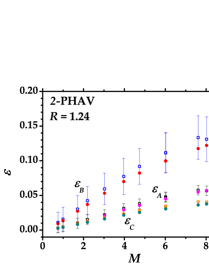
Figure 8: Comparison between the three measures of non-Gaussianity in the case of balanced 2-PHAVs as functions of the mean number of photons. Open squared symbols: experimental data, dots: theoretical expectations.

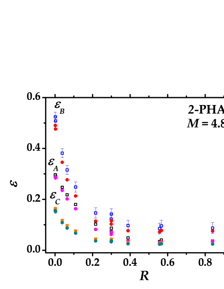
Figure 9: Comparison between the three measures of non-Gaussianity in the case of 2-PHAVs at fixed total energy as functions of the balancing between the two single PHAVs. Open squared symbols: experimental data, dots: theoretical expectations.

As in the case of a single PHAV, when a 2-PHAV state is mixed with the vacuum at a 50:50 BS, the two outputs show a correlated nature, testified by the non-zero value of the mutual information. In figure 10 we report the $MI$ between the two outputs of the BS at which a balanced 2-PHAV is divided as a function of the input energy value. Furthermore, figure 11 shows the $MI$ at fixed input energy of the 2-PHAV as a function of the ratio $R=|\beta_{1}|/|\beta_{2}|$ between the two single PHAVs used to generate the 2-PHAV state.

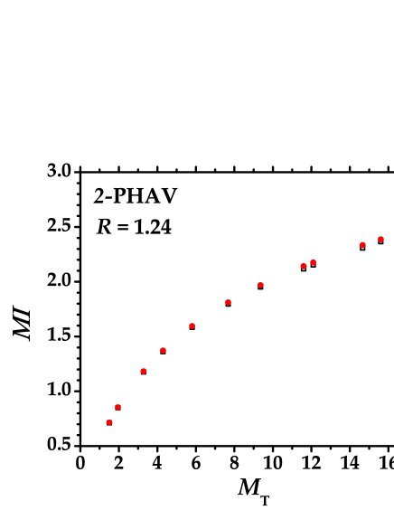
Figure 10: Mutual information between the two outputs of the BS at which a balanced 2-PHAV is divided as a function of the total input energy $M_{T}$. Open squared symbols: experimental data, red dots: theory. The error bars are smaller than the symbol size.

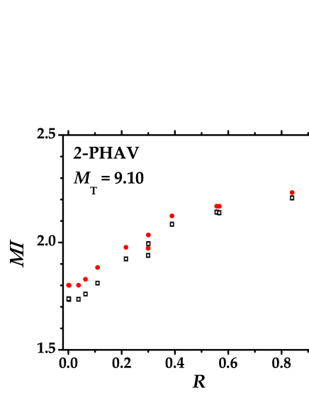
Figure 11: Mutual information between the two outputs of the BS at which a 2-PHAV at fixed input energy $M_{T}$ is divided as a function of the ratio $R=|\beta_{1}|/|\beta_{2}|$ between the energies of the two PHAVs generating the 2-PHAV state. Open squared symbols: experimental data, red dots: theory. The error bars are smaller than the symbol size.

In both figures the accordance between the experimental data (open squared symbols), whose error bars are smaller than the symbol size, and the theoretical predictions (red dots) is good. As in the case of a single PHAV, in order to assess the last term in (21) we again assumed that the input state was a 2-PHAV with energy equal to the sum of the two output channels.

6 Concluding remarks

In conclusion, we have studied the main properties of PHAVs: we have developed an analytic description and verified the theoretical predictions by means of a direct detection scheme involving hybrid photodetectors. In detail, we have investigated the detected photon-number distribution and the Wigner function that is non-Gaussian. Moreover, we have used three different non-Gaussianity measures, all based on quantities experimentally accessed by direct detection, to quantify the non-Gaussianity amount and have proven the consistency of the different approaches. Furthermore, we have manipulated PHAVs by means of linear optical elements and generated a new class of phase-randomized states, namely 2-PHAVs, obtained as superpositions of two PHAVs at a BS. The consistent experimental and theoretical results we have obtained in the characterization of both PHAVs and their superpositions 2-PHAVs reinforce the possibility of using them for applications to communication protocols. These classical states appear to be robust, experimentally accessible and theoretically convenient. The investigation of the non-Gaussianity and correlations of some other output BS-states manipulated by conditional measurements is one of our present interests.

References

References

- [1] Lo H-K, Ma X and Chen K 2005 Phys. Rev. Lett.94 230504
- [2] Zhao Y, Qi B and Lo H-K 2007 Appl. Phys. Lett. 90 044106
- [3] Inamori H, Ltkenhaus N and Mayers D 2007 Eur. Phys. J. D 41 599
- [4] Olivares S Eur. Phys. J. Special Topics 2012 203 3
- [5] Curty M, Moroder T, Ma X and Lütkenhaus N 2009 Opt. Lett. 34 3238
- [6] Bondani M, Allevi A and Andreoni A 2009 Adv. Sci. Lett. 2 463
- [7] Bondani M, Allevi A, Agliati A and Andreoni A 2009 J. Mod. Opt. 56 226
- [8] Andreoni A and Bondani M 2009 Phys. Rev. A 80 013819
- [9] Erdélyi A, Magnus W, Oberhettinger F and Tricomi F G 1953 Higher Transcendental Functions (New York, McGraw–Hill, vol 1 and 2)
- [10] Watson G N 1944 A treatise on the theory of Bessel functions (Cambridge University Press, Second edition)
- [11] Cahill K E and Glauber R J 1969 Phys. Rev. 177 1857
- [12] Cahill K E and Glauber R J 1969 Phys. Rev. 177 1882
- [13] Veitch V, Ferrie C, Gross D and Emerson J 2012 New J. Phys. 14 113011
- [14] Veitch V, Wiebe N, Ferrie C and Emerson J 2012 Efficient simulation scheme for a class of quantum optics experiments with non-negative Wigner representation Preprint arXiv:1210.1783 [quant-ph]
- [15] Mari A and Eisert J 2012 Phys. Rev. Lett.109 230503
- [16] Bondani M, Allevi A and Andreoni A 2009 Opt. Lett. 34 1444
- [17] Wallentowitz S and Vogel W 1996 Phys. Rev. A 53 4528
- [18] Banaszek K and Wdkiewicz K 1996 Phys. Rev. Lett.76 4344
- [19] Allevi A, Andreoni A, Bondani A, Brida G, Genovese M, Gramegna M, Olivares S, Paris M G A, Traina P and Zambra G 2009 Phys. Rev A 80 022114
- [20] Genoni M G, Paris M G A and Banaszek K 2007 Phys. Rev. A 76 042327
- [21] Genoni M G, Paris M G A and Banaszek K 2007 Phys. Rev. A 78 060303(R)
- [22] Genoni M G and Paris M G Phys. Rev. A 2010 82 052341.
- [23] Ghiu I, Marian P and Marian T A 2010 Measures of non-Gaussianity for one-mode field states Preprint arXiv:1210.1929 [quant-ph]
- [24] Uhlmann A 1976 Rep. Math. Phys. 9 273
- [25] Uhlmann A 1986 Rep. Math. Phys. 24 229
- [26] Allevi A, Olivares S and Bondani M 2012 Opt. Express 20 24850
- [27] Allevi A, Olivares S and Bondani M 2012 Int. J. Quantum Inf. 10 1241006
- [28] This results follows from the form of the joint photon statistics of the two outgoing modes that is factorized and reads , where is the Poisson distribution.
- [29] Allevi A, Bondani M and Andreoni A 2012 Opt. Lett. 35 1707
- [30] Zambra G, Allevi A, Bondani M, Andreoni A and Paris M G A 2007 Int. J. Quantum Inf. 5 305