Agreement of Neutrino Deep Inelastic Scattering Data with Global Fits of Parton Distributions

Abstract

The compatibility of neutrino-nucleus deep inelastic scattering data within the universal, factorizable nuclear parton distribution functions has been studied independently by several groups in the past few years. The conclusions are contradictory, ranging from a violation of the universality up to a good agreement, most of the controversy originating from the use of the neutrino-nucleus data from the NuTeV Collaboration. Here, we pay attention to non-negligible differences in the absolute normalization between different neutrino data sets. We find that such variations are large enough to prevent a tensionless fit to all data simultaneously and could therefore misleadingly point towards nonuniversal nuclear effects. We propose a concrete method to deal with the absolute normalization and show that an agreement between independent neutrino data sets is established.

A well-established procedure in nearly all phenomenological analyses of high-energy collisions involving hadrons is the division of the cross sections in universal sets of parton distribution functions (PDFs) $f_{i}(x,Q^{2})$ and short distance partonic processes. Here, $x$ is the momentum variable, $i$ labels the parton types, and $Q^{2}$ is the scale specific for the process. A theoretical foundation for such a procedure is provided by the theorem of collinear factorization Collins:1989gx , applicable to a wide range of hard (involving a large scale $Q^{2}>1\,{\rm GeV}^{2}$) processes in high-energy lepton+nucleon and nucleon+nucleon collisions. Although the non perturbative nature of the PDFs still prevents their precise calculation from the first principles of QCD, their scale dependence is given by the well-known Dokshitzer-Gribov-Lipatov-Altrarelli-Parisi (DGLAP) equations Dokshitzer:sg ; Gribov:ri ; Gribov:rt ; Altarelli:1977zs which resum the large logarithms $\sim\log(Q^{2})$ emerging from collinear QCD radiation. Ultimately, the validity of the factorization is verified in global analyses comparing a diverse set of experimental cross sections to the PDF-dependent calculated values. The initial conditions $f_{i}(x,Q_{0}^{2})$ for the DGLAP evolution are iteratively adjusted to see if a single set that can reproduce all the data exists. The PDFs and their uncertainties extracted in this way provide an indispensable tool for estimating signals, backgrounds and acceptances in other high-energy experiments. Clearly, the validity of factorization is of utmost importance for the phenomenology of high-energy hadronic collisions.

The global analyses of the nuclear parton distribution functions (nPDFs) study the applicability of the collinear factorization in hard processes involving bound nucleons. The most recent analyses Eskola:2009uj ; Hirai:2007sx ; Schienbein:2009kk ; deFlorian:2011fp include data on charged lepton nuclear deep inelastic scattering (DIS); Drell-Yan dilepton production in proton-nucleus collisions; and, in some cases, production of high transverse momentum pions in deuteron-gold collisions and neutrino-nucleus DIS. The good overall agreement with the available high-energy data supports the existence of universal, process-independent nPDFs. The nPDFs find applications in high-energy nucleus-nucleus collisions, playing an essential role e.g. in the heavy-ion program of the LHC.

The adequacy of the factorization in nuclear environment is of importance also from the point of view of free nucleon analyses Martin:2009iq ; Ball:2011uy ; Nadolsky:2008zw , which often wish to employ nuclear data as an additional constraint. One such process is the neutrino-nucleus DIS, which is useful for constraining e.g. the strange quark distribution, but the weakness of the neutrino interactions requires the use of a nuclear target. This process has recently invoked special attention as its compatibility within the framework of universal nPDFs was questioned Schienbein:2009kk ; Schienbein:2007fs . It was even declared Kovarik:2010uv that there is no way to satisfactorily reproduce the neutrino-nucleus and the other nuclear data simultaneously with a single set of nPDFs. This could have far-reaching consequences as the inability to find a set of nPDFs which at the same time describes all the considered data is the expected sign e.g. of a violation of the universality, or a breakdown of the DGLAP evolution. However, the same signal can also occur if one or more of the experimental data sets contains unrecognized systematic inaccuracies.

Contradictory results were first presented in Paukkunen:2010hb , where up-to-date nPDFs were found to give an excellent overall agreement with neutrino data from CDHSW Berge:1989hr , CHORUS Onengut:2005kv and NuTeV Tzanov:2005kr Collaborations, although issues with the normalization of the NuTeV data were identified possibly explaining the results of Kovarik:2010uv . Similar conclusions were reached in deFlorian:2011fp where data from all these experiments were utilized in a global nPDF analysis without an apparent disagreement. However, the baseline PDFs utilized there Martin:2009iq were already constrained by the NuTeV DIS data and their uncertainties were treated as additional, uncorrelated point-to-point errors. Furthermore, the analysis did not use the absolute cross sections, but the far more scarce structure function data. Given all this, the neutrino data did not carry as heavy an importance as in Kovarik:2010uv . For more comprehensive review of the present situation, see Kopeliovich:2012kw .

In this Letter, we will show that when accounting for the overall normalization of the experimental data in neutrino DIS, all three data sets do show a uniform pattern of nuclear modifications, well reproduced by the existing nPDFs. This reinforces the conclusions of Paukkunen:2010hb , in a model-independent way, supporting the functionality of the factorization in neutrino DIS. We make the point even more concrete by employing a method based on the Hessian error analysis to verify the consistency of these data with CTEQ6.6 Nadolsky:2008zw and EPS09 Eskola:2009uj global fits.

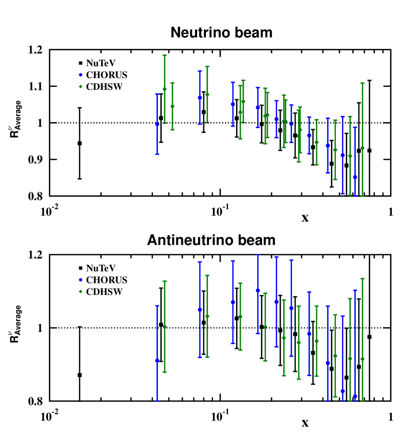
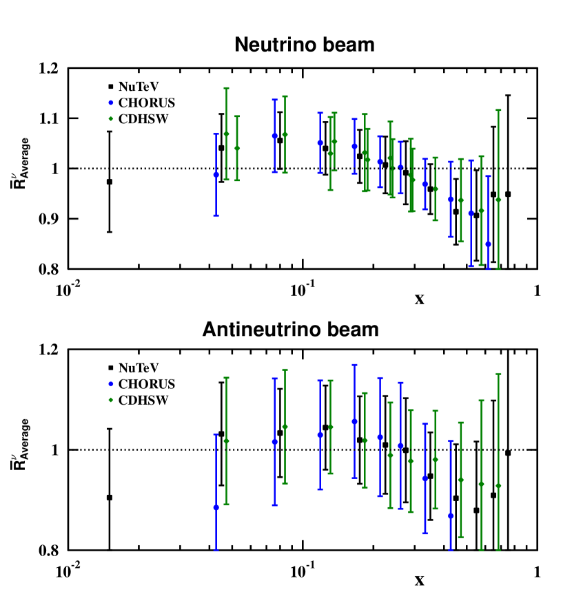
Figure 1: The neutrino and antineutrino data presented as $R^{\nu}_{\rm Average}$ (left-hand panels), and as $\overline{R}^{\nu}_{\rm Average}$ (right-hand panels). The CHORUS (blue circles) and CDHSW (green diamonds) data have been horizontally shifted from the NuTeV (black squares) data points for clarity.

We utilize the neutrino-nucleus DIS data from the NuTeV Tzanov:2005kr , CHORUS Onengut:2005kv and CDHSW Berge:1989hr experiments. The difficulty in dealing with the neutrino data is that no reference data from hydrogen or deuterium target are available and we are forced to use the absolute experimental cross sections $\sigma^{\nu}_{\rm exp}$ instead of cross section ratios. However, in order to better see the nuclear effects we still prefer to present the data as ratios

$$R^{\rm\nu}(x,y,E)\equiv\frac{\sigma^{\nu}_{\rm exp}(x,y,E)}{\sigma^{\nu}_{\rm CTEQ6.6}(x,y,E)},$$ (1)

where the theoretical cross sections ${\sigma^{\nu}_{\rm CTEQ6.6}}$ are calculated with the CTEQ6.6M central set. As in Paukkunen:2010hb , the theoretical calculations include corrections for the target mass and electroweak radiation, and are carried out in the SACOT-prescription Kramer:2000hn of the variable flavor number scheme. In order to avoid higher-twist effects we restrict the virtuality $Q^{2}$ and the final state invariant mass $W$ by conditions $Q_{\rm cut}^{2}>4\,{\rm GeV}^{2}$, and $W_{\rm cut}^{2}>12.25\,{\rm GeV}^{2}$. This leaves us with 2136 NuTeV, 824 CHORUS, and 937 CDHSW data points. For a concise presentation of this large amount of data, we form an average

$$R^{\nu}_{\rm Average}(x)\equiv\left(\sum^{N}_{i\in{\rm fixed}\,x}\frac{R_{i}^{\nu}}{\delta_{i}}\right)\left(\sum^{N}_{i\in{\rm fixed}\,x}\frac{1}{\delta_{i}}\right)^{-1}\pm N\times\left(\sum^{N}_{i\in{\rm fixed}\,x}\frac{1}{\delta_{i}}\right)^{-1},$$ (2)

where $\delta_{i}$ is the experimental error (statistical and systematic added in quadrature), and the sum runs over all data points in the same $x$ bin. This procedure neatly summarizes the main features of the neutrino data as a function of $x$, but we stress that it is used here only for plotting the data, the numerical results being computed using the absolute cross sections. The ratios constructed this way are shown in the left-hand panels of Figure 1. Although the data from different experiments appear to be in rough mutual agreement, the scatter is still non-negligible. In particular, the NuTeV neutrino data seem to lie systematically below the rest and as such are likely to trigger tension in a global fit — especially so if the NuTeV correlated systematic errors are taken seriously as in Kovarik:2010uv . However, as a function of $x$ the shape of the data seems to follow the usual nuclear effect, suggesting that the problem is rather in the absolute normalization, as already conjectured in Paukkunen:2010hb . For this reason, we define

$$I_{\rm exp}^{\nu}(E)\equiv\sum_{i\in{\rm fixed}\,E}\sigma_{{\rm exp},i}(x,y,E)\times B_{i}(x,y),$$ (3)

and similarly for the theoretical calculation. The factor $B_{i}(x,y)$ represents the size of the experimental $(x,y)$ bin making $I_{\rm exp}^{\nu}(E)$ thereby an estimate for the integrated cross section. Now, instead of Eq. (1) we consider the ratio of the normalized cross sections

$$\overline{R}^{\rm\nu}(x,y,E)\equiv\frac{\sigma^{\nu}_{\rm exp}(x,y,E)/I^{\nu}_{\rm exp}(E)}{\sigma^{\nu}_{\rm CTEQ6.6}(x,y,E)/I^{\nu}_{\rm CTEQ6.6}(E)}.$$ (4)

The averaged neutrino and antineutrino data normalized in this way are plotted in the right-hand panels of Figure 1, demonstrating how all the considered data seem to fall in agreement. In particular, the NuTeV neutrino data have moved upwards while the CHORUS and CDHSW neutrino data have remained essentially unchanged. This observation suggests that the origin of the difficulties in accommodating the neutrino data in a global fit Kovarik:2010uv is due to an unnoticed problem in the experimental normalization of the NuTeV data — that the uncertainties have probably been underestimated by the experiment.

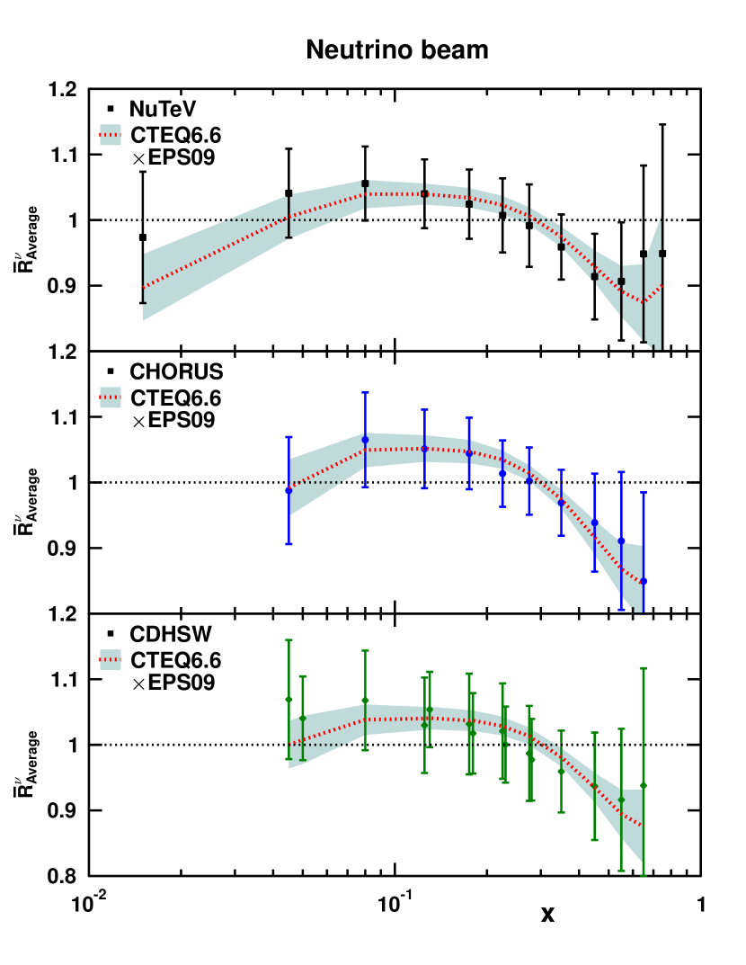
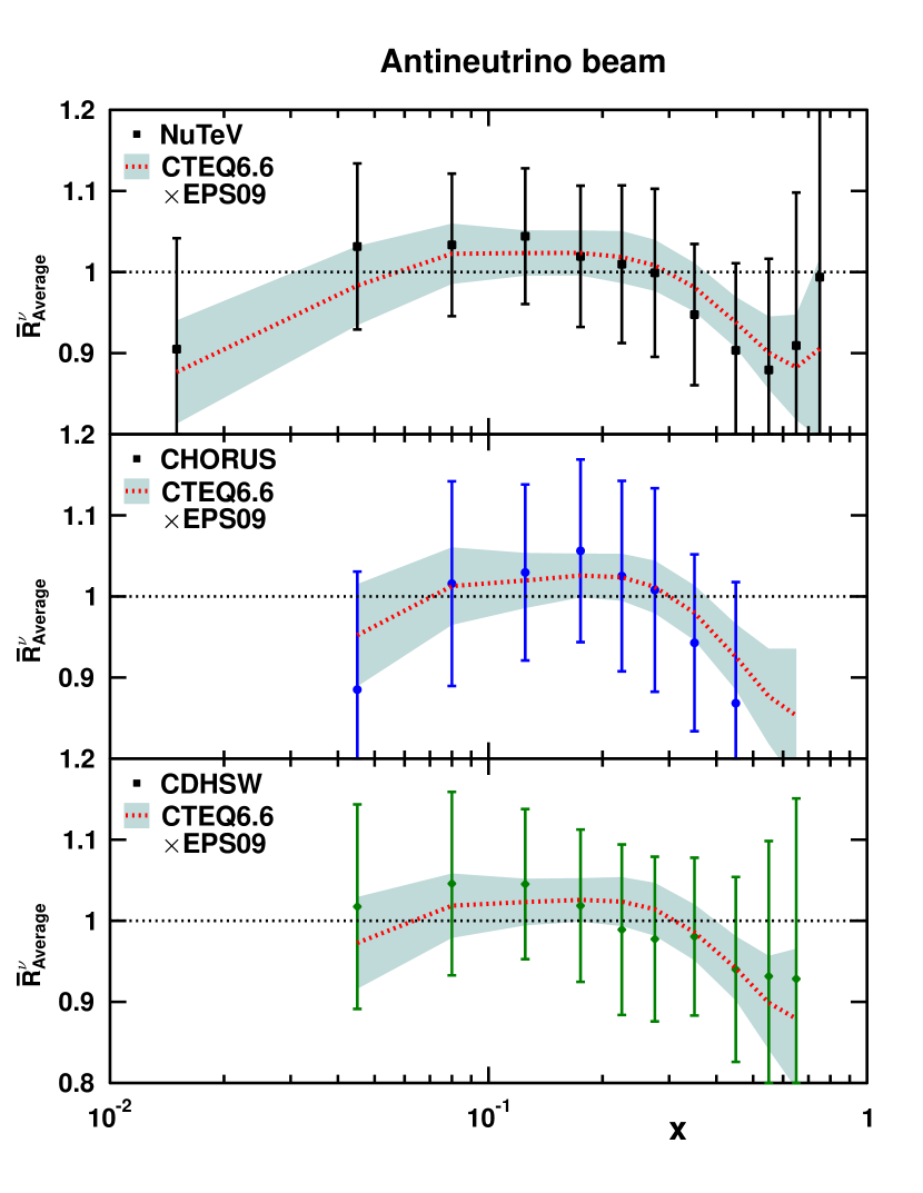
Figure 2: The experimental $\overline{R}^{\nu}_{\rm Average}$ compared to the predictions from CTEQ6.6 and EPS09.

In order to see how the normalized data compare with the predictions from the present nuclear PDFs, we replace in Eq. (4) the experimental cross sections by the theoretical ones computed with the bound proton PDFs $f_{i}^{A}(x,Q^{2})$ obtained standardly by

$$f_{i}^{A}(x,Q^{2})\equiv R_{i}^{A,{\rm EPS09}}(x,Q^{2})f_{i}^{\rm CTEQ6.6M}(x,Q^{2}),$$ (5)

where the factor $R_{i}^{A,{\rm EPS09}}$ represents the EPS09 Eskola:2009uj nuclear modification in free proton PDF $f_{i}^{\rm CTEQ6.6M}(x,Q^{2})$. The results are shown in Figure 2, where the data points are the same as in the right-hand panels of Figure 1, and the band indicates the theoretical calculations with all PDF uncertainties added in quadrature Eskola:2009uj . The good agreement indicates that it should be possible to include these data in global fits without significant mutual disagreement or tension with the other data sets. We note that in the normalization procedure described here, also part of the PDF uncertainties cancel thereby making the theoretical predictions more solid.

We turn now to a more quantitative description of the data sets accounting for the normalization. The technique described here is based on the Hessian uncertainty analysis Pumplin:2001ct performed e.g. in the EPS09 and CTEQ6.6 global fits . The neighborhood of the minimum $\chi^{2}$ is approximated by an expansion

$$\chi^{2}\approx\chi^{2}_{0}+\sum_{ij}\delta a_{i}H_{ij}\delta a_{j}=\chi^{2}_{0}+\sum_{i}z_{i}^{2},$$ (6)

where $\delta a_{j}$ is the deviation of the fit parameter $a_{j}$ from its best-fit value. By diagonalizing the Hessian matrix $H_{ij}$ one finds the uncorrelated parameter directions $z_{j}$ in terms of which the central set $S_{0}$, and the error sets $S_{k}^{\pm}$ are defined:

$$z(S_{0}) = \left(0,0,...,0\right)$$

$$z(S^{\pm}_{1}) = \pm\sqrt{\Delta\chi^{2}}\left(1,0,...,0\right)$$ (7)

$$z(S^{\pm}_{2}) = \pm\sqrt{\Delta\chi^{2}}\left(0,1,...,0\right)$$

$$\vdots$$

where $\Delta\chi^{2}$ is the maximum permitted deviation from the minimum $\chi^{2}$. These sets enable the calculation of any PDF-dependent quantity $X$ at the origin and at the corners of the $z$ space, but in order to obtain an estimate in an arbitrary point $z(S)=(z_{1},z_{2},\ldots)$ close to the origin, we need to use a linear approximation

$$X\left[S\right]\approx X\left[S_{0}\right]+\sum_{k}\frac{\partial X\left[S\right]}{\partial z_{k}}{\Big{|}_{S=S_{0}}}z_{k}\approx X_{0}+{\bf D}\cdot{\bf w},$$ (8)

where

$$D_{k} \equiv \frac{X\left[S_{k}^{+}\right]-X\left[S_{k}^{-}\right]}{2}$$ (9)

$$w_{k} \equiv \frac{z_{k}}{\sqrt{\Delta\chi^{2}}}.$$ (10)

Let us now consider a larger data set $\{X^{\rm data}\}$. The agreement with the PDF set $S$ can be quantified by formally adding its $\chi^{2}$ contribution $\chi^{2}\{{X^{\rm data}}\}$ to Eq. (6)

$$\chi^{2}=\chi^{2}_{0}+\sum_{\{X^{\rm data}\}}\left[\frac{X_{k}\left[S\right]-X_{k}^{\rm data}}{\delta_{k}^{\rm data}}\right]^{2}+\Delta\chi^{2}\sum_{k}w_{k}^{2},$$ (11)

where $\delta_{k}^{\rm data}$ is again the experimental uncertainty and each $X_{k}\left[S\right]$ is given by Eq. (8). The weight vector ${\bf w}$ that minimizes the above $\chi^{2}$ is given by ${\bf w}_{\rm min}=-{\bf B}^{-1}{\bf a}$, where

$$B_{ij} = \sum_{k}\frac{D^{k}_{i}D^{k}_{j}}{\left(\delta_{k}^{\rm data}\right)^{2}}+\Delta\chi^{2}\delta_{ij}$$ (12)

$$a_{i} = \sum_{k}\frac{D_{i}^{k}\left(X_{k}\left[S_{0}\right]-X_{k}^{\rm data}\right)}{\left(\delta_{k}^{\rm data}\right)^{2}}$$ (13)

$$D_{l}^{k} = \frac{X_{k}\left[S_{l}^{+}\right]-X_{k}\left[S_{l}^{-}\right]}{2}.$$ (14)

The level of agreement between the data set $\{X^{\rm data}\}$ and the given set of PDFs is now quantified — not only by $\chi^{2}\{{X^{\rm data}}\}$ — but also by the length of the weight vector ${\bf w}_{\rm min}$. If $|{\bf w_{\rm min}}|<1$ the new data set could be included to the original fit within the confidence criterion determined in the analysis. That is, the “penalty term” $\Delta\chi^{2}\sum_{k}w_{k}^{2}$ in Eq. (11) remains below the acceptable value $\Delta\chi^{2}$. On the other hand, if $|{\bf w}_{\rm min}|>1$, notable tension between the new and the old data is bound to exist.

	All CTEQ6.6 and EPS09 error sets				Only EPS09 error sets
NuTeV	$\chi^{2}_{w=0}/N$	$\chi_{w_{\rm min}}^{2}/N$	EPS09-penalty	CTEQ-penalty	$\chi_{w_{\rm min}}^{2}/N$	EPS09-penalty
Normalization	0.84	0.77	13.9	35.4	0.81	33.8
No normalization	1.04	0.90	40.3	42.5	0.94	77.4
CHORUS	$\chi^{2}_{w=0}/N$	$\chi_{w_{\rm min}}^{2}/N$	EPS09-penalty	CTEQ-penalty	$\chi_{w_{\rm min}}^{2}/N$	EPS09-penalty
Normalization	0.70	0.69	2.13	2.63	0.70	2.48
No normalization	0.86	0.81	3.35	14.4	0.84	5.13
CDHSW	$\chi^{2}_{w=0}/N$	$\chi_{w_{\rm min}}^{2}/N$	EPS09-penalty	CTEQ-penalty	$\chi_{w_{\rm min}}^{2}/N$	EPS09-penalty
Normalization	0.70	0.64	7.20	17.3	0.68	9.26
No normalization	0.81	0.74	10.4	17.8	0.78	14.1

Table 1: The $\chi^{2}/N$ values for the neutrino data and the penalties induced in EPS09 and CTEQ6.6. The left-hand block of the table corresponds to the analysis including both EPS09 and CTEQ6.6 error sets, while the right-hand block corresponds to keeping the free proton PDFs fixed at their central value.

Applying this method to the neutrino data we use the nuclear PDFs defined in Eq. (5) to calculate the cross sections. Therefore, the penalty term splits in two pieces

$$\Delta\chi^{2}\sum_{k}w_{k}^{2}\rightarrow\Delta\chi^{2}_{\rm EPS09}\sum_{k=1}^{15}w_{k}^{2}+\Delta\chi^{2}_{\rm CTEQ6.6}\sum_{k=16}^{37}w_{k}^{2}$$ (15)

where $\Delta\chi^{2}_{\rm CTEQ}=100$, and EPS09 $\Delta\chi^{2}_{\rm EPS09}=50$. The key results are given in Table 1 for each data set separately. The $\chi^{2}_{w=0}$ is the value calculated with the central sets, whereas $\chi^{2}_{w_{\rm min}}$ is the corresponding value at the minimum of Eq. (11). The penalty columns indicate the growths induced in EPS09 and CTEQ6.6 and the results are given with and without the normalization procedure of Eq. (4).

The left-hand block of Table 1 corresponds to the full analysis with all EPS09 and CTEQ6.6 error sets. As expected, the normalization improves the $\chi^{2}$ values and diminishes the induced penalties which clearly stay within the allowed range. That is, the normalized neutrino data could be included in these global fits without an obvious disagreement with the other data. However, without the normalization the NuTeV data induce a penalty in EPS09 which starts to get close to the upper limit $\Delta\chi^{2}_{\rm EPS09}=50$. Indeed, had we taken the free proton PDFs as fixed ($w_{k}=0$ for $k=16\ldots 37$) as in Kovarik:2010uv , the EPS09 penalty would have been much larger. This is demonstrated in the right-hand part of Table 1: Whereas the CHORUS and CDHSW data stay well inside the permitted region, the the NuTeV data now cause excess penalty in EPS09. That is, there would be a possible contradiction.

In conclusion, we have demonstrated that disposing the overall normalization by dividing the data by the integrated cross section in each neutrino energy bin separately, all large-$Q^{2}$ neutrino data show practically identical nuclear effects, consistent with the present nuclear PDFs. Our numerical consistency test based on the Hessian method of propagating uncertainties confirms that these data could be included in a global fit without causing disagreement with the other data.

In contrast, without the normalization procedure the nuclear effects preferred by different data sets become much more scattered. In particular, the NuTeV data seem to display tension with the other data. Such is not completely unexpected as in Ref. Paukkunen:2010hb sizable differences in the normalization of the NuTeV data among different neutrino energy bins were found. This likely explains the findings of Kovarik:2010uv where, however, all neutrino data were rejected as incompatible. The analysis reported here suggests that such a strong conclusion is not justified, and we propose a method to deal with the apparent tension in different data sets so that the neutrino data can safely be used in global fits.

References

- (1) J. C. Collins, D. E. Soper and G. F. Sterman, Adv. Ser. Direct. High Energy Phys. 5 (1988) 1 [hep-ph/0409313].
- (2) Y. L. Dokshitzer, Perturbation Theory In Quantum Sov. Phys. JETP 46 (1977) 641 [Zh. Eksp. Teor. Fiz. 73 (1977) 1216];
- (3) V. N. Gribov and L. N. Lipatov, Yad. Fiz. 15 (1972) 781 [Sov. J. Nucl. Phys. 15 (1972) 438];
- (4) V. N. Gribov and L. N. Lipatov, Yad. Fiz. 15 (1972) 1218 [Sov. J. Nucl. Phys. 15 (1972) 675];
- (5) G. Altarelli and G. Parisi, Nucl. Phys. B 126 (1977) 298.
- (6) A. D. Martin, W. J. Stirling, R. S. Thorne and G. Watt, Eur. Phys. J. C 63 (2009) 189 [arXiv:0901.0002 [hep-ph]].
- (7) R. D. Ball et al. [NNPDF Collaboration], Nucl. Phys. B 855 (2012) 153 [arXiv:1107.2652 [hep-ph]].
- (8) P. M. Nadolsky et al., Phys. Rev. D 78 (2008) 013004 [arXiv:0802.0007 [hep-ph]].
- (9) K. J. Eskola, H. Paukkunen and C. A. Salgado, JHEP 0904 (2009) 065 [arXiv:0902.4154 [hep-ph]].
- (10) M. Hirai, S. Kumano and T. H. Nagai, arXiv:0709.3038 [hep-ph].
- (11) I. Schienbein, J. Y. Yu, K. Kovarik, C. Keppel, J. G. Morfin, F. Olness and J. F. Owens, Phys. Rev. D 80 (2009) 094004 [arXiv:0907.2357 [hep-ph]].
- (12) D. de Florian, R. Sassot, P. Zurita and M. Stratmann, Phys. Rev. D 85 (2012) 074028 [arXiv:1112.6324 [hep-ph]].
- (13) I. Schienbein, J. Y. Yu, C. Keppel, J. G. Morfin, F. Olness and J. F. Owens, Phys. Rev. D 77 (2008) 054013 [arXiv:0710.4897 [hep-ph]].
- (14) K. Kovarik et al., Phys. Rev. Lett. 106 (2011) 122301 [arXiv:1012.0286 [hep-ph]].
- (15) M. Tzanov et al. [NuTeV Collaboration], Phys. Rev. D 74 (2006) 012008 [arXiv:hep-ex/0509010].
- (16) H. Paukkunen and C. A. Salgado, JHEP 1007 (2010) 032 [arXiv:1004.3140 [hep-ph]].
- (17) J. P. Berge et al., Z. Phys. C 49 (1991) 187.
- (18) G. Onengut et al. [CHORUS Collaboration], Phys. Lett. B 632 (2006) 65.
- (19) B. Z. Kopeliovich, J. G. Morfin and I. Schmidt, Prog. Part. Nucl. Phys. 68 (2013) 314 [arXiv:1208.6541 [hep-ph]].
- (20) M. Kramer, 1, F. I. Olness and D. E. Soper, Phys. Rev. D 62 (2000) 096007 [hep-ph/0003035].
- (21) J. Pumplin, D. Stump, R. Brock, D. Casey, J. Huston, J. Kalk, H. L. Lai and W. K. Tung, Phys. Rev. D 65 (2001) 014013 [hep-ph/0101032].
- (22) R. D. Ball et al. [NNPDF Collaboration], Nucl. Phys. B 849 (2011) 112 [Erratum-ibid. B 854 (2012) 926] [Erratum-ibid. B 855 (2012) 927] [arXiv:1012.0836 [hep-ph]].