Saturation effects in exclusive $\rho_{T,L}$ meson electroproduction

Abstract:

We use recent results for the $\gamma^{*}_{L}\to\rho_{L}$ and $\gamma^{*}_{T}\to\rho_{T}$ impact factors, computed in the impact parameter representation within the collinear factorization scheme, to get predictions for the polarized cross-sections $\sigma_{T}$ and $\sigma_{L}$ of the diffractive leptoproduction of the $\rho$ meson at high energy. In this approach the helicity amplitude is a convolution of the scattering amplitude of a color dipole with a target, together with the virtual gamma wave function and with the first moments of the $\rho$ meson wave function (in the transverse momentum space), given by the distribution amplitudes up to twist 3 for the $\gamma^{*}_{T}\to\rho_{T}$ impact factor and up to twist 2 for the $\gamma^{*}_{L}\to\rho_{L}$ impact factor. Combining these results with recent dipole models fitted to DIS data, which include saturation effects, we show that the predictions are in good agreement with HERA data for photon virtuality ($Q^{2}$) larger than typically 5 GeV², without free parameters and with a weak dependence on the choice of the factorization scale, i.e. the shape of the DAs, for both longitudinally and transversely polarized $\rho$ meson. For lower values of $Q^{2}$, the inclusion of saturation effects is not enough to provide a good description of HERA data. We believe that it is a signal of a need for higher twist contributions in the $\rho$ meson DAs. We also analyze the radial distributions of dipoles between the initial $\gamma^{*}$ and the final $\rho$ meson states.

1 Introduction

In the high energy limit, exclusive processes and more particularly the diffractive leptoproduction of vector mesons, provide a nice probe to study the hadronic properties. From the experimental side, data have been extracted in a wide range of center-of-mass energies, from a few GeV at JLab to hundreds of GeV at the HERA collider. The kinematical range which is at the heart of the present paper is the large energy in the center-of-mass of $\gamma^{*}p$, denoted $W$, for which the HERA collaborations H1 and ZEUS measured $\rho$-meson electroproduction starting from the early period of HERA activity [1, 2] till now, with an increasing precision leading to a complete analysis [3, 4] of spin density matrix elements, polarized and total cross-sections describing the hard exclusive productions of the $\rho$ and the $\phi$ vector mesons $V$ in the process

$$\gamma^{*}(\lambda_{\gamma})\,p\rightarrow V(\lambda_{V})\,p\,.$$ (1)

These matrix elements and polarized cross-sections can be expressed in terms of helicity amplitudes $T_{\lambda_{V}\lambda_{\gamma}}$ ($\lambda_{\gamma}$, $\lambda_{V}$ : polarizations of the virtual photon and of the vector meson).

The ZEUS collaboration [3] has provided data for different photon virtualities $Q^{2}$, i.e. for $2<Q^{2}<160$ GeV${}^{2},\,32<W<180$ GeV $(\;|t|<1$ GeV${}^{2}),$ while the H1 collaboration [4] has analyzed data in the range $2.5<Q^{2}<60$ GeV${}^{2},\,35<W<180$ GeV $\;(|t|<3$ GeV${}^{2})\,.$ The high virtuality of the exchanged photon allows the factorization of the amplitude into a hard subprocess described within the perturbative QCD approach and suitably defined hadronic objects, such as the dipole-nucleon scattering amplitude or the vector meson wave functions and distribution amplitudes (DAs) [5, 6, 7]. HERA data are thus interesting observables to test the properties of these non-perturbative objects such as the saturation dynamics of the nucleon or the transverse momentum dependence of the vector meson wave functions.

On the theoretical side, three main approaches have been developed. The first two, a $k_{T}$-factorization approach and a dipole approach, are applicable at high energy, $W\gg Q\gg\Lambda_{QCD}$. They are both related to a Regge inspired $k_{T}$-factorization scheme [8, 9, 10, 11, 12, 13, 14], which basically writes the scattering amplitude in terms of two impact factors: one, in our case, for the $\gamma^{*}-\rho$ transition and the other one for the nucleon to nucleon transition, with, at leading order, a two ”Reggeized” gluon exchange in the $t$-channel. The Balitsky-Fadin-Kuraev-Lipatov (BFKL) evolution, known at leading order (LLx) [15, 16, 17, 18] and next-to-leading (NLLx) order [19, 20, 21, 22], can then be applied to account for a specific large energy QCD resummation. The dipole approach is based on the formulation of similar ideas althought not in $k_{T}$ but in transverse coordinate space [23, 24]; this scheme is especially suitable to account for nonlinear evolution and gluon saturation effects. The third approach, valid down to $W\sim Q$, was initiated in [25] and [26]. It is based on the collinear QCD factorization scheme [27, 28]; the amplitude is given as a convolution of quark or gluon generalized parton distributions (GPDs) in the nucleon, the $\rho$-meson DA, and a perturbatively calculable hard scattering amplitude. GPD evolution equations resum the collinear quark and gluon effects. The DAs are also subject to specific QCD evolution equations [29, 30, 31].

Though the collinear factorization approach allows us to calculate perturbative corrections to the leading twist longitudinal amplitude (see [32] for NLO), when dealing with transversely polarized vector mesons related to higher twist contributions, one faces end-point singularity problems. Consequently, this does not allow us to study polarization effects in diffractive $\rho$-meson electroproduction in a model-independent way within the collinear factorization approach. An improved collinear approximation scheme [33] has been proposed, which allows us to overcome end-point singularity problems, and which has been applied to $\rho$-electroproduction [34, 35, 36, 37].

In this study, we consider polarization effects for the reaction (1) in the high energy region, $s=W^{2}\gg Q^{2}\gg\Lambda^{2}_{QCD}$, working within the $k_{T}$-factorization approach, where the helicity amplitudes can be expressed as the convolution of the $\gamma^{*}\to\rho$ impact factor $\Phi^{\gamma^{*}(\lambda_{\gamma})\rightarrow\rho(\lambda_{\rho})}(\underline{k}^{2},Q^{2})$ with the unintegrated gluon density ${\cal F}(x,\underline{k}^{2})$ density, which at the Born order is simply related to the nucleon impact factor $\Phi^{N\to N}(\underline{k}^{2},Q^{2})$, where $\underline{k}$ is the transverse momentum of the $t-$channel exchanged gluons. For the transverse amplitude the end-point singularities are naturally regularized by the transverse momenta of the $t-$channel gluons [38, 39, 40]. At large photon virtuality, the $\gamma^{*}-\rho$ impact factors can be calculated in a model-independent way using QCD twist expansion in the region $\underline{k}^{2}\gg\Lambda_{QCD}^{2}$. Such a calculation involves the $\rho$-meson DAs as nonperturbative inputs. The calculation of the impact factors for $\Phi^{\gamma^{*}_{L}\rightarrow\rho_{L}}$, $\Phi^{\gamma^{*}_{T}\rightarrow\rho_{L}}$ is standard at the twist-2 level [41], the next term of the expansion being of twist 4, while $\Phi^{\gamma^{*}_{T}\rightarrow\rho_{T}}$ was only recently computed [39, 40] (for the forward case $t=t_{\rm min}$), up to twist-3, including two- and three-parton correlators, which contribute here on an equal footing.

In a previous study [42], we used the results [41, 40] for the $\Phi^{\gamma^{*}_{L}\rightarrow\rho_{L}}$ and $\Phi^{\gamma^{*}_{T}\rightarrow\rho_{T}}$ impact factors and a phenomenological model [43] for the proton impact factor. It was pointed out that the region $\underline{k}^{2}\gg\Lambda_{QCD}^{2}$ gives the dominant contribution to the helicity amplitudes while the soft gluon ($\underline{k}^{2}<1\;$GeV²) contribution cannot be neglected. The soft gluon contribution to the amplitudes involves the interaction of large size color dipole configuration $|{\underline{r}}|$ ($|{\underline{r}}|\equiv 1/|{\underline{k}}|$) in the fluctuations of the probe and saturation effects could then play an important role.

Following this idea, we have shown in ref. [44] that the helicity amplitudes, expressed in impact parameter space and then computed in the collinear factorization scheme, factorize into the dipole cross-section and the wave functions of the virtual photon combined with the first moments of the $\rho$ meson wave functions parameterized by the DAs, given by the twist expansion up to twist 3 for the production of a $\rho_{T}$ and to twist 2 when producing a $\rho_{L}$. Note that in [38] a very similar approach was followed, where the DAs were replaced by the Taylor expansion of models of the $\rho$ meson wave function at small $q{\bar{q}}$ pair transverse size. The results of ref. [44] link the $k_{T}-$factorization approach, in particular the results of [40], with the calculations performed in refs. [45, 46, 47, 48, 49] within the dipole approach. The main difference between our present approach and the one of refs. [45, 46, 47, 48, 49] is that instead of using the light-cone wave functions $\phi(z,{\underline{r}})$ which in practice need to be modeled, the amplitude of our approach involves the DAs which parameterize the first moments of the wave functions.

Our main point here is that one can assume the dominant physical mechanism for production of both longitudinal and transversely polarized mesons to be the scattering of small transverse-size quark-antiquark and quark-antiquark-gluon colorless states on the target. This allows to calculate corresponding helicity amplitudes in a model-independent way, using the natural light-cone QCD language – twist-2 and twist-3 DAs.

This paper is organized as follows. In section 2, we introduce the impact factor representation of the helicity amplitudes as well as the kinematics of the process. In section 3, we first recall some results for the $\gamma^{*}_{L}\to\rho_{L}$ and $\gamma^{*}_{T}\to\rho_{T}$ impact factors computed in momentum space respectively up to twist 2 [41] and twist 3 [40] accuracies using the collinear approximation to parameterize the soft part associated to the production of the $\rho$ meson by distribution amplitudes (DAs), calculated in ref. [50, 51]. We recall then the expression of these impact factors in the impact parameter space according to the results of ref. [44] allowing to decouple the dipole-nucleon scattering amplitude from the amplitude of production of dipoles in the initial ($\gamma^{*}(\lambda_{\gamma})$) and final ($\rho(\lambda_{\rho})$) states. We terminate section 3 by expressing helicity amplitudes and polarized cross-sections in terms of the dipole cross-section. In section 4, we give a brief review of the main properties of the models for the dipole cross-section [52, 53, 54] or the proton impact factor [43] that we use in our study. We compare our predictions with the data of HERA[3, 4] in section 5 and we obtain a good agreement. In this context we discuss the role of higher twist corrections for small $Q^{2}$ values. Finally, we analyse the radial distribution of dipole intermediate states involved between the virtual photon and the $\rho$ meson, and discuss the role of the saturation models on the specific example of the Golec-Biernat and Wüsthoff saturation model [52]. We also compare our radial distribution with the overlap of the $\gamma^{*}$ and $\rho$ meson wave functions obtained in the approach of the dipole models [46, 55, 47], where the $\rho$ meson wave function is modeled and the parameters are fitted to HERA data.

2 Helicity amplitudes of the hard $\rho$ meson leptoproduction in the impact factor representation

In the impact factor representation at the Born order, the amplitude of the exclusive process $\gamma^{*}(\lambda_{\gamma})\,N\rightarrow\rho(\lambda_{\rho})\,N$ reads

$$T_{\lambda_{\rho}\lambda_{\gamma}}({\underline{\Delta}};Q,M)=is\int\frac{d^{2}\underline{k}}{(2\pi)^{2}}\frac{1}{\underline{k}^{2}(\underline{k}-{\underline{\Delta}})^{2}}\Phi^{N\rightarrow N}(\underline{k},{\underline{\Delta}};M^{2})\Phi^{\gamma^{*}(\lambda_{\gamma})\rightarrow\rho(\lambda_{\rho})}(\underline{k},{\underline{\Delta}};Q^{2})\,,$$ (2)

as illustrated in figure 1. The $\gamma^{*}(\lambda_{\gamma})\rightarrow\rho(\lambda_{\rho})$ impact factor $\Phi^{\gamma^{*}(\lambda_{\gamma})\rightarrow\rho(\lambda_{\rho})}$ is defined through the discontinuity of the $S$ matrix element for $\gamma^{*}(\lambda_{\gamma};q)g(k)\rightarrow g(k-\Delta)\rho(\lambda_{\rho};p_{\rho})$ as

$$\Phi^{\gamma^{*}(\lambda_{\gamma})\rightarrow\rho(\lambda_{\rho})}=\frac{1}{2s}\int\frac{d\kappa}{2\pi}\,{\rm Disc}_{\kappa}\left(S_{\mu\nu}^{\gamma^{*}g\to\rho g}\,p_{2}^{\mu}\,p_{2}^{\nu}\frac{2}{s}\right)\,,$$ (3)

where $\kappa=(k+q)^{2}$ . In eqs. (2) and (3) the momenta $q$ and $p_{\rho}$ are parameterized via Sudakov decompositions, in terms of two lightlike vectors $p_{1}$ and $p_{2}$ such that $2\,p_{1}.p_{2}=s$, as

$$q=p_{1}-\frac{Q^{2}}{s}p_{2}\quad{\rm and}\quad p_{\rho}=p_{1}+\frac{m_{\rho}^{2}-t+t_{\rm min}}{s}p_{2}+\Delta_{\perp}\,,$$ (4)

where $Q^{2}=-q^{2}>>\Lambda_{QCD}^{2}$ is the virtuality of the photon being the large scale which justifies the use of perturbation theory, and $m_{\rho}$ is the mass of the $\rho$ meson. Here $-t_{\rm min}$ denotes the minimal value of $-t\,.$ The nucleon impact factor $\Phi^{N\rightarrow N}$ in eq. (2) cannot be computed within perturbation theory, and is related at Born order to the unintegrated gluon density $\mathcal{F}(x,{\underline{k}})$. In the forward limit $\Delta_{\perp}=0$, the helicity amplitudes read,

$$\frac{T_{\lambda_{\rho},\lambda_{\gamma}}}{s}=\frac{\delta^{ab}}{2}\int\frac{d^{2}{\underline{k}}}{{\underline{k}}^{4}}\Phi_{ab}^{\gamma^{*}_{\lambda_{\gamma}}\rightarrow\rho_{\lambda_{\rho}}}({\underline{k}},Q,\mu_{F}^{2})\mathcal{F}(x,{\underline{k}})\,.$$ (5)

The impact factors $\Phi^{\gamma^{*}(\lambda_{\gamma})\rightarrow\rho(\lambda_{\rho})}(\underline{k},Q,\mu_{F}^{2})$ and the nucleon impact factor vanish at $\underline{k}\to 0$ or ${\underline{k}}\to\underline{\Delta}$, which guarantees the convergence of the integral in eq. (5) on the lower limit

Figure 1: Impact factor representation of the $\gamma^{*}\,N\to\rho\,N$ scattering amplitude.

The computation of the $\gamma^{*}\to\rho$ impact factor is performed within collinear factorization of QCD. The dominant contribution corresponds to the $\gamma^{*}_{L}\to\rho_{L}$ transition (twist 2), while the other transitions are power suppressed. The $\gamma^{*}_{L}\to\rho_{L}$ and $\gamma^{*}_{T}\to\rho_{L}$ impact factors were computed a long time ago [41], while a consistent treatment of the twist-3 $\gamma^{*}_{T}\to\rho_{T}$ impact factor has been performed only recently in ref. [40]. It is based on the light-cone collinear factorization (LCCF) beyond the leading twist, applied to the amplitudes $\gamma^{*}(\lambda_{\gamma})g(k)\rightarrow g(k-\Delta)\rho(\lambda_{\rho})$, symbolically illustrated in figure 2.

+

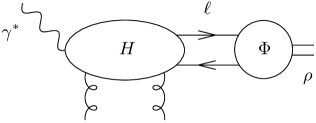
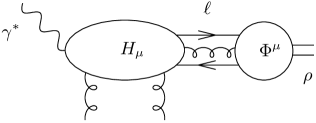
$+\cdots$

Figure 2: Two- and three-parton correlators attached to a hard scattering amplitude in the specific case of the $\gamma^{*}\to\rho$ impact factor, where vertical lines are hard $t-$ channel gluons in the color singlet state.

Each of these scattering amplitudes is the sum of the convolutions of a hard part (denoted by $H$ and $H_{\mu}$ for two- and three-parton contributions, respectively) that corresponds to the transition of the virtual photon into the constituents of the $\rho$ meson and their interactions with off-shell gluons of the $t$ channel, and a soft part (denoted by $\Phi$ and $\Phi^{\mu}$) describing the hadronization of the constituent partons into the $\rho$ meson and parameterized up to a given twist by DAs.

3 Helicity amplitudes and polarized cross-sections

3.1 Impact factors $\gamma^{*}_{L,T}\rightarrow\rho_{L,T}$

In the Sudakov basis, the longitudinal and transverse polarizations of the photon are

$$e_{\gamma L}^{\mu}=\frac{1}{Q}(p_{1}^{\mu}+\frac{Q^{2}}{s}p_{2}^{\mu})\,,\qquad\epsilon^{\pm}=\frac{1}{\sqrt{2}}\left(0,\mp 1,-i,0\right)\,.$$ (6)

For $t=t_{\rm min}$ the same parametrization will be used for the $\rho$-meson polarization with obvious substitutions $Q^{2}\to-m_{\rho}^{2}$ and $Q\to m_{\rho}$.

Let us introduce $p$ and $n$, two light-cone vectors such that $p_{\rho}\approx p$ at twist 3 and $p\cdot n=1$. The polarization of the out-going $\rho$ meson is denoted by $e^{*}$. For further use, we denote $R^{*}_{\perp\alpha}=\varepsilon_{\alpha\lambda\beta\delta}\,e_{\perp}^{*\lambda}p^{\beta}\,n^{\delta}$. We use the following convention for the transverse euclidean polarization vectors $\underline{e}^{\pm}$ as in eq. (6)

$$\underline{e}^{\pm}=\frac{1}{\sqrt{2}}\left(\mp 1,-i\right)\,.$$ (7)

The DAs needed to parameterize the $\rho$ meson productions involved in the results of [40] for the impact factors with ${\underline{\Delta}}=0$, according to [40] are: the twist 2 DA $\varphi_{1}(y;\mu_{F}^{2})$ associated to the production of the longitudinal $\rho$ meson, the two-parton twist 3 DAs $\varphi_{1}^{T}(y;\mu_{F}^{2})$, $\varphi_{A}^{T}(y;\mu_{F}^{2})$ and the three-parton twist 3 DAs $B(y_{1},y_{2};\mu_{F}^{2})$ and $D(y_{1},y_{2};\mu_{F}^{2})$ that parameterize the production of a transversely polarized $\rho$ meson. Following [42, 44], we also use the combinations,

$$M(y_{1},y_{2};\mu_{F}^{2}) = \zeta^{V}_{3}(\mu_{F}^{2})\,B(y_{1},y_{2};\mu_{F}^{2})-\zeta^{A}_{3}(\mu_{F}^{2})\,D(y_{1},y_{2};\mu_{F}^{2})\,,$$

$$S(y_{1},y_{2};\mu_{F}^{2}) = \zeta^{V}_{3}(\mu_{F}^{2})\,B(y_{1},y_{2};\mu_{F}^{2})+\zeta^{A}_{3}(\mu_{F}^{2})\,D(y_{1},y_{2};\mu_{F}^{2})\,,$$ (8)

where $\zeta^{V}_{3}(\mu_{F}^{2})$ and $\zeta^{A}_{3}(\mu_{F}^{2})$ are the dimensionless coupling constants

$$\zeta^{V}_{3}(\mu_{F}^{2})=\frac{f^{V}_{3\rho}(\mu_{F}^{2})}{f_{\rho}}\,,\qquad\zeta^{A}_{3}(\mu_{F}^{2})=\frac{f^{A}_{3\rho}(\mu_{F}^{2})}{f_{\rho}}\,.$$ (9)

The scale $\mu_{F}$ is the factorization scale involved in the production of the $\rho$ meson, that we put equal to the renormalization scale of the evolution of the DAs. We recall in appendix A.1 some basics features of the chiral even twist 2 and twist 3 DAs present in this approach; more details can be found on the DAs in ref. [40]. We recall also in appendix A.2 the dependence of the DAs on the collinear factorization scale $\mu_{F}$ which is driven by the renormalization evolution equations given in ref. [50].

We have recently shown in [44] that these impact factors, expressed in the impact parameter space, read,

$$\Phi^{\gamma^{*}_{L}\to\rho_{L}} = -\frac{1}{4}m_{\rho}f_{\rho}\int dy\int d^{2}{\underline{r}}\left(e^{*}\cdot n\right)\varphi_{1}(y;\mu_{F}^{2})\tilde{H}_{q{\bar{q}}}^{/\!\!\!p_{1}}(y,{\underline{r}},{\underline{k}})\,,$$ (10)

and

$$\Phi^{\gamma^{*}_{T}\to\rho_{T}} = -\frac{1}{4}m_{\rho}f_{\rho}\int dy_{2}\int d^{2}{\underline{r}}\left\{\varphi_{3}(y_{2};\mu_{F}^{2})\tilde{H}_{q{\bar{q}}}^{/\!\!\!e^{*}_{\perp}}(y_{2},{\underline{r}},{\underline{k}})+i\varphi^{T}_{1}(y_{2};\mu_{F}^{2})\left({\underline{e}}^{*}\cdot{\underline{r}}\right)\tilde{H}_{q{\bar{q}}}^{/\!\!\!p_{1}}(y_{2},{\underline{r}},{\underline{k}})\right.$$ (11)

$$\hskip 42.67912pt+\left.i\varphi_{A}(y_{2};\mu_{F}^{2})\tilde{H}_{q{\bar{q}}}^{\,/\!\!\!\!R^{*}_{\perp}\gamma_{5}}(y_{2},{\underline{r}},{\underline{k}})-\varphi^{T}_{A}(y_{2};\mu_{F}^{2})\left(\underline{R}^{*}\cdot{\underline{r}}\right)\tilde{H}_{q{\bar{q}}}^{/\!\!\!p_{1}\gamma_{5}}(y_{2},{\underline{r}},{\underline{k}})\right.$$

$$\hskip 42.67912pt-\left.i\int_{0}^{y_{2}}dy_{1}\int d^{2}\underline{r}^{\prime}\,\left(\zeta^{V}_{3}B(y_{1},y_{2};\mu_{F}^{2})\tilde{H}^{e^{*}_{\perp},/\!\!\!p_{1}}_{q{\bar{q}}g}(y_{1},y_{2},{\underline{r}},\underline{r}^{\prime},{\underline{k}})\right.\right.$$

$$\hskip 128.0374pt\left.\left.+i\zeta^{A}_{3}D(y_{1},y_{2};\mu_{F}^{2})\tilde{H}^{R^{*}_{\perp},/\!\!\!p_{1}\gamma_{5}}_{q{\bar{q}}g}(y_{1},y_{2},{\underline{r}},\underline{r}^{\prime},{\underline{k}})\right)\right\}\,,$$

where we have respectively denoted in the case of two-parton exchange as $y$ and $\bar{y}=1-y$ the longitudinal momentum fractions of the quark and the antiquark, and in the three-parton exchange $y_{1}$, ${\bar{y}}_{2}=1-y_{2}$ and $y_{g}=y_{2}-y_{1}$ the longitudinal momentum fractions of the quark, the antiquark and the gluon. The transverse displacement vectors of the color dipole configurations are denoted as ${\underline{r}}$ for the interacting dipole (two- and three-parton Fock component) and ${\underline{r}}^{\prime}$ for the spectator dipole (present only in the three-parton Fock component). Note that $\left|{\underline{r}}\right|$ in the case of the two-parton component is the transverse size of the quark anti-quark colorless pair. The functions denoted

$$\tilde{H}_{q{\bar{q}}}^{\Gamma^{\mu}b_{\mu}}\equiv\tilde{H}_{q{\bar{q}}}^{\Gamma^{\mu}}b_{\mu}\,,\quad\tilde{H}^{c,\Gamma^{\mu}b_{\mu}}_{q{\bar{q}}g}\equiv\tilde{H}_{q{\bar{q}}g}^{\alpha,\Gamma^{\mu}}\,c_{\alpha}\,b_{\mu}\,,$$ (12)

are the Fourier transforms in the transverse plane of the two-parton component hard parts $H$ and the three-parton component hard parts $H_{\mu}$ (illustrated in figure 2), projected on the appropriate Fierz structures $\Gamma^{\mu}$.

The computations of the hard parts lead to the following generic expressions,

$$\Phi^{\gamma^{*}_{L}\rightarrow\rho_{L}}({\underline{k}},Q,\mu_{F}^{2}) = \left(\frac{\delta^{ab}}{2}\right)\int dy\int d{\underline{r}}\,\,\psi^{\gamma^{*}_{L}\to\rho_{L}}_{(q{\bar{q}})}(y,{\underline{r}};Q,\mu_{F}^{2})\,\mathcal{A}({\underline{r}},{\underline{k}})\,,$$ (13)

$$\Phi^{\gamma^{*}_{T}\rightarrow\rho_{T}}({\underline{k}},Q,\mu_{F}^{2}) = \left(\frac{\delta^{ab}}{2}\right)\int dy\int d{\underline{r}}\,\,\psi^{\gamma^{*}_{T}\to\rho_{T}}_{(q{\bar{q}})}(y,{\underline{r}};Q,\mu_{F}^{2})\,\mathcal{A}({\underline{r}},{\underline{k}})$$

$$+\left(\frac{\delta^{ab}}{2}\right)\int dy_{2}\int dy_{1}\int d{\underline{r}}\,\,\psi^{\gamma^{*}_{T}\to\rho_{T}}_{(q{\bar{q}}g)}(y_{1},y_{2},{\underline{r}};Q,\mu_{F}^{2})\mathcal{A}({\underline{r}},{\underline{k}})\,,$$

where the function

$$\mathcal{A}({\underline{r}},{\underline{k}})=\frac{4\pi\alpha_{s}}{N_{c}}\left(1-\exp\left(i{\underline{k}}\cdot{\underline{r}}\right)\right)\left(1-\exp\left(-i{\underline{k}}\cdot{\underline{r}}\right)\right)\,,$$ (15)

is the scattering amplitude of a quark-antiquark color dipole with the two $t-$channel gluons, putting apart the color factor $Tr(t^{a}\,t^{b})=\delta^{ab}/2$, with $a$ and $b$ color indices and $N_{c}$ the number of colors. The functions $\psi^{\gamma^{*}_{L}\to\rho_{L}}_{(q{\bar{q}})}$, $\psi^{\gamma^{*}_{T}\to\rho_{T}}_{(q{\bar{q}})}$, $\psi^{\gamma^{*}_{T}\to\rho_{T}}_{(q{\bar{q}}g)}$ are respectively the amplitudes of production of a $\rho$ meson from a quark-antiquark (quark-antiquark gluon) system produced far upstream the target in the fluctuation of the virtual photon. These functions are computed up to twist 3 in the collinear aproximation in ref. [44] and they contain information about the relevant color dipole system that interacts with the target. The functions $\psi^{\gamma^{*}_{L,T}\to\rho_{L,T}}_{(q{\bar{q}})}$ can be expressed in terms of the virtual photon wave functions $\Psi_{(h,\bar{h})}^{\gamma^{*}_{L,T}}$,

$$\Psi_{(h,\bar{h})}^{\gamma^{*}_{L}}(y,{\underline{r}};Q^{2}) = \delta_{\bar{h},-h}\frac{e}{2\pi}\sqrt{\frac{N_{c}}{\pi}}\frac{\mu^{2}}{Q}K_{0}(\mu\left|{\underline{r}}\right|)\,,$$ (16)

$$\Psi_{(h,\bar{h})}^{\gamma^{*}_{T}\,(\lambda_{\gamma})}(y,{\underline{r}};Q^{2}) = \delta_{\bar{h},-h}\frac{ie}{2\pi}\sqrt{\frac{N_{c}}{\pi}}(y\delta_{h,\lambda_{\gamma}}+{\bar{y}}\delta_{h,-\lambda_{\gamma}})\frac{({\underline{r}}\cdot{\underline{e}}^{(\lambda_{\gamma})})}{\left|{\underline{r}}\right|}\mu K_{1}(\mu\left|{\underline{r}}\right|)\,,$$ (17)

where $h=\pm\frac{1}{2}$, $\bar{h}=\pm\frac{1}{2}$ denote respectively the helicities of the exchanged quark and anti-quark, and of the combinations of DAs of the $\rho$ meson $\phi^{\rho_{L,T}}_{(h\bar{h})}$,

$$\phi^{\rho_{L}}_{(h,\bar{h})}(y;\mu_{F}^{2}) = \delta_{\bar{h},-h}\sqrt{\frac{\pi}{4N_{c}}}(e_{L}^{*}\cdot n)\varphi_{1}(y;\mu_{F}^{2})\,,$$ (18)

$$\phi_{(h,\bar{h})}^{\rho_{T},\,(\lambda_{\rho})}(y,{\underline{r}};\mu_{F}^{2}) = -\delta_{\bar{h},-h}i\sqrt{\frac{\pi}{4N_{c}}}({\underline{e}}^{(\lambda_{\rho})*}\cdot{\underline{r}})$$ (19)

$$\times \left(\varphi_{A}^{T}(y;\mu_{F}^{2})+(\delta_{h,\lambda_{\rho}}-\delta_{h,-\lambda_{\rho}})\varphi_{1}^{T}(y;\mu_{F}^{2})\right)\,.$$

In the two-parton approximation, these functions $\phi^{\rho_{L}}_{(h,\bar{h})}(y;\mu_{F}^{2})$ and $\phi_{(h,\bar{h})}^{\rho_{T},\,(\lambda_{\rho})}(y,{\underline{r}};\mu_{F}^{2})$ parameterize the moments of the wave functions of the $\rho$ meson, i.e. the first terms of the Taylor expansion of the wave functions at small ${\underline{r}}$. Note that in the approach of ref. [38] $\phi^{\rho_{L}}_{(h,\bar{h})}(y;\mu_{F}^{2})$ and $\phi_{(h,\bar{h})}^{\rho_{T},\,(\lambda_{\rho})}(y,{\underline{r}};\mu_{F}^{2})$ are replaced by the Taylor expansion for small ${\underline{r}}$ of the modeled wave functions of the vector mesons. Finally, the functions $\psi^{\gamma^{*}_{L}\to\rho_{L}}_{(q{\bar{q}})}$ and $\psi^{\gamma^{*}_{T}\to\rho_{T}}_{(q{\bar{q}})}$ with two-parton components read

$$\psi^{\gamma^{*}_{L}\to\rho_{L}}_{(q{\bar{q}})}(y,{\underline{r}};Q,\mu_{F}^{2}) = \frac{m_{\rho}f_{\rho}}{\sqrt{2}}\sum_{(h,\bar{h})}\phi^{\rho_{L}}_{(h\bar{h})}(y;\mu_{F}^{2})\,\Psi_{(h,\bar{h})}^{\gamma^{*}_{L}}(y,{\underline{r}};Q^{2})\,,$$ (20)

$$\psi^{\gamma^{*}_{T}\to\rho_{T}}_{(q{\bar{q}})}(y,{\underline{r}};Q,\mu_{F}^{2}) = \frac{m_{\rho}f_{\rho}}{\sqrt{2}}\sum_{(h,\bar{h})}\phi^{\rho_{T},\,(\lambda_{\rho})}_{(h,\bar{h})}(y;\mu_{F}^{2})\,\Psi_{(h,\bar{h})}^{\gamma^{*}_{T}\,(\lambda{\gamma})}(y,{\underline{r}};Q^{2})\,.$$ (21)

The function $\psi^{\gamma^{*}_{T}\to\rho_{T}}_{(q{\bar{q}}g)}$ with three-parton components reads

$$\psi^{\gamma^{*}_{T}\to\rho_{T}}_{(q{\bar{q}}g)}(y,{\underline{r}};Q,\mu_{F}^{2}) = \frac{m_{\rho}f_{\rho}}{\sqrt{2}}\left[\left(\sqrt{\frac{\pi}{4N_{c}}}\frac{S(y_{1},y_{2};\mu_{F}^{2})}{2}\right)\mathcal{F}^{\gamma^{*}_{T}}(y_{1},y_{2},{\underline{r}};Q)\right.$$ (22)

$$\hskip 42.67912pt-\left.\left(\sqrt{\frac{\pi}{4N_{c}}}\frac{M(y_{1},y_{2};\mu_{F}^{2})}{2}\right)\mathcal{F}^{\gamma^{*}_{T}}({\bar{y}}_{2},{\bar{y}}_{1},{\underline{r}};Q)\right]\,,$$

where the function $\mathcal{F}^{\gamma^{*}_{T}}$ describes the fluctuation of the transversely polarized photon into a quark-antiquark-gluon color singlet. The function $\mathcal{F}^{\gamma^{*}_{T}}$ can be expressed in terms of the longitudinally polarized photon wave function

$$\Psi^{\gamma^{*}_{L}}(\mu_{i},{\underline{r}};Q)=\sum_{(h,\bar{h})}\Psi_{(h,\bar{h})}^{\gamma^{*}_{L}}\equiv 2\frac{e}{2\pi}\sqrt{\frac{N_{c}}{\pi}}\frac{\mu_{i}^{2}}{Q}K_{0}(\mu_{i}\left|{\underline{r}}\right|)\,,$$ (23)

as

$$\mathcal{F}^{\gamma^{*}_{T}}(y_{1},y_{2},{\underline{r}};Q)=\frac{1}{2}\left\{2\,\left[\frac{\Psi^{\gamma^{*}_{L}}(\mu_{1},{\underline{r}};Q)}{{\bar{y}}_{1}Q}\right]\right.$$

$$\left.+\frac{N_{C}}{C_{F}}\left[\,\frac{\Psi^{\gamma^{*}_{L}}(\mu_{{\bar{q}}g},{\underline{r}};Q)}{{\bar{y}}_{1}Q}+\left(\frac{y_{2}\,{\bar{y}}_{1}}{{\bar{y}}_{2}\,y_{1}}\right)\times\left(\frac{\Psi^{\gamma^{*}_{L}}(\mu_{2},{\underline{r}};Q)}{{\bar{y}}_{1}Q}-\frac{\Psi^{\gamma^{*}_{L}}(\mu_{{\bar{q}}g},{\underline{r}};Q)}{{\bar{y}}_{1}Q}\right)\right]\right.$$

$$+\left.\left(\frac{N_{C}}{C_{F}}-2\right)\left[\left(\frac{\Psi^{\gamma^{*}_{L}}(\mu_{1},{\underline{r}};Q)}{y_{g}Q}-\frac{\Psi^{\gamma^{*}_{L}}(\mu_{q{\bar{q}}},{\underline{r}};Q)}{y_{g}Q}\right)\right.\right.$$

$$\left.\left.\hskip 71.13188pt+\frac{y_{2}}{{\bar{y}}_{2}}\left(\frac{\Psi^{\gamma^{*}_{L}}(\mu_{2},{\underline{r}};Q)}{y_{g}Q}-\frac{\Psi^{\gamma^{*}_{L}}(\mu_{q{\bar{q}}},{\underline{r}};Q)}{y_{g}Q}\right)\right]\right\}\,,$$ (24)

with

$$\mu_{1}^{2}=y_{1}{\bar{y}}_{1}Q^{2}\,, \mu_{2}^{2}=y_{2}{\bar{y}}_{2}Q^{2}\,,$$ (25)

$$\mu_{qg}^{2}=\frac{y_{1}y_{g}}{y_{1}+y_{g}}Q^{2}\,,\quad\mu_{{\bar{q}}g}^{2} = \frac{{\bar{y}}_{2}y_{g}}{{\bar{y}}_{2}+y_{g}}Q^{2}\,,\quad\mu_{q{\bar{q}}}^{2}=\frac{y_{1}{\bar{y}}_{2}}{y_{1}+{\bar{y}}_{2}}Q^{2}\,,$$

and $C_{F}=\frac{N_{c}^{2}-1}{2N_{c}}$. Note, that in the large $N_{C}$ limit $\mathcal{F}^{\gamma^{*}_{T}}$ simplifies,

$$\mathcal{F}^{\gamma^{*}_{T}}(y_{1},y_{2},{\underline{r}};Q)\xrightarrow[N_{C}\to\infty]{}\frac{1}{{\bar{y}}_{1}y_{1}{\bar{y}}_{2}Q}$$ (26)

$$\times\left\{y_{1}{\bar{y}}_{2}\Psi^{\gamma^{*}_{L}}(\mu_{1},{\underline{r}};Q)+y_{2}{\bar{y}}_{1}\Psi^{\gamma^{*}_{L}}(\mu_{2},{\underline{r}};Q)-y_{g}\Psi^{\gamma^{*}_{L}}(\mu_{{\bar{q}}g},{\underline{r}};Q)\right\}\,.$$

3.2 From impact factors to helicity amplitudes and polarized cross-sections

According to eq. (5), the helicity amplitudes read,

$$\frac{T_{\lambda_{\rho},\lambda_{\gamma}}}{s}=\frac{\delta^{ab}}{2}\int\frac{d^{2}{\underline{k}}}{{\underline{k}}^{4}}\Phi_{ab}^{\gamma^{*}_{\lambda_{\gamma}}\rightarrow\rho_{\lambda_{\rho}}}({\underline{k}},Q,\mu_{F}^{2})\mathcal{F}(x,{\underline{k}})\,.$$ (27)

Inserting the expressions for the impact factor $\Phi^{\gamma^{*}_{\lambda_{\gamma}}\rightarrow\rho_{\lambda_{\rho}}}$ of eqs. (13, 3.1), one gets

$$\frac{T_{00}}{s} = \int dy\int d{\underline{r}}\,\psi^{\gamma^{*}_{L}\to\rho_{L}}_{(q{\bar{q}})}(y,{\underline{r}};Q,\mu_{F}^{2})\,\hat{\sigma}(x,{\underline{r}})\,,$$ (28)

$$\frac{T_{11}}{s} = \int dy\int d{\underline{r}}\,\psi^{\gamma^{*}_{T}\to\rho_{T}}_{(q{\bar{q}})}(y,{\underline{r}};Q,\mu_{F}^{2})\,\hat{\sigma}(x,{\underline{r}})$$

$$+\int dy_{2}\int dy_{1}\int d{\underline{r}}\,\psi^{\gamma^{*}_{T}\to\rho_{T}}_{(q{\bar{q}}g)}(y_{1},y_{2},{\underline{r}};Q,\mu_{F}^{2})\,\hat{\sigma}(x,{\underline{r}})\,,$$

where we have identified the dipole cross-section as defined in ref. [56]

$$\hat{\sigma}(x,{\underline{r}}) = \frac{N_{c}^{2}-1}{4}\int\frac{d^{2}{\underline{k}}}{{\underline{k}}^{4}}\mathcal{F}(x,{\underline{k}})\mathcal{A}({\underline{k}},{\underline{r}})\,.$$ (30)

Note that we can separate the $T_{11}$ as the WW contribution and the genuine contribution,

$$\frac{T^{WW}_{11}}{s} = \int dy\int d{\underline{r}}\,\psi^{\gamma^{*}_{T}\to\rho_{T},\,WW}_{(q{\bar{q}})}(y,{\underline{r}};Q,\mu_{F}^{2})\,\hat{\sigma}(x,{\underline{r}})\,,$$ (31)

$$\frac{T^{gen}_{11}}{s} = \int dy\int d{\underline{r}}\,\psi^{\gamma^{*}_{T}\to\rho_{T},\,gen}_{(q{\bar{q}})}(y,{\underline{r}};Q,\mu_{F}^{2})\,\hat{\sigma}(x,{\underline{r}})$$

$$+\int dy_{2}\int dy_{1}\int d{\underline{r}}\,\psi^{\gamma^{*}_{T}\to\rho_{T}}_{(q{\bar{q}}g)}(y_{1},y_{2},{\underline{r}};Q,\mu_{F}^{2})\,\hat{\sigma}(x,{\underline{r}})\,,$$

The formulas (28, 3.2) allow us to combine various models of the scattering amplitude of a dipole on a nucleon with the results obtained by twist expansion of the $\gamma^{*}\to\rho$ impact factor. At $t=t_{\rm min}$ the contribution to the cross-sections $\sigma_{L}$ and $\sigma_{T}$ are respectively coming from the helicity amplitudes $T_{00}$ and $T_{11}$,

$$\frac{d\sigma_{L}}{dt}(t=0) = \frac{\left|T_{00}(s,t=0)\right|^{2}}{16\pi s^{2}}\,,$$ (33)

$$\frac{d\sigma_{T}}{dt}(t=0) = \frac{\left|T_{11}(s,t=0)\right|^{2}}{16\pi s^{2}}\,.$$ (34)

The $t-$dependency is expected to be governed by non-perturbative effects of the nucleon, which can be phenomenologically parameterized by an exponential dependence of the differential cross-section

$$\frac{d\sigma_{L,T}}{dt}(t)=e^{-b(Q^{2})t}\,\frac{d\sigma_{L,T}}{dt}(t=0)\,.$$ (35)

This results in the polarized cross-sections

$$\sigma_{L} = \frac{1}{b(Q^{2})}\frac{\left|T_{00}(s,t=0)\right|^{2}}{16\pi s^{2}}\,,$$ (36)

$$\sigma_{T} = \frac{1}{b(Q^{2})}\frac{\left|T_{11}(s,t=0)\right|^{2}}{16\pi s^{2}}\,.$$ (37)

The $b(Q^{2})$ slope has been measured by ZEUS and H1. We will use here quadratic fits of the $b(Q^{2})$ slope data of ref. [4] to determine the cross-section.

In the following section, we will briefly present the dipole models we shall use to compare our predictions with HERA data. Note that we could in principle use a dipole model taking into account skewness effects. This skewness dependence can be implemented along approaches of refs. [60, 61], but this subleading physical effects will be neglected in the present study.

4 Dipole models

In the dipole picture, the DIS cross-section reads [23, 24]

$$\sigma^{\gamma^{*}p}_{L,T} = \int d^{2}{\underline{r}}\int dy\sum^{N_{f}}_{\text{f}}\left|\Psi^{\gamma^{*}_{L,T}}_{f}(y,{\underline{r}};Q)\right|^{2}\,\hat{\sigma}(x,{\underline{r}})\,,$$ (38)

with

$$\hat{\sigma}(x,{\underline{r}}) = \int d^{2}\underline{b}\,\frac{d\hat{\sigma}_{q{\bar{q}}}}{d^{2}\underline{b}}=2\int d^{2}\underline{b}\,\,\mathcal{N}(x,{\underline{r}},\underline{b})\,.$$ (39)

The low-$x$ saturation dynamics of the nucleon target was first introduced in refs. [52, 62] by Golec-Biernat and Wüsthoff (GBW) model to describe the inclusive and diffractive structure functions of DIS, which inspired many phenomenological descriptions of DIS HERA data [63, 64, 65, 55, 66, 47, 67]. In this model the dipole cross-section reads

$$\hat{\sigma}(x,r)=\sigma_{0}\left\{1-\exp\left(-\frac{r^{2}}{4R_{0}^{2}(x)}\right)\right\}\,,$$ (40)

where

$$R_{0}^{2}(x)=\frac{1}{\text{GeV}^{2}}\left(\frac{x}{x_{0}}\right)^{\lambda_{p}}\,,$$ (41)

and it involves three independent parameters $\left\{\sigma_{0},x_{0},\lambda_{p}\right\}$. One can see from eq. (38) that since the wave functions are peaked at $r\sim\frac{1}{Q}$, the domain in which the saturation effects are significant is given by

$$Q^{2}\lesssim\frac{1}{R_{0}^{2}(x)}\equiv Q_{S}^{2}(x)\,.$$ (42)

To make contact with photoproduction, it is customary [52] to make the following modification of the definition of the Bjorken variable $x$

$$x\to x\left(1+\frac{4\,m_{f}^{2}}{Q^{2}}\right)=\frac{Q^{2}}{W^{2}+Q^{2}}\left(1+\frac{4\,m_{f}^{2}}{Q^{2}}\right)\xrightarrow[Q^{2}\to 0]{}\frac{4\,m_{f}^{2}}{W^{2}}\,,$$ (43)

where $m_{f}$ is an effective quark mass which depends on the flavour $f$ and of the model used to fit the data. This modification is adopted in the following.

In the GBW saturation model, light quark masses are taken to be $0.14\;$GeV in order to get a good fit of the photoproduction region. The inclusion of the charm contribution, with $m_{c}=1.5\;$GeV has also been performed in ref. [52]. The normalisation $\sigma_{0}$ results from the integration over the impact parameter $b$, assuming that the $b-$dependence of the dipole amplitude factorises as $\mathcal{N}(x,{\underline{r}},\underline{b})=T(\underline{b})\,\mathcal{N}(x,r)$, where $T(b)$ is related to the density of gluon within the target, leading to

$$\hat{\sigma}(x,{\underline{r}}) = 2\int d^{2}\underline{b}\,T(\underline{b})\,\mathcal{N}(x,r)=\sigma_{0}\,\mathcal{N}(x,r)\,.$$ (44)

This model provides a good description of inclusive and diffractive structure functions for the values of the parameters presented in table 1.

Fits	$\sigma_{0}$ (mb)	$\lambda_{p}$	$x_{0}$
No charm	23.03	0.288	$3.04\times 10^{-4}$
With charm	29.12	0.277	$0.41\times 10^{-4}$

Table 1: Values of the parameters entering the GBW dipole cross-section.

The small $x$ evolution of the dipole cross-section can be modeled as in the refs. [52], or computed numerically from the running coupling Balitsky-Kovchegov (rcBK) equation. Indeed, the $x-$dependence is driven at small $x$ by perturbative non-linear equations, the Jalilian-Marian-Iancu-McLerran-Weigert-Leonidov-Kovner (JIMWLK) equation [68, 69, 70, 71, 72, 73] and the Balitsky-Kovchegov (BK) equation [74, 75]. The solutions of the two equations are not significantly different and the BK equation is simpler to solve numerically than the JIMWLK equation. The LO-BK equation cannot be used to obtain the low $x$ evolution as it predicts a growth of the saturation scale much faster than the growth expected from the anlysis based on phenomenological models. It was shown in [53, 54] that taking into account only the running coupling corrections of the evolution kernel allows to get the main higher order contributions, and to solve the discrepancy between the growths of the saturation scale. A numerical solution of the running coupling BK (rcBK) equation was obtained in refs. [76, 77] based on initial conditions inspired by the GBW model [52] and the McLerran-Venugopalan (MV) model [78]. We will denote these numerical solutions for the dipole scattering amplitudes as the Albacete-Armesto-Milhano-Quiroga-Salgado (AAMQS)-model.

$$\mathcal{N}^{GBW}(x_{0},r) = \sigma_{0}^{GBW}\left\{1-\exp\left[-\left(\frac{r^{2}Q^{2}_{s\,0}}{4}\right)^{\gamma}\right]\right\}\,,$$ (45)

$$\mathcal{N}^{MV}(x_{0},r) = \sigma_{0}^{MV}\left\{1-\exp\left[-\left(\frac{r^{2}Q^{2}_{s\,0}}{4}\right)^{\gamma}\,\ln\left(\frac{r}{\Lambda_{QCD}}+e\right)\right]\right\}\,,$$ (46)

with $x_{0}=0.01$ and $Q_{s\,0}$ the initial saturation scale at $x=x_{0}$, and $\gamma$ the anomalous dimension. The coupling constant in the evolution kernel of the rcBK equation depends on the number of active quark flavors $n_{f}$,

$$\alpha_{s,n_{f}}(r^{2}) = \frac{4\pi}{\beta_{0,n_{f}}\,\ln\left[\frac{4C^{2}}{r^{2}\Lambda^{2}_{n_{f}}}\right]}\,,$$ (47)

where $\beta_{0,n_{f}}=11-\frac{2}{3}n_{f}$, $\Lambda_{n_{f}}$ is the QCD scale and $C$ is one of the free parameters of the model. As usual, the scales $\Lambda_{n_{f}}$ are determined by the matching condition $\alpha_{s,n_{f}-1}(r_{\star}^{2})=\alpha_{s,n_{f}}(r_{\star}^{2})$ at $r_{\star}^{2}=4C^{2}/m_{f}^{2}$ and an experimental value of $\alpha_{s}$. In eq. (46), the scale $\Lambda_{QCD}$ is identified with $\Lambda_{3}$.

The parameters are fitted to the experimental data for the inclusive structure function of DIS

$$F_{2}(x,Q^{2})=\frac{Q^{2}}{4\pi^{2}\alpha_{em}}\left(\sigma_{T}+\sigma_{L}\right)\,,$$ (48)

and give a good description for the data of the longitudinal structure function

$$F_{L}(x,Q^{2})=\frac{Q^{2}}{4\pi^{2}\alpha_{em}}\sigma_{L}\,.$$ (49)

Two sets of dipole cross-sections are available for each of the initial conditions. The first set of dipole cross-sections respectively denoted as (a) and (e) for the GBW and the MV initial conditions, are fitted to data by taking only into account the light quarks $u,d,s\,.$ The second set, respectively denoted as (b) and (f) for the GBW and the MV initial conditions, are fitted taking into account the dipole cross-section of the light quarks $\sigma_{0}\,\mathcal{N}^{\text{l.}}(x,{\underline{r}})$ and of the heavy quarks $\sigma_{0}^{\rm h}\mathcal{N}^{\text{h.}}(x,{\underline{r}})\,.$ The normalization of the dipole cross-section $\sigma_{0}^{{\rm h.}}$ for the charm and the bottom quarks are assumed to be equal. Thus the cross-sections read

$$\sigma^{\gamma^{*}p}_{L,T;\,\text{set(a),(e)}} = \sigma_{0}\sum_{\text{f=u,d,s}}\int d^{2}{\underline{r}}\int dy\left|\Psi^{\gamma^{*}_{L,T}}_{f}(y,{\underline{r}};Q,m_{f},e_{f})\right|^{2}\,\mathcal{N}^{\text{l.}}(x,{\underline{r}})\,,$$ (50)

$$\sigma^{\gamma^{*}p}_{L,T,\,\text{set(b),(f)}} = \sigma_{0}^{l.}\sum_{\text{f=u,d,s}}\int d^{2}{\underline{r}}\int dy\left|\Psi^{\gamma^{*}_{L,T}}_{f}(y,{\underline{r}};Q,m_{f},e_{f})\right|^{2}\,\mathcal{N}^{\text{l.}}(x,{\underline{r}})$$ (51)

$$+ \sigma_{0}^{h.}\sum_{\text{f=c,b}}\int d^{2}{\underline{r}}\int dy\left|\Psi^{\gamma^{*}_{L,T}}_{f}(y,{\underline{r}};Q,m_{f},e_{f})\right|^{2}\,\mathcal{N}^{\text{h.}}(x,{\underline{r}})\,.$$

In the following parts we will focus mostly on the sets (a) and (b) using the GBW initial condition respectively denoted as AAMQSa and AAMQSb, as the effects due to different initial conditions do not involve significant changes in the numerical results of present study. We present in Tabs. 2 and 3 values of the parameters of the fits obtained in ref. [77].

Fits	$Q_{s0}^{2}$	$\sigma_{0}$ (mb)	$\gamma$	$C$	$\chi^{2}/N_{df}$
(a)	0.241	32.357	0.971	2.46	1.226
(e)	0.165	32.895	1.135	2.52	1.171

Table 2: Values of the parameters entering the AAMQS sets (a) and (e) dipole cross-sections.

Fits	$Q_{s0}^{2}$	$Q_{s0}^{(c,b)\,2}$	$\sigma_{0}^{{\rm l.}}$ (mb)	$\sigma_{0}^{{\rm h.}}$ (mb)	$\gamma$	$\gamma^{(c,b)}$	$C$	$\chi^{2}/N_{df}$
(b)	0.2386	0.2329	35.465	18.430	1.263	0.883	3.902	1.231
(f)	0.1687	0.1417	35.449	19.066	1.369	1.035	4.079	1.244

Table 3: Values of the parameters entering the AAMQS sets (b) and (f) dipole cross-sections.

Note that the models of dipole cross-section we use here involve only a quark anti-quark intermediate state between the initial and final wave functions used to describe DIS process while the impact factor $\gamma^{*}_{T}\to\rho_{T}$ involves also $q{\bar{q}}g$ partonic state. The error induced by this approximation should be subleading compare to higher twist corrections or the choice of $\mu_{F}$, but still it is difficult to appreciate quantitatively how much it could impact on the predictions.

For completeness, we will also display predictions using the Gunion and Soper model (GS-model) [43]. This model was used in our first phenomenological study of ref. [42], and it assumes that the hadron impact factor takes the form

$$\Phi^{N\to N}(\underline{k},{\underline{\Delta}};M^{2})=A\,\delta_{ab}\left[\frac{1}{M^{2}+(\frac{{\underline{\Delta}}}{2})^{2}}-\frac{1}{M^{2}+(\underline{k}-\frac{{\underline{\Delta}}}{2})^{2}}\right]\,,$$ (52)

where $A$ and $M$ are free parameters that correspond to the soft scales of the proton-proton impact factor. As it was discussed in [42], the ratios of helicity amplitudes are well described for $M\simeq 1\;$GeV and the result is not very sensitive to this parameter. Note that this impact factor indeed vanishes when $\underline{k}\to 0$ or ${\underline{\Delta}}-\underline{k}\to 0$ in a minimal way. Such a model was the basis of the dipole approach of high energy scattering [79] and used successfully for describing deep inelastic scattering (DIS) at small $x$ [80]. The dipole-proton scattering amplitude in the two-gluon exchange approximation, computed in details in appendix A.3, resulting from the GS-model for the proton impact factor is:

$$\mathcal{N}({\underline{r}},M) = \int\frac{d^{2}{\underline{k}}}{(2\pi)^{2}}\frac{1}{({\underline{k}}^{2})^{2}}\,A\delta_{ab}\left(\frac{1}{M^{2}}-\frac{1}{M^{2}+{\underline{k}}^{2}}\right)\left(1-e^{i{\underline{k}}\cdot{\underline{r}}}\right)\left(1-e^{-i{\underline{k}}\cdot{\underline{r}}}\right)$$ (53)

$$= \frac{A\delta_{ab}}{\pi M^{4}}\left(\gamma+\ln\frac{M\,r}{2}+K_{0}(M\,r)\right)\,.$$ (54)

5 Comparison with the HERA data

Our main results are the polarized cross-sections $\sigma_{T}$ and $\sigma_{L}$ of the process (1), that we compare with the data of the H1 collaboration [4].

(a) $\sigma_{T}$ vs H1 data

(b) $\sigma_{L}$ vs H1 data

Figure 3: Predictions for $\sigma_{T}$ and $\sigma_{L}$ vs $Q^{2}$, for $W=75\;$GeV, using the AAMQSa (red solid line), AAMQSb (blue large dashed line) and GBW (green dashed line) models compared to the data of H1[4].

In the following plots, experimental errors are taken to be the quadratic sum of statistical and systematical errors. The collinear factorization scale $\mu_{F}$ only appears in the scattering amplitudes through the DAs and the coupling constants and unless specified we will assume that $\mu_{F}$ depends on the virtuality $Q^{2}$ as

$$\mu_{F}^{2}(Q^{2})=\frac{Q^{2}+M_{\rho}^{2}}{4}\xrightarrow[]{Q^{2}>>M_{\rho}^{2}}\frac{Q^{2}}{4}\,.$$ (55)

The figures 3(a) and 3(b) show the full twist 3 predictions respectively for $\sigma_{T}$ and $\sigma_{L}$, using the different dipole models. The results of the predictions for $\sigma_{T}$ (figure 3(a)) and $\sigma_{L}$ (figure 3(b)) are in agreement with the data for values of $Q^{2}$ larger than approximately 7 GeV² for $\sigma_{T}$ and $7$ GeV² for $\sigma_{L}$ depending on the considered dipole model. The results based on the AAMQSa model are giving a slightly better description than with the AAMQSb although both sets give good quality fits of DIS data. The results obtained by GBW model are close to the one obtained by the AAMQSa model; both are in good agreement with the data for $Q^{2}$ above 7 GeV². Let us insist on the fact that the agreement for $Q^{2}\geq 7\;$GeV² of our predictions with data is non-trivial since all free parameters of the dipole cross-section (normalization, $R_{0}(x)$, etc…) are completely fixed by the fit of DIS data, while on the $\rho$ side the normalizations are given by decay constants obtained from QCD sum rules.

Keeping in mind that the results are not too sensitive to the precise choice of the dipole model, below we will focus on the predictions of the AAMQSa model. Some results of the GBW, AAMQSb and GS models are presented in appendix A.4.

(a) AS (purple dashed line), WW (blue long dashed line) and Total (red solid line) contributions to $\sigma_{T}$.

(b) AS (purple dashed line) and Total (red solid line) contributions to $\sigma_{L}$.

Figure 4: Predictions for $\sigma_{T}$ and $\sigma_{L}$ vs $Q^{2}$, for $W=75\;$GeV, using the AAMQSa-model, compared to the data of H1[4].

In figure 4, we show separately three different contributions:

• the full twist 3 (Total) contribution, involving both the WW and the genuine solutions of the DAs.

• the WW contribution, only involving the WW solutions of the DAs.

• the asymptotic (AS) contribution (for $\mu_{F}\to\infty$), involving the asymptotic solutions of the DAs. In this limit the genuine contribution vanishes and the WW DAs can be expressed as functions of the asymptotic DA $\varphi_{1}(y)=6y{\bar{y}}$.

The results of the predictions for $\sigma_{T}$ (figure 4(a)) and $\sigma_{L}$ (figure 4(b)) are in agreement with the data for values of $Q^{2}$ respectively larger than $Q^{2\,{\rm min}}_{T}\sim$ 6.5 GeV² and $Q^{2\,{\rm min}}_{L}\sim 5$ GeV² which confirms that the amplitude factorizes into a universal colour dipole scattering amplitude and that the truncated twist expansion of the $\rho$ meson soft part is justified.

The two scales $Q^{2\,\text{min}}_{T}$ and $Q^{2\,\text{min}}_{L}$ are close to each other. We interpret this fact as an indication that the discrepancy between data and our predictions at low $Q^{2}$ are mainly due to the higher twist contributions to the impact factor from the meson structure rather than an effect of the saturation dynamics of the nucleon which should be well described at this scale by the saturation models. Let us mention, again that these saturation models are known to fit very well inclusive DIS as well as diffractive DIS data (for GBW) at these low $Q^{2}$ values.

The saturation scale, given by $Q_{S}=1/R_{0}(x)$ is of order $1\;$GeV in the kinematics of HERA. Since our predictions are only consistent with data in the region $Q^{2}>Q^{2\,\text{min}}_{L,T}>Q^{2}_{S}$, this limitation do not allow us to access the domain $Q^{2}_{S}\gtrsim Q^{2}$ where saturation effects can be essential.

The predictions are dominated by the WW-contribution and are not very sensitive to the choice of the collinear factorization scale. This will be further discussed in section 6.

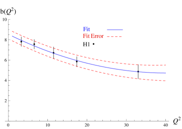
Figure 5: Quadratic fits of the $b-$slope H1 data.

(a) AS (purple) and Total (red) contributions to $\sigma_{T}$.

(b) AS (purple) and Total (red) contributions to $\sigma_{L}$.

Figure 6: Full twist 3 and asymptotic predictions with the $b-$slope uncertainty, using AAMQSa model.

An estimation of the error on the cross-sections caused by the error bars on the $b-$slope measurements is obtained by fitting the upper and lower bounds of the $b-$slope as shown in figure 5, and then by computing the predictions based on these fits as shown in figure 6. Note that we have assumed that the longitudinal $b_{L}$ and the transverse $b_{T}$ slopes are equal to the $b-$slope of the total cross-section. This assumption is supported by H1 data where the measurements of the difference $b_{L}-b_{T}$ for $Q^{2}=3.3\;$GeV² and $Q^{2}=8.6\;$GeV² are much smaller than the $b-$slope value. Let us also emphasize that in this approach we compute the polarized differential cross-sections in the limit $t=t_{\rm min}\approx 0$ where only the $s$-channel helicity conserving (SCHC) amplitudes $T_{00}$ and $T_{11}$ are non-zero. The contributions of other helicity amplitudes are encoded in the phenomenological $t-$dependence given in eq. (35) and it turns out that data for the total differential cross-section are dominated by a $t$-region of very small values, with a typical spread given by the scale $\frac{1}{\left\langle b\right\rangle}\approx\frac{1}{6}\;$GeV².

We now compare our predictions with the data for the total cross-section $\sigma$, given by the sum $\sigma=\sigma_{L}+\sigma_{T}$ according to ZEUS convention in ref. [3] or $\sigma=\varepsilon\sigma_{L}+\sigma_{T}$ following H1 notation [4], where $\varepsilon$ is the photon polarization parameter

$$\varepsilon\simeq(1-y)/(1-y+y^{2}/2)\,.$$ (56)

We show in figures 7(a) and 7(b), the AS, WW and Total contributions to the total cross-section $\sigma$ as function of $Q^{2}$ for fixed averaged $W$. The predictions are larger than the data for $Q^{2}$ smaller than approximately 7 GeV², as expected from the results of $\sigma_{L,T}$.

(a) AS (purple dashed line), WW (blue long dashed line) and Total (red solid line) contributions vs H1 data.

(b) AS (purple dashed line), WW (blue long dashed line) and Total (red solid line) contributions vs ZEUS data.

Figure 7: Predictions for $\sigma$ vs $Q^{2}$ compared respectively with H1[4] data (figure (a)) for $W=75\;$GeV and with ZEUS[3] data (figure (b)) for $W=90\;$GeV, using the AAMQSa-model.

The figures 8(a), 8(b), 9(a) and 9(b) show the $W$ dependence of the cross-section for several values of $Q^{2}$. We see again a good agreement between the predictions and the data for $Q^{2}$ approximately above 6 GeV² for H1 data and 8 GeV² for ZEUS data, taking into account the uncertainty on the $b-$slope.

(a) Asymptotic (purple dashed line), WW (blue long dashed line), total (red solid line) contributions vs H1 data.

(b) Total contribution to $\sigma$ including the $b-$slope errors vs H1 data.

Figure 8: Predictions for $\sigma$ vs $W$, using the AAMQSa-model, compared with H1[4] data. Figure (a): AS, WW and Total contributions. Figure (b): Total contribution taking into account the uncertainties on the $b-$slope.

(a) Asymptotic (purple dashed line), WW (blue long dashed line), total (red solid line) contributions vs ZEUS data.

(b) Total contribution to $\sigma$ including the $b-$slope errors vs ZEUS data.

Figure 9: Predictions for $\sigma$ vs $W$, using the AAMQSa-model, compared with ZEUS[3] data. Figure (a): AS, WW and Total contributions. Figure (b): Total contribution taking into account the uncertainties on the $b-$slope.

Finally, our analysis also provides predictions for the ratios $R$ and for the spin density matrix element $r^{04}_{00}$

$$R = \frac{\sigma_{L}}{\sigma_{T}}\,,$$ (57)

$$r^{04}_{00} = \frac{\sigma_{L}}{\sigma}\,.$$ (58)

Assuming to keep only the SCHC amplitudes $T_{11}$ and $T_{00}$, and the equality of slopes $b_{L}=b_{T}$, the $t-$dependences of the cross-sections cancel in the ratios $R$ and $r^{04}_{00}$, leading to

$$R = \frac{1}{x_{11}^{2}}$$ (59)

and

$$r^{04}_{00} = \frac{\varepsilon}{\varepsilon+x_{11}^{2}}\,,$$ (60)

where $x_{11}=|T_{11}|/|T_{00}|\,.$ H1 and ZEUS measurements of $R$ and $r^{04}_{00}=\sigma_{L}/\sigma$ as functions of $\left|t\right|$ confirm this weak dependence on $\left|t\right|$. Based on H1 data, we can estimate [42] the correction to the ratio $r^{04}_{00}$ due to the amplitude $T_{01},$ for the $t-$range of H1, to be below 1$\%$. The results are shown in figure 10 for the ratio $R$ and in figure 11 for the spin density matrix element $r^{04}_{00}$, using AAMQSa model.

(a) AAMQSa versus H1 data.

(b) AAMQSa versus ZEUS data.

Figure 10: The full twist 3 contribution to the ratio of the cross-sections $R=\sigma_{L}/\sigma_{T}$ in the limit $t=0$ versus $W$ and $Q^{2}$ compared to the data of H1 [4] in figure (a) and ZEUS [3] in figure (b).

(a) Asymptotic (purple dashed line), WW (blue long dashed line), Total (red solid line) contributions using AAMQSa-model vs H1 data.

(b) Asymptotic (purple dashed line), WW (blue long dashed line), Total (red solid line) contributions using AAMQSa-model vs ZEUS data.

Figure 11: Predictions for $r^{04}_{00}$ vs $W$ and $Q^{2}$ compared respectively with H1[4] data (figures (a)) and ZEUS[3] data (figures (b)), using the AAMQSa-model.

6 The radial distributions of dipoles involved in the overlap of the $\gamma^{*}_{L(T)}$ and $\rho_{L(T)}-$meson states

In the dipole picture, the overlap of the wave functions of the outgoing $\rho$ meson $\Psi_{(h,\bar{h})}^{*\rho_{L,T}\,(\lambda_{\rho})}$ and of the incoming virtual photon $\Psi_{(h,\bar{h})}^{\gamma^{*}_{L,T}\,(\lambda_{\gamma})}$ represents the amplitude of probability for these states to dissociate into a quark anti-quark color dipole of size ${\underline{r}}$, the quark having a longitudinal momentum fraction $y$. We define thus the probability amplitude $\mathcal{W}_{\lambda_{\rho}\lambda_{\gamma}}$ as the corresponding parts of the impact factors appearing in eqs. (28) and (3.2),

$$\mathcal{W}_{00}(y,r;\mu_{F}^{2},Q^{2})=\psi^{\gamma^{*}_{L}\to\rho_{L}}_{(q{\bar{q}})}(y,{\underline{r}};Q,\mu_{F}^{2})\,,$$ (61)

for the amplitude $T_{00}$ and

$$\mathcal{W}_{11}(y,r;\mu_{F}^{2},Q^{2}) = \psi^{\gamma^{*}_{T}\to\rho_{T}}_{(q{\bar{q}})}(y,{\underline{r}};Q,\mu_{F}^{2})+\int_{0}^{y}dy_{1}\,\psi^{\gamma^{*}_{T}\to\rho_{T}}_{(q{\bar{q}}g)}(y_{1},y,{\underline{r}};Q,\mu_{F}^{2})\,,$$ (62)

$$\mathcal{W}^{WW}_{11}(y,r;\mu_{F}^{2},Q^{2}) = \psi^{\gamma^{*}_{T}\to\rho_{T}\,WW}_{(q{\bar{q}})}(y,{\underline{r}};Q,\mu_{F}^{2})\,,$$ (63)

$$\mathcal{W}^{gen}_{11}(y,r;\mu_{F}^{2},Q^{2}) = \psi^{\gamma^{*}_{T}\to\rho_{T}\,\text{gen}}_{(q{\bar{q}})}(y,{\underline{r}};Q,\mu_{F}^{2})+\int_{0}^{y}\,dy_{1}\psi^{\gamma^{*}_{T}\to\rho_{T}}_{(q{\bar{q}}g)}(y_{1},y,{\underline{r}};Q,\mu_{F}^{2})$$ (64)

for the Total, the WW and the genuine contributions to $T_{11}$. The probability amplitudes $\mathcal{W}_{\lambda_{\rho}\lambda_{\gamma}}$ permit in turn to define the radial distributions $\mathcal{P}_{\lambda_{\rho}\lambda_{\gamma}}$ of the interacting dipole, as

$$\mathcal{P}_{\lambda_{\rho}\lambda_{\gamma}}(r,Q^{2},\mu_{F}^{2}) = \frac{1}{\mathcal{N}_{\lambda_{\rho}\lambda_{\gamma}}}\,\displaystyle r\int dy\,\left|\mathcal{W}_{\lambda_{\rho}\lambda_{\gamma}}(y,r;\mu_{F}^{2},Q^{2})\right|\,,$$ (65)

where $\mathcal{N}_{\lambda_{\rho}\lambda_{\gamma}}$ are normalization factors

$$\mathcal{N}_{\lambda_{\rho}\lambda_{\gamma}} = \displaystyle\int_{0}^{\infty}dr\,r\int dy\,\left|\mathcal{W}_{\lambda_{\rho}\lambda_{\gamma}}(y_{1},y,r;\mu_{F}^{2},Q^{2})\right|\,.$$ (66)

Expressed in terms of these functions, the scattering amplitudes read

$$\frac{T_{\lambda_{\rho}\lambda_{\gamma}}}{s} = \mathcal{N}_{\lambda_{\rho}\lambda_{\gamma}}\,\int_{0}^{\infty}dr\,\mathcal{P}_{\lambda_{\rho}\lambda_{\gamma}}(r,Q^{2},\mu_{F}^{2})\,\hat{\sigma}(x,r)\,.$$ (67)

The probability amplitude for a dipole of size $r$ to scatter on the nucleon is then proportional to $\mathcal{P}_{\lambda_{\rho}\lambda_{\gamma}}(r,Q^{2},\mu_{F}^{2})\,\hat{\sigma}(x,r)$, which justifies the inclusion of the factor $r$ in (65).

Below we will also use the rescaled radial distributions $P_{\lambda_{\rho}\lambda_{\gamma}}(\lambda,\mu_{F}^{2})$,

$$P_{\lambda_{\rho}\lambda_{\gamma}}(\lambda,\mu_{F}^{2})\equiv\frac{\mathcal{P}_{\lambda_{\rho}\lambda_{\gamma}}(\frac{\lambda}{Q},Q^{2};\mu_{F}^{2})}{Q}\,,$$ (68)

which depend on $r$ and $Q$ only through the variable $\lambda=r\,Q$ and we choose to put $\mu_{F}^{2}=\mu_{F}^{2}(Q^{2})$, see eq. (55). Note that the rescaled asymptotic distributions,

$$P_{\lambda_{\rho}\lambda_{\gamma}}^{(AS)}(\lambda)\equiv P_{\lambda_{\rho}\lambda_{\gamma}}^{(AS)}(\lambda,\mu_{F}^{2}=\infty)\,,$$ (69)

are independent of $Q^{2}$.

This change of variable leads to the formulas

$$\frac{T_{\lambda_{\rho}\lambda_{\gamma}}}{s} = \mathcal{N}_{\lambda_{\rho}\lambda_{\gamma}}\,\int_{0}^{\infty}d\lambda\,P_{\lambda_{\rho}\lambda_{\gamma}}(\lambda,\mu_{F}^{2})\,\tilde{\sigma}(x,\lambda)\,,$$ (70)

with

$$\tilde{\sigma}(x,\lambda)=\hat{\sigma}\left(x,\frac{\lambda}{Q}\right)\,.$$ (71)

The average value of a function $f(y)$ depending of the longitudinal fraction of momentum $y$ carried by one of the partons, will be estimated by

$$\left\langle f(y)\right\rangle_{\lambda_{\rho}\lambda_{\gamma}} = \frac{1}{\mathcal{N}_{\lambda_{\rho}\lambda_{\gamma}}}\,\displaystyle\int dr\,\int dy\,f(y)\,r\,\left|\mathcal{W}_{\lambda_{\rho}\lambda_{\gamma}}(y,r;\mu_{F}^{2},Q^{2})\right|\,.$$ (72)

6.1 The radial distribution of the $\gamma^{*}_{L}\to\rho_{L}$ transition

(a) Total $\mathcal{P}_{00}(r,Q^{2},\mu_{F}^{2}(Q^{2}))$ (red solid), $\mathcal{P}^{(AS)}_{00}(r,Q^{2})$ (red dashed) distributions and $\hat{\sigma}(x,r)$ at $Q^{2}=1\;$GeV².

(b) Total $\mathcal{P}_{00}(r,Q^{2},\mu_{F}^{2}(Q^{2}))$ (red solid), $\mathcal{P}^{(AS)}_{00}(r,Q^{2})$ (red dashed) distributions and $\hat{\sigma}(x,r)$ at $Q^{2}=10\;$GeV².

Figure 12: The functions $\mathcal{P}_{00}(r,Q^{2},\mu_{F}^{2})$ and $\mathcal{P}^{(AS)}_{00}(r,Q^{2})$ vs the size $r$ of the interacting dipole, for $Q^{2}=1\;$GeV² (12(a)) and $Q^{2}=10\;$GeV² (12(b)), and the dipole cross-section $\hat{\sigma}(x,r)$ normalized by the factor $4\sigma_{0}$ for $W=50\;$GeV and $W=150\;$GeV.

The distributions $\mathcal{P}_{00}(r,Q^{2},\mu_{F}^{2})$ and $\mathcal{P}^{(AS)}_{00}(r,Q^{2})\equiv\mathcal{P}_{00}(r,Q^{2},\infty)$ are close to each other, as it is shown in figures 12(a) and 12(b), which indicates that the distribution $\mathcal{P}_{00}(r,Q^{2},\mu_{F}^{2})$ is not sensitive to $\mu_{F}^{2}$. We can then restrict the study of $\mathcal{P}_{00}(r,Q^{2},\mu_{F}^{2})$ by considering only $\mathcal{P}_{00}^{(AS)}(r,Q^{2})$, which is also simpler for the analytic treatment. At first glance we see that the distributions are peaked around $r\sim\frac{1.3}{Q}$ and consequently the peak moves to the right and the distribution becomes wider as $Q^{2}$ decreases. Note that the dependency of $\hat{\sigma}(x,r)$ with respect to $Q^{2}$, which can be seen in figure 12, only occurs through the dependency of $R_{0}(x)$, according to eq. (41).

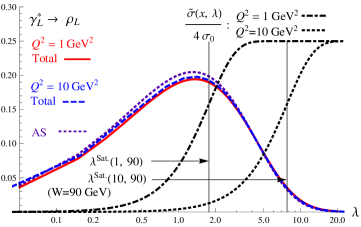
Figure 13: Full twist 3 (Total) $P_{00}(\lambda,\mu_{F}^{2}(Q^{2}))$ for $Q^{2}=1$GeV² (solid red) and $Q^{2}=10$GeV² (dashed blue), AS $P^{(AS)}_{00}(\lambda)$ (dotted purple) and $\tilde{\sigma}(x,\lambda)$ at $W=90\;$GeV² for $Q^{2}=1\;$GeV²(dotted-dashed black) and $Q^{2}=10\;$GeV² (dashed black).

In figure 13 we show the Total and AS rescaled radial distributions $P_{00}(\lambda,\mu_{F}^{2}(Q^{2}))$ and $P_{00}^{(AS)}(\lambda,\mu_{F}^{2}(Q^{2}))$. This last one reads

$$P_{00}^{(AS)}(\lambda)=\frac{1}{Q}\mathcal{P}_{00}^{(AS)}(\frac{\lambda}{Q},Q^{2})=6\,\int dy\,(y{\bar{y}})^{2}\lambda\,K_{0}(\sqrt{y{\bar{y}}}\lambda)\,.$$ (73)

The average value of $\lambda$ estimated with $P_{00}^{(AS)}(\lambda)$ is

$$\left\langle\lambda\right\rangle_{00}^{(AS)}=\int d\lambda\,\lambda\,P_{00}^{(AS)}(\lambda)=\frac{3\pi^{2}}{8}\approx 3.7\,.$$ (74)

About half of the dipoles are contained in the region $1<\lambda<\left\langle\lambda\right\rangle_{00}^{(AS)}\,,$ the peak of the distribution being at $\lambda^{\text{peak}}\sim 1.3$. The typical transverse scale $\mu=\sqrt{y{\bar{y}}\,Q^{2}}$ entering the wave functions overlap can be estimated using eq. (72),

$$\frac{\left\langle\mu\right\rangle_{00}^{(AS)}}{Q}=\left\langle\sqrt{y{\bar{y}}}\right\rangle^{(AS)}_{00}=6\,\int dy\,\int d\lambda\,(\sqrt{y{\bar{y}}})\,\left((y{\bar{y}})^{2}\lambda\,K_{0}(\sqrt{y{\bar{y}}}\lambda)\right)=\frac{9\pi}{64}\approx 0.44\,.$$ (75)

The choice of the factorization scale $\mu_{F}(Q^{2})$ given by eq. (55) is then a good approximation of the transverse dynamical scale $\left\langle\mu\right\rangle^{(AS)}_{00}$ involved in the process.

The dipole scattering amplitude plays the role of a filter that selects dipoles of $\lambda>\lambda^{\text{Sat.}}(Q^{2},W)=2R_{0}(x)\,Q$. Note that the critical saturation line eq. (42) is given by

$$\lambda^{\text{Sat.}}(Q_{S}^{2}(x(Q_{S}^{2},W^{2})),W)=2\,,$$ (76)

where

$$x(Q^{2},W^{2})=\frac{Q^{2}}{W^{2}+Q^{2}}\left(1+\frac{4\,m_{f}^{2}}{Q^{2}}\right)\,,$$ (77)

in accordance with eq. 43. In the kinematics of HERA, the energy in the center of mass $W$ varies roughly from $50\;$GeV to $150\;$GeV, leading to the following bounds for the two values $Q^{2}=1\;$GeV² and $Q^{2}=10\;$GeV²,

$$\lambda^{\text{Sat.}}(1,50) = 2.1>\lambda^{\text{Sat.}}(1,W)>\lambda^{\text{Sat.}}(1,150)=1.5$$ (78)

$$\lambda^{\text{Sat.}}(10,50) = 9.2>\lambda^{\text{Sat.}}(10,W)>\lambda^{\text{Sat.}}(10,150)=6.7\,.$$ (79)

We will fix for our purpose $W=90\;$GeV resulting in the values, ($\lambda^{\text{Sat.}}(1\;\text{GeV}^{2},90\;$GeV)$\sim 1.8$) and ($\lambda^{\text{Sat.}}(10\;\text{GeV}^{2},90\;$GeV)$\sim 7.7$). We can then differentiate the case $Q^{2}=1\;$GeV² where we are in the saturation regime ($\lambda^{\text{Sat.}}(1\;\text{GeV}^{2},90\;$GeV)$<2$), and the case $Q^{2}=10\;$GeV² where saturation effect are less important ($\lambda^{\text{Sat.}}(10\;\text{GeV}^{2},90\;$GeV)$>2$).

Figure 14: The normalized integrand of $T_{00}$, i.e. $\mathcal{P}_{00}(r,Q^{2},\mu_{F}^{2})\,\hat{\sigma}(x,r)$. The Total integrand at $\mu_{F}^{2}(Q^{2})$ for $Q^{2}=1\;$GeV²(blue long-dashed line) and $Q^{2}=10\;$GeV² (red solid line), and the AS integrand for $Q^{2}=1\;$GeV²(blue dot-dashed line) and $Q^{2}=10\;$GeV² (red dashed line) integrands of $T_{00}$ for $W=90\;$GeV.

We can evaluate the percentages $N_{\lambda>\lambda^{\text{Sat.}}}$ of the dipoles large enough to be in the bandwidth of the dipole cross-section, for each $Q^{2}$,

$$N_{\lambda>\lambda^{\text{Sat.}}}(Q^{2}=1\;\text{GeV}^{2},\,W=90\,\text{GeV}) = \int_{\lambda^{\text{Sat.}}(1,\,90)}^{\infty}d\lambda\,P^{(AS)}_{00}(\lambda)=70\%\,,$$ (80)

$$N_{\lambda>\lambda^{\text{Sat.}}}(Q^{2}=10\;\text{GeV}^{2},W=90\,\text{GeV}) = \int_{\lambda^{\text{Sat.}}(10,\,90)}^{\infty}d\lambda\,P^{(AS)}_{00}(\lambda)=10\%\,,$$ (81)

as one can see in figure 13 (plotted in logarithmic scale). The large difference between $N_{\lambda>\lambda^{\text{Sat.}}}(1,90)$ and $N_{\lambda>\lambda^{\text{Sat.}}}(10,90)$ indicates that the integrand of $T_{00}$ shown in figure 14, is very sensitive, when $Q^{2}$ varies between 1 GeV² and 10 GeV², to the overlapping of the dipole cross-section bandwidth ($\lambda>\lambda^{\text{Sat.}}(Q^{2},W)$) and the radial dipole distribution $P_{00}^{(AS)}(\lambda)$; we are then probing with a high accuracy the quality of the shape of the dipole cross-section.

At high $Q^{2}$ the tails of the distributions plays a dominant role. The tail of the distribution corresponds to the region where the integrand of the radial distribution can be approximated by an exponential fall,

$$\lambda\,K_{0}(\sqrt{y{\bar{y}}}\lambda)\xrightarrow[]{\lambda\gtrsim\lambda^{\text{tail}}}\sqrt{\lambda}\,exp(-\sqrt{y{\bar{y}}}\lambda)\,,$$ (82)

where typically

$$\lambda^{\text{tail}}\sim\frac{2}{\left\langle\sqrt{y{\bar{y}}}\,\right\rangle_{00}^{(AS)}}\approx 4.5\,.$$ (83)

In the case $Q^{2}=1\;$GeV², the bandwidth of the dipole cross-section mostly overlaps with the peak of the distributions as $\lambda^{\text{Sat.}}(1,90)\sim\lambda^{\text{peak}}$, while it only overlaps with the tail of the distribution when $Q^{2}=10\;$GeV², $\lambda^{\text{Sat.}}(10,90)\sim\lambda^{\text{tail}}$.

Figure 14 shows the normalized integrand of $T_{00}.$ This summarize our discussion on the respective role of the radial distribution and of the dipole cross-section. This integrand is peaked near the saturation radius $r\sim 2R_{0}(x)$. Comparing the cases $Q^{2}=10\;$GeV² and $Q^{2}=1\;$GeV², we see that this peak is moving to the right as $Q^{2}$ decreases, going through the bandwidth of the dipole cross-section.

6.2 The radial distribution of the $\gamma^{*}_{T}\to\rho_{T}$ transition

Figure 15: The Total $P_{11}(\lambda,\mu_{F}^{2}(Q^{2}))$ (red solid lines) results and their WW (blue dot-dashed lines) and genuine (Gen) (orange dashed lines) contributions, as well as the AS (purple long-dashed line) result $P^{(AS)}_{11}(\lambda)$ and the dipole cross-sections $\tilde{\sigma}(x,\lambda)$ (black dot-dot-dashed lines) at $W=90\;$GeV², for $Q^{2}=1\;$GeV² (thick lines) and $Q^{2}=10\;$GeV² (thin lines).

In figure 15 are shown respectively for $Q^{2}=1\;$GeV² and $Q^{2}=10\;$GeV²,

1. the full twist 3 (Total) rescaled radial distribution $P_{11}(\lambda,\mu_{F}^{2}(Q^{2}))$, where we distinguish the two following contributions,

   • the WW contribution $\tilde{P}^{WW}_{11}(\lambda,\mu_{F}^{2}(Q^{2}))$,

   • the genuine contribution $\tilde{P}^{\text{gen}}_{11}(\lambda,\mu_{F}^{2}(Q^{2}))$,

   such as $P_{11}(\lambda,\mu_{F}^{2})=\left|\tilde{P}^{WW}_{11}(\lambda,\mu_{F}^{2})+\tilde{P}^{gen}_{11}(\lambda,\mu_{F}^{2})\right|$,

2. the asymptotic rescaled radial distribution $P^{(AS)}_{11}(\lambda)$, using the asymptotic distribution amplitudes.

Contrary to the $\gamma^{*}_{L}\to\rho_{L}$ transition, we see that the dependence on $\mu_{F}^{2}$ is quite strong if one compares $P_{11}(\lambda,\mu_{F}^{2})$ to $P^{(AS)}_{11}(\lambda)$. We cannot then restrict ourselves to only study the asymptotic case.

It is interesting to estimate the average $\left\langle\lambda\right\rangle$ obtained with the different distributions $P_{11}$, $P^{(AS)}_{11}$, $P^{WW}_{11}$ and $P^{\text{gen}}_{11}$, where $P^{WW}_{11}$ and $P^{\text{gen}}_{11}$ have been normalized separately. The explicit expression for the asymptotic distribution

$$P^{(AS)}_{11}(\lambda)=\frac{1}{Q}\mathcal{P}^{(AS)}_{11}\left(\frac{\lambda}{Q},Q^{2}\right)=\frac{3}{4}\,\int dy\,(y{\bar{y}})^{3/2}(y^{2}+{\bar{y}}^{2})\,\lambda^{2}K_{1}(\sqrt{y{\bar{y}}}\lambda)\,,$$ (84)

leads to

$$\left\langle\lambda\right\rangle^{(AS)}_{11}=\int d\lambda\,\lambda\,P^{11,(AS)}(\lambda)=\frac{27\pi^{2}}{32}\approx 8.33\,.$$ (85)

The average value of $\lambda$ estimated with the WW distribution is,

$$\left\langle\lambda\right\rangle^{WW}_{11}(\mu_{F}^{2}) = \int d\lambda\,\lambda\,P^{11,\,WW}(\lambda,\mu_{F}^{2})$$ (86)

$$= \frac{\int d\lambda\,\lambda\int dy\,\left(y{\bar{y}}\varphi_{3}^{WW}(y,\mu_{F}^{2})\lambda K_{1}(\sqrt{y{\bar{y}}}\lambda)\right)}{\int d\lambda\int dy\,\left(y{\bar{y}}\varphi_{3}^{WW}(y,\mu_{F}^{2})\lambda K_{1}(\sqrt{y{\bar{y}}}\lambda)\right)}$$

$$= \frac{9\pi^{2}}{512}(48+13a_{2}^{\|}(\mu_{F}^{2}))\xrightarrow[]{\mu_{F}^{2}\to\infty}\left\langle\lambda\right\rangle^{(AS)}_{11}\,.$$

The effect of the term involving $a_{2}^{\|}(\mu_{F}^{2})$ in the r.h.s. of eq. (86) is under $4\%$, which indicates that $P^{WW}_{11}(\lambda,\mu_{F}^{2})\sim P^{AS}_{11}(\lambda,\mu_{F}^{2})$ is a good approximation. The computation of the average values of $\lambda$ for the all the different contributions are given in table 4.

	Total	WW	genuine	AS
$\left\langle\lambda\right\rangle_{11}(\mu_{F}^{2}(1\;\text{GeV}^{2}))$	6.3	8.7	3.2	8.3
$\left\langle\lambda\right\rangle_{11}(\mu_{F}^{2}(10\;\text{GeV}^{2}))$	7.3	8.5	3.5	8.3

Table 4: Average values of $\left\langle\lambda\right\rangle=\left\langle r\,Q\right\rangle$ for the different contributions to the radial distribution for two values of $\mu_{F}^{2}(Q^{2})$.

The results in table 4 show that the $\gamma^{*}_{T}\to\rho_{T}$ transition is more sensitive to saturation effects than the $\gamma^{*}_{L}\to\rho_{L}$ transition as $\left\langle\lambda\right\rangle_{11}$ is about twice larger than $\left\langle\lambda\right\rangle_{00}$. Indeed it means that more dipoles are produced in the bandwidth of the dipole cross-section by the radial distribution $P_{11}(\lambda,\mu_{F}^{2})$ than $P_{00}(\lambda,\mu_{F}^{2})$. As a consequence the polarized cross-section $\sigma_{T}$ should be a more sensitive observable to probe features of the saturation regime than $\sigma_{L}$.

The transverse dipole scale associated to the WW contribution, using eq. (72), is

$$\langle\mu\rangle^{WW}_{11}=Q\,\left\langle\sqrt{y{\bar{y}}}\right\rangle_{11}^{WW}\approx\frac{Q}{2.7}\,.$$

which is not so far from the values of the function $\mu_{F}^{2}(Q^{2})=\frac{Q^{2}+M_{\rho}^{2}}{4}$ that is used here.

The tail of the distribution $\tilde{P}^{WW}_{11}(\lambda,\mu_{F}^{2})$ can be defined as,

$$\lambda^{2}\,K_{1}(\sqrt{y{\bar{y}}}\lambda)\xrightarrow[]{\lambda>\lambda^{\text{tail}\,WW}}\lambda\,\sqrt{\lambda}\,\exp(-\sqrt{y{\bar{y}}}\lambda)\,,$$ (87)

where

$$\lambda^{\text{tail}\,WW}\sim\frac{4}{\left\langle\sqrt{y{\bar{y}}}\right\rangle_{11}^{WW}}\approx 10.9\,,$$ (88)

in which the average value $\left\langle\sqrt{y{\bar{y}}}\right\rangle_{11}^{WW}$ is approximated by $\left\langle\sqrt{y{\bar{y}}}\right\rangle_{11}^{AS}\approx 0.37$.

The genuine contribution $P^{\text{gen}}_{11}(\lambda,\mu_{F}^{2})$, which vanishes in the limit $\mu_{F}^{2}\to\infty$, depends strongly on the factorization scale $\mu_{F}^{2}(Q^{2})$, as one can see in figure 15. The distribution $P^{\text{gen}}_{11}(\lambda,\mu_{F}^{2})$ can be split into two contributions,

$$P^{\text{gen}}_{11}(\lambda,\mu_{F}^{2})=\tilde{P}^{\text{gen}\,(q{\bar{q}})}_{11}(\lambda,\mu_{F}^{2})+\tilde{P}^{\text{gen}\,(q{\bar{q}}g)}_{11}(\lambda,\mu_{F}^{2})\,,$$ (89)

where

$$\tilde{P}^{\text{gen}\,(q{\bar{q}})}_{11}(\lambda,\mu_{F}^{2}) = \frac{\lambda}{Q^{2}{\cal N}_{11}}\int dy\,\psi^{\gamma^{*}_{T}\to\rho_{T}\,\text{gen}}_{(q{\bar{q}})}(y,\lambda/Q;Q,\mu_{F}^{2})\,,$$ (90)

$$\tilde{P}^{\text{gen}\,(q{\bar{q}}g)}_{11}(\lambda,\mu_{F}^{2}) = \frac{\lambda}{Q^{2}{\cal N}_{11}}\int dy\int_{0}^{y}dy_{1}\,\psi^{\gamma^{*}_{T}\to\rho_{T}}_{(q{\bar{q}}g)}(y_{1},y,\lambda/Q;Q,\mu_{F}^{2})\,.$$ (91)

$\tilde{P}^{\text{gen}\,(q{\bar{q}})}_{11}(\lambda,\mu_{F}^{2})$ involves the exchange of two-parton in the hard part and the genuine solutions of the two-parton DAs, while $\mathcal{P}^{\text{gen}\,(q{\bar{q}}g)}_{11}(\lambda,\mu_{F}^{2})$ involves the three-parton exchange hard part $\mathcal{F}^{\gamma^{*}_{T}}(y_{1},y_{2},{\underline{r}};Q)$ defined in eq. (3.1).

The transverse scale $\mu$ present in $\tilde{P}^{\text{gen}\,(q{\bar{q}})}_{11}(\lambda,\mu_{F}^{2})$ is of order $\left\langle\sqrt{y{\bar{y}}}\right\rangle_{11}^{\text{gen}\,(q{\bar{q}})}(\mu_{F}^{2})\sim 0.5$ and is not very sensitive to $\mu_{F}^{2}$. The choice of $\mu_{F}^{2}(Q^{2})\sim\frac{Q}{2}$ is then a good choice for this contribution.

The contribution $\tilde{P}^{\text{gen}\,(q{\bar{q}}g)}_{11}(\lambda,\mu_{F}^{2})$ have several transverse scales which are $\mu_{1}$, $\mu_{2}$, $\mu_{{\bar{q}}g}$, $\mu_{qg}$ and $\mu_{q{\bar{q}}}$ defined by eqs. (25), each corresponding to a dipole configuration involving two of the three partons available in the process. In order to estimate these transverse scales, we first evaluate the average fraction of momentum carried by the quark $\left\langle y_{1}\right\rangle_{11}^{\text{gen}\,(q{\bar{q}}g)}(\mu_{F}^{2})$, the antiquark $\left\langle{\bar{y}}_{2}\right\rangle_{11}^{\text{gen}\,(q{\bar{q}}g)}(\mu_{F}^{2})$ and the gluon $\left\langle y_{g}\right\rangle_{11}^{\text{gen}\,(q{\bar{q}}g)}(\mu_{F}^{2})$, defined as

$$\left\langle y_{i}\right\rangle_{11}^{\text{gen}\,(q{\bar{q}}g)}(\mu_{F}^{2})=\frac{\displaystyle\int d\lambda\,\lambda\,\int dy_{2}\,\int_{0}^{y_{2}}dy_{1}\,y_{i}\,\psi^{\gamma^{*}_{T}\to\rho_{T}}_{(q{\bar{q}}g)}(y_{1},y_{2},{\underline{r}};Q,\mu_{F}^{2})}{\displaystyle\int d\lambda\,\lambda\,\int dy_{2}\,\int_{0}^{y_{2}}dy_{1}\,\psi^{\gamma^{*}_{T}\to\rho_{T}}_{(q{\bar{q}}g)}(y_{1},y_{2},{\underline{r}};Q,\mu_{F}^{2})}\,.\,$$ (92)

Using the fact that $\left\langle y_{1}\right\rangle_{11}^{\text{gen}\,(q{\bar{q}}g)}(\mu_{F}^{2})=\left\langle{\bar{y}}_{2}\right\rangle_{11}^{\text{gen}\,(q{\bar{q}}g)}(\mu_{F}^{2})$ due to the symmetry under the exchange of the quark and the antiquark, the obtained values are given in table 5.

$\left\langle y_{1}\right\rangle_{11}^{\text{gen}\,(q{\bar{q}}g)}(\mu_{F}^{2})$	$\left\langle{\bar{y}}_{2}\right\rangle_{11}^{\text{gen}\,(q{\bar{q}}g)}(\mu_{F}^{2})$	$\left\langle y_{g}\right\rangle_{11}^{\text{gen}\,(q{\bar{q}}g)}(\mu_{F}^{2})$
41.8%	41.8%	16.3%

Table 5: Average values $\left\langle y_{i}\right\rangle_{11}^{\text{gen}\,(q{\bar{q}}g)}(\mu_{F}^{2})$ of the fraction of longitudinal momentum of the $\rho$ meson carried by each of the parton $i$.

An estimation of the transverse scales can be made, using

$$\frac{\left\langle\mu_{1}\right\rangle}{Q}=\frac{\left\langle\mu_{2}\right\rangle}{Q} \sim \sqrt{\left\langle y_{1}\right\rangle(1-\left\langle y_{1}\right\rangle)}\approx 0.49\,,$$ (93)

$$\frac{\left\langle\mu_{qg}\right\rangle}{Q}=\frac{\left\langle\mu_{{\bar{q}}g}\right\rangle}{Q} \sim \sqrt{\frac{\left\langle y_{1}\right\rangle\,\left\langle y_{g}\right\rangle}{(1-\left\langle{\bar{y}}_{2}\right\rangle)}}\approx 0.34\,,$$ (94)

$$\frac{\left\langle\mu_{q{\bar{q}}}\right\rangle}{Q} \sim \sqrt{\frac{\left\langle y_{1}\right\rangle\,\left\langle{\bar{y}}_{2}\right\rangle}{(1-\left\langle y_{g}\right\rangle)}}\approx 0.46\,,$$ (95)

where we assume that the transverse scale values are roughly approximated by using the average fractions of longitudinal momentum in eqs. (25).

These values are evaluated at $\mu_{F}^{2}(1\;$GeV${}^{2})$. Other values of $\mu_{F}^{2}$ have also been used, leading to approximately the same results. We note that the function $\mu_{F}(Q^{2})\approx\frac{Q}{2}$ is close to the $\left\langle\mu_{1}\right\rangle$ and $\left\langle\mu_{q{\bar{q}}}\right\rangle$ values, and of the same order of magnitude than $\left\langle\mu_{qg}\right\rangle$ but in principle, one should adapt the choice of the factorization scale to the relevant transverse scales at stake for each part of the process.

The WW and the genuine contributions to the radial distribution $P_{11}(\lambda,\mu_{F}^{2})$ are of the same order of magnitude for $Q^{2}\sim 10\;$GeV², and the genuine contribution becomes even more important for $Q^{2}=1\;$GeV². At $Q^{2}=10\;$GeV², as

$$\left\langle\lambda\right\rangle_{11}^{\text{gen}}(\sim 3.5)\,<\,\lambda^{\text{Sat.}}(10\;\text{GeV}^{2})(\sim 7.7)\,<\,\left\langle\lambda\right\rangle^{WW}_{11}(\sim 8.7)\,,$$

most of the dipoles in the bandwidth of the dipole cross-section are provided by the WW contribution, which explains why the predictions for $\sigma_{T}$ are dominated by the WW predictions, as shown in figure 4(a), and consequently, why the results depend weakly on the factorization scale.

However the fact that the genuine contribution is important even at large $Q^{2}$, indicates that the three-parton exchange between the $\gamma^{*}_{T}$ and $\rho_{T}$ states is important in such relations as the normalization eq. (96) of the $\rho$ meson wave function [81, 7], and the electronic decay width eq. (97) [82, 7],

$$1 = \sum_{h,\tilde{h}}\int dy\int d^{2}{\underline{r}}\,\left|\Psi^{\rho_{T}}_{h,\tilde{h}}(y,{\underline{r}})\right|^{2}\,,$$ (96)

$$ef_{\rho}m_{\rho}(e^{*}_{\gamma}\cdot e_{\rho}) = \sum_{h,\tilde{h}}\int dy\int d^{2}{\underline{r}}\,\Psi^{\rho_{T}}_{h,\tilde{h}}(y,{\underline{r}})\,\Psi^{\gamma^{*}_{T}}_{h,\tilde{h}}(y,{\underline{r}})\,,$$ (97)

where the exchange of only two-parton is assumed. Indeed, the r.h.s. of eq. (97), if one expands at large $Q^{2}$ the $\rho$ meson wave function around ${\underline{r}}=0\,,$ is the WW approximated result, which therefore misses the genuine contributions arising from three-parton correlators, which can have a significant effect even for large $Q^{2}$ values, see figure 15. These relations are usually used to constrain the parameters of the wave function models of the $\rho$ meson, assuming that the meson is solely constituted of a quark and an antiquark, which then consist in neglecting the higher Fock state contributions like the genuine contribution. At $Q^{2}=1\;$GeV², the peak of the genuine part of the radial distribution enters the dipole cross-section bandwidth ($\lambda^{\text{Sat.}}(1,90)<\left\langle\lambda\right\rangle^{\text{gen}}_{11}$) and gives an important contribution to the integrand of $T_{11}$. When increasing $Q^{2}$, as shown in figure 16 where we display the product $\mathcal{P}_{11}(r,Q^{2},\mu_{F}^{2})\hat{\sigma}(x,r)$ for $Q^{2}=1\;$GeV² and $Q^{2}=10\;$GeV², we can note that the difference between the AS and the Total results is a consequence of the genuine contribution growing when $Q^{2}$ decreases. It is the convolution with the dipole cross-section which washes-out the effect of these genuine twist-3 contributions.

Figure 16: The Total contributions at $\mu_{F}^{2}(Q^{2})$ for $Q^{2}=1\;$GeV² (blue long-dashed line) and $Q^{2}=10\;$GeV² (red solid line), and the AS contributions for $Q^{2}=1\;$GeV² (blue dot-dashed line) and $Q^{2}=10\;$GeV² (red dashed line) to the normalized integrands of $T_{11}$, i.e. $\mathcal{P}_{11}(r,Q^{2},\mu_{F}^{2})\hat{\sigma}(x,r)$, for $W=90\;$GeV.

6.3 Comparison with the radial distributions obtained from models of the $\rho$ meson wave function.

It is instructive to compare shapes of the radial distributions $\mathcal{P}_{00}$ and $\mathcal{P}_{11}$ used in our analysis with those used in two other approaches which involve the overlap of the virtual photon wave functions and of the $\rho$ meson wave functions:

• the ”Boosted Gaussian” (BG) model [46],

• the ”Gaus-LC” model [55].

We use here the convention and the parameter values of ref.[47], which for completeness are shown in table 6.

Model	$N_{T}$	$R_{T}^{2}\;$GeV-2	$N_{L}$	$R_{L}^{2}\;$GeV-2	$f_{\rho}^{T}$
Gaus-LC	4.47	21.9	1.79	10.4	$f_{\rho}$
Boosted Gaussian	0.911	0.853	12.9	$R_{L}^{2}$	0.182

Table 6: Parameter of the ”Gaus-LC” and the ”Boosted Gaussian” models taken from ref.[47], for $M_{\rho}=0.776\;$GeV, $f_{\rho}=0.156\;$GeV, $m_{f}=0.14\;$GeV and with $f_{\rho}^{L}=f_{\rho}$ .

The scalar parts of the wave functions are given by,

$$\phi^{\text{Gauss-LC}}_{T}(y,r) = N_{T}\,(y\,{\bar{y}})^{2}\,e^{-\frac{r^{2}}{2R_{T}^{2}}}\,,$$ (98)

$$\phi^{\text{Gauss-LC}}_{L}(y,r) = N_{L}\,y\,{\bar{y}}\,e^{-\frac{r^{2}}{2R_{L}^{2}}}\,,$$ (99)

$$\phi^{\text{BG}}_{L,T}(y,r) = N_{L,T}\,y\,{\bar{y}}\,\exp\left(-\frac{m_{f}^{2}R_{L,T}^{2}}{8y{\bar{y}}}-\frac{2y{\bar{y}}r^{2}}{R_{L,T}^{2}}+\frac{m_{f}^{2}R_{L,T}^{2}}{2}\right)\,.$$ (100)

The overlaps with the virtual photon wave function are,

$$\sum_{h,\bar{h}}\Psi^{\rho_{T}*}_{h,\tilde{h}}(y,{\underline{r}})\Psi^{\gamma^{*}_{T}}_{h,\tilde{h}}(y,{\underline{r}}) \propto m_{f}^{2}K_{0}(\mu r)\phi_{T}(y,r)-(y^{2}+{\bar{y}}^{2})\mu K_{1}(\mu r)\partial_{r}\phi_{T}(y,r)\,,$$ (101)

$$\sum_{h,\bar{h}}\Psi^{\rho_{L}*}_{h,\tilde{h}}(y,{\underline{r}})\Psi^{\gamma^{*}_{L}}_{h,\tilde{h}}(y,{\underline{r}}) \propto y{\bar{y}}K_{0}(\mu r)\left(m_{\rho}\phi_{L}(y,r)+\delta\frac{m_{f}^{2}-\nabla_{r}^{2}}{m_{\rho}y{\bar{y}}}\phi_{L}(y,r)\right)\,,$$ (102)

with $\delta=0$ for the Gaus-LC model and $\delta=1$ for the BG model. The radial distributions thus read,

$$\mathcal{P}_{L,T}(r)=\frac{1}{\mathcal{N}_{L,T}}r\int dy\,\sum_{h,\bar{h}}\Psi^{\rho_{L,T}*}_{h,\tilde{h}}(y,{\underline{r}})\Psi^{\gamma^{*}_{L,T}}_{h,\tilde{h}}(y,{\underline{r}})\,,$$ (103)

where the factors $\mathcal{N}_{L,T}$ normalize the distributions $\mathcal{P}_{L,T}(r)$.

(a) $\gamma^{*}_{L}\to\rho_{L}$ radial distributions and $\hat{\sigma}$ at $Q^{2}=1\;$GeV².

(b) $\gamma^{*}_{L}\to\rho_{L}$ radial distributions and $\hat{\sigma}$ at $Q^{2}=10\;$GeV².

(c) $\gamma^{*}_{T}\to\rho_{T}$ radial distributions and $\hat{\sigma}$ at $Q^{2}=1\;$GeV².

(d) $\gamma^{*}_{T}\to\rho_{T}$ radial distributions and $\hat{\sigma}$ at $Q^{2}=10\;$GeV².

Figure 17: The Gauss-LC (green, long dashed), BG (blue, dot-dot-dashed), Total (red, solid) and AS (red, dashed) radial distributions for the $\gamma^{*}_{L}\to\rho_{L}$ transition (top) and for the $\gamma^{*}_{T}\to\rho_{T}$ transition (bottom), vs $r$ for $Q^{2}=1\;$GeV² (left) and $Q^{2}=10\;$GeV² (right), as well as the dipole cross-section $\hat{\sigma}(x,r)$ rescaled by the factor $5\sigma_{0}$ for $W=90\;$GeV (black, dot-dashed).

Comparing the distributions at $Q^{2}=1\;$GeV² (figures 17(a) and 17(c)) and $Q^{2}=10\;$GeV² (figures 17(b) and 17(d)) we see that at large $Q^{2}$, in the bandwidth of the dipole cross-section, our distributions are converging with the distributions obtained from the Gaus-LC and BG models.

In the $\gamma^{*}_{T}\to\rho_{T}$ case in figures 17(c) and 17(d), we see that the BG and Gaus-LC models are closer to the distribution $\mathcal{P}_{11}$ than to the asymptotic distribution. When compared to other distributions, the asymptotic distribution $\mathcal{P}_{11}^{AS}$ is shifted to the right, thus selecting larger dipole sizes.

In the $\gamma^{*}_{L}\to\rho_{L}$ case, in figure 17(a) we see that the distributions from the Gaus-LC and BG models are not close to our predictions, indicating that the higher twist corrections are presumably more important at small $Q^{2}$ than in the $\gamma^{*}_{T}\to\rho_{T}$ transition.

These qualitative remarks remains the same when using the AAMQS dipole models, and we expect that they are model independent.

7 Conclusions

We performed phenomenological analysis of experimental data from HERA on $\rho$ meson electroproduction within the approach based on the recently derived [44] impact parameter representation of $\gamma^{*}\to\rho$ impact factor up to twist-3 accuracy. The important feature of this representation consists in the inclusion of contributions coming from both two- and three-partonic Fock states, maintaining a close connection with the dipole model picture. Consequently, it was possible to include in our framework the saturation effects. Our predictions show that we can get simultaneously good predictions for the polarized cross-sections $\sigma_{T}$ and $\sigma_{L}$. The abilility of the model to reproduce the data is the confirmation of the following points:

• the factorization of the dipole cross-section in the helicity amplitudes of the electroproduction of the $\rho$ meson works and, as an universal quantity, is the same for $T_{00}$ and $T_{11}$, giving the good energy dependence and normalizations of the polarized cross-sections,

• the collinear factorization procedure of the $\rho$ meson is justified and works successfully beyond the leading twist.

As expected the model has some limits due to the truncation of the twist expansion. Thanks to HERA data, we have identified the virtuality $Q^{2\,{\rm min}}\sim 5\;$GeV² were the higher twist corrections become important, which is a motivation to compute impact factors beyond the twist 3 accuracy in order to probe the genuine saturation regime which starts at $Q_{S}^{2}\sim\leavevmode\nobreak\ \!\!1\,$GeV².

Other helicity amplitudes could be computed keeping the same approach, they would be useful in the $t\neq t_{\rm min}$ regime. The kinematics of the impact factor can be also extended to take into account the $t-$dependence of the impact factors, which would be a test for the dipole models which include the impact parameter dependence, providing a probe of the proton shape [7], in particular through local geometrical scaling [83, 84].

Data also exist for $\phi$ leptoproduction. In this case quark-mass effects should be taken into account, in particular, because this allows the transversely polarized $\phi$ to couple through its chiral-odd twist-2 DA. Indeed, as it was pointed out in [42], the fact that the ratio $T_{11}/T_{00}$ is not the same (after trivial mass rescaling) for $\rho$ and $\phi$ mesons points to the importance of this effect. This is also beyond the scope of our present study, but may open an interesting way for accessing chiral-odd DAs.

The next-to-leading order effects - both on the evolution and on the impact factor - should be studied, since it is now known that both may have a important phenomenological effect [85, 86, 87, 88, 89].

On the experimental side, the future Electron-Ion Collider [90] and Large Hadron Electron Collider [91] with a high center-of-mass energy and high luminosities, as well as the International Linear Collider [92, 93, 94] will hopefully open the opportunity to study in more detail the hard diffractive production of mesons [95, 96, 85, 97, 86, 98, 87, 99].

Appendix A Appendices

A.1 Distribution amplitudes in the LCCF parametrization

The seven chiral-even $\rho$-meson DAs up to twist 3 are defined through the following matrix elements of nonlocal light-cone operators [40], for two-parton

$$\left\langle\rho(p_{\rho})\left|\bar{\psi}(z)\gamma_{\mu}\psi(0)\right|0\right\rangle=m_{\rho}f_{\rho}\int^{1}_{0}dy\,e^{iyp.z}[\varphi_{1}(y;\mu_{F}^{2})(e^{*}.n)p_{\mu}+\varphi_{3}(y;\mu_{F}^{2})e_{T\mu}^{*}]\,,$$ (105)

$$\left\langle\rho(p_{\rho})\left|\bar{\psi}(z)\gamma_{5}\gamma_{\mu}\psi(0)\right|0\right\rangle=i\,m_{\rho}f_{\rho}\,R^{*}_{\perp\mu}\int^{1}_{0}dy\,e^{iyp.z}\varphi_{A}(y;\mu_{F}^{2})\,,$$

$$\left\langle\rho(p_{\rho})\right|\bar{\psi}(z)\gamma_{\mu}i\stackrel{{\scriptstyle\longleftrightarrow}}{{\partial^{T}_{\alpha}}}\psi(0)\left|0\right\rangle=m_{\rho}f_{\rho}\,p_{\mu}e^{*}_{T\alpha}\int^{1}_{0}dy\,e^{iyp.z}\varphi_{1}^{T}(y;\mu_{F}^{2})\,,$$ (107)

$$\left\langle\rho(p_{\rho})\right|\bar{\psi}(z)\gamma_{5}\gamma_{\mu}i\stackrel{{\scriptstyle\longleftrightarrow}}{{\partial^{T}_{\alpha}}}\psi(0)\left|0\right\rangle=i\,m_{\rho}f_{\rho}\,p_{\mu}\,R^{*}_{\perp\alpha}\int^{1}_{0}dy\,e^{iyp.z}\varphi_{A}^{T}(y;\mu_{F}^{2})\,,$$

and three-parton correlators

$$\left\langle\rho(p_{\rho})\left|\bar{\psi}(z_{1})\gamma_{\mu}gA^{T}_{\alpha}(z_{2})\psi(0)\right|0\right\rangle=m_{\rho}f^{V}_{3\rho}(\mu_{F}^{2})\,p_{\mu}\,e_{T\alpha}^{*}$$ (108)

$$\hskip 56.9055pt\times\int^{1}_{0}dy_{2}\int^{y_{2}}_{0}dy_{1}e^{iy_{1}p.z_{1}+i(y_{2}-y_{1})p.z_{2}}B(y_{1},y_{2};\mu_{F}^{2})$$

$$\left\langle\rho(p_{\rho})\left|\bar{\psi}(z_{1})\gamma_{5}\gamma_{\mu}gA^{T}_{\alpha}(z_{2})\psi(0)\right|0\right\rangle=i\,m_{\rho}f^{A}_{3\rho}(\mu_{F}^{2})\,p_{\mu}\,R^{*}_{\perp\alpha}$$ (109)

$$\hskip 56.9055pt\times\int^{1}_{0}\!\!\!\!dy_{2}\!\int^{y_{2}}_{0}\!\!\!\!dy_{1}\,e^{iy_{1}p.z_{1}+i(y_{2}-y_{1})p.z_{2}}D(y_{1},y_{2};\mu_{F}^{2})\,,\,\,$$

where we used the standard notation $\stackrel{{\scriptstyle\longleftrightarrow}}{{\partial_{\rho}}}=\frac{1}{2}(\stackrel{{\scriptstyle\longrightarrow}}{{\partial_{\rho}}}-\stackrel{{\scriptstyle\longleftarrow}}{{\partial_{\rho}}})\,.$

DAs are linked by linear differential relations derived from equations of motion and $n-$independency condition [39, 40]. The solutions for $\varphi_{P}(y)\equiv\{\varphi_{3},\varphi_{A},\varphi_{1}^{T},\varphi_{A}^{T}\}$ are the sum of the solutions in the so-called WW approximation and of genuine solutions,

$$\varphi_{P}(y)=\varphi^{WW}_{P}(y)+\varphi^{gen}_{P}(y)\,.$$ (110)

The WW approximation consists in neglecting the contribution from three-parton operators, thus taking $B(y_{1},y_{2};\mu_{F}^{2})=D(y_{1},y_{2};\mu_{F}^{2})=0$. Then, $\varphi_{P}^{WW}(y)$ become functions of $\varphi_{1}(y)$ only, and their explicit expressions are given by

$$\varphi^{WW}_{3}(y;\mu_{F}^{2}) = \frac{1}{2}\left[\int^{y}_{0}du\frac{\varphi_{1}(u;\mu_{F}^{2})}{\bar{u}}+\int^{1}_{y}du\frac{\varphi_{1}(u;\mu_{F}^{2})}{u}\right]\,,$$ (111)

$$\varphi^{WW}_{A}(y;\mu_{F}^{2}) = \frac{1}{2}\left[\int^{y}_{0}du\frac{\varphi_{1}(u;\mu_{F}^{2})}{\bar{u}}-\int^{1}_{y}du\frac{\varphi_{1}(u;\mu_{F}^{2})}{u}\right]\,,$$ (112)

$$\varphi^{T\,WW}_{A}(y;\mu_{F}^{2}) = -\frac{1}{2}\left[\bar{y}\int^{y}_{0}du\frac{\varphi_{1}(u;\mu_{F}^{2})}{\bar{u}}+y\int^{1}_{y}du\frac{\varphi_{1}(u;\mu_{F}^{2})}{u}\right]\,,$$ (113)

$$\varphi^{T\,WW}_{1}(y;\mu_{F}^{2}) = \frac{1}{2}\left[-\bar{y}\int^{y}_{0}du\frac{\varphi_{1}(u;\mu_{F}^{2})}{\bar{u}}+y\int^{1}_{y}du\frac{\varphi_{1}(u;\mu_{F}^{2})}{u}\right]\,.$$ (114)

Genuine solutions only depend on $\{B(y_{1},y_{2};\mu_{F}^{2}),D(y_{1},y_{2};\mu_{F}^{2})\}$ or equivalently on the combinations $\{S(y_{1},y_{2};\mu_{F}^{2}),M(y_{1},y_{2};\mu_{F}^{2})\}$ defined by eq. (3.1), namely

$$\varphi^{gen}_{3}(y;\mu_{F}^{2}) = \frac{1}{2}\left[\int^{1}_{\bar{y}}du\,\frac{A(u;\mu_{F}^{2})}{u}+\int^{1}_{y}du\,\frac{A(u;\mu_{F}^{2})}{u}\right]$$ (115)

$$\varphi^{gen}_{A}(y;\mu_{F}^{2}) = \frac{1}{2}\left[\int^{1}_{\bar{y}}du\,\frac{A(u;\mu_{F}^{2})}{u}-\int^{1}_{y}du\,\frac{A(u;\mu_{F}^{2})}{u}\right]\,,$$ (116)

where $A(u;\mu_{F}^{2})$ has the compact form

$$A(u;\mu_{F}^{2})=\int^{u}_{0}dy_{2}\left[\frac{1}{y_{2}-u}-\partial_{u}\right]M(y_{2},u;\mu_{F}^{2})+\int^{1}_{u}dy_{2}\frac{1}{y_{2}-u}M(u,y_{2};\mu_{F}^{2})$$ (117)

and it obeys the conditions

$$\int^{1}_{0}du\,A(u;\mu_{F}^{2})=0\quad{\rm and}\quad\int^{1}_{0}du\,\bar{u}\,A(u;\mu_{F}^{2})=0\,,$$ (118)

coming, respectively, from the constraints

$$\int^{1}_{0}\varphi_{3}^{gen}(y;\,\mu_{F}^{2})\,dy=0\quad{\rm and}\quad\int^{1}_{0}(y-\bar{y})\,\varphi_{A}^{gen}(y;\,\mu_{F}^{2})\,dy=0\,.$$ (119)

Equations (115) and (116) determine the expressions of $\varphi^{gen}_{1T}(y;\mu_{F}^{2})$ and $\varphi^{gen}_{AT}(y;\mu_{F}^{2})$ as

$$\varphi^{T\,gen}_{1}(y;\mu_{F}^{2}) = \int^{y}_{0}du\,\varphi^{gen}_{3}(u;\mu_{F}^{2})$$

$$-\frac{1}{2}\int^{y}_{0}dy_{1}\int^{1}_{y}dy_{2}\frac{S(y_{1},y_{2};\mu_{F}^{2})+M(y_{1},y_{2};\mu_{F}^{2})}{y_{2}-y_{1}}\,,$$

$$\varphi^{T\,gen}_{A}(y;\mu_{F}^{2}) = \int^{y}_{0}du\,\varphi^{gen}_{A}(u;\mu_{F}^{2})$$

$$-\frac{1}{2}\int^{y}_{0}dy_{1}\int^{1}_{y}dy_{2}\frac{S(y_{1},y_{2};\mu_{F}^{2})-M(y_{1},y_{2};\mu_{F}^{2})}{y_{2}-y_{1}}\,.$$

The correspondence between our set of DAs and the one defined in ref. [50] is achieved through the following dictionary derived in ref. [40]. It reads, for the two-parton vector DAs,

$$\varphi_{1}(y)=\phi_{\parallel}(y),\quad\varphi_{3}(y)=g_{\perp}^{(v)}(y)\,,$$ (122)

and for the axial DA,

$$\varphi_{A}(y)=-\frac{1}{4}\,\frac{\partial g_{\perp}^{(a)}(y)}{\partial y}\,.$$ (123)

For the three-parton DAs, the identification is

$$B(y_{1},\,y_{2})=-\frac{V(y_{1},\,1-y_{2})}{y_{2}-y_{1}}\quad{\rm and}\quad D(y_{1},\,y_{2})=-\frac{A(y_{1},\,1-y_{2})}{y_{2}-y_{1}}\,.$$ (124)

Explicit forms for $\varphi_{1}$, $B$, and $D$ are obtained with the help of the results of ref. [50] obtained within the QCD sum rules approach. The first terms of the expansion in the momentum fractions of the three independent DAs thus have the form

$$\varphi_{1}(y,\mu_{F}^{2}) = 6\,y\bar{y}\left[1+a_{2}^{\|}(\mu_{F}^{2})\frac{3}{2}(5(y-\bar{y})^{2}-1)\right]\,,$$ (125)

$$B(y_{1},y_{2};\mu_{F}^{2}) = -5040\,y_{1}\bar{y}_{2}(y_{1}-\bar{y}_{2})(y_{2}-y_{1})\,,$$ (126)

$$D(y_{1},y_{2};\mu_{F}^{2}) = -360\,y_{1}\bar{y}_{2}(y_{2}-y_{1})\left[1+\frac{\omega^{A}_{\{1,0\}}(\mu_{F}^{2})}{2}(7(y_{2}-y_{1})-3)\right]\,.$$ (127)

The dependences on the renormalization scale $\mu_{F}$ of the coupling constants $a_{2}^{\|}$, $\omega^{A}_{\{1,0\}}$, $\zeta^{A}_{3}$, and $\zeta^{V}_{3}$ are given in ref. [50]. In appendix A.2 we present both the evolution equations and the values of these constants at $\mu_{F}^{2}=1$ GeV² used in our analysis, as well as the dependence on $\mu_{F}$ of the DAs.

A.2 Evolutions of DAs and coupling constants with the renormalization scale

The parameters entering the DAs at $\mu_{0}^{2}=1\;$GeV² are updated in ref. [51] and their evolution equations are given in ref. [50], we recall in table 7 their values for the $\rho$ meson.

$\alpha_{s}$	0.52
$\omega^{A}_{\{1,0\}}$	-3.0
$\omega^{V}_{[0,1]}$	28/3
$a^{\|}_{2}$	0.15
$\zeta^{A}_{3}$	0.030
$\zeta^{V}_{3}$	0.011

Table 7: Coupling constants and Gegenbauer coefficients entering the $\rho$ meson DAs, at the scale $\mu_{0}=1$ GeV updated in ref. [51]. Note that in ref. [50] the normalization are such that $f^{V,A}_{3\rho\,\mbox{\cite[cite]{[\@@bibref{}{Ball:1998sk}{}{}]}}}=m_{\rho}\,f^{V,A}_{3\rho\,[{\rm here}]}$.

For $a_{2}^{\|}$, the evolution equation is

$$a_{2}^{\|}(\mu^{2})=a_{2}^{\|}(\mu_{0}^{2})\,L(\mu^{2})^{\gamma_{2}/b_{0}}$$ (128)

with

$$L(\mu^{2})=\frac{\alpha_{s}(\mu^{2})}{\alpha_{s}(\mu_{0}^{2})}=\frac{1}{1+\frac{b_{0}}{\pi}\alpha_{s}(\mu_{0}^{2})\ln(\mu^{2}/\mu_{0}^{2})}$$ (129)

where $b_{0}=(11N_{c}-2N_{f})/3\,,$ $\gamma_{n}=4C_{F}\left(\psi(n+2)+\gamma_{E}-\frac{3}{4}-\frac{1}{2(n+1)(n+2)}\right)$ and $\psi(n)=-\gamma_{E}+\sum^{n+1}_{k=1}1/k\,.$ For the $f^{A}_{3\rho}$ coupling constant, the evolution is given by

$$f^{A}_{3\rho}(\mu^{2})=f^{A}_{3\rho}(\mu_{0}^{2})\,L(\mu^{2})^{\Gamma^{-}_{2}/b_{0}}$$ (130)

with $\Gamma_{2}^{-}=-\frac{C_{F}}{3}+3\,C_{g}$ ($C_{g}=N_{c}$). The couplings $f^{V}_{3\rho}$ and $\omega^{A}_{\{0,1\}}(\mu^{2})f^{A}_{3\rho}(\mu^{2})$ enter a matrix evolution equation [50]. Defining

$$V(\mu^{2})=\left(\begin{array}[]{clrr}\omega^{V}_{[0,1]}f^{V}_{3\rho}(\mu^{2})-\omega^{A}_{\{0,1\}}(\mu^{2})f^{A}_{3\rho}(\mu^{2})\\ \\ \omega^{V}_{[0,1]}f^{V}_{3\rho}(\mu^{2})+\omega^{A}_{\{0,1\}}(\mu^{2})f^{A}_{3\rho}(\mu^{2})\end{array}\right)\,,$$ (134)

it reads

$$V(\mu^{2})=L(\mu^{2})^{\Gamma^{+}_{3}/b_{0}}V(1)\,,$$ (135)

with $\Gamma^{+}_{3}$ given by

$$\Gamma^{+}_{3}=\left(\begin{array}[]{clrr}\frac{8}{3}C_{F}+\frac{7}{3}C_{g}&\ \frac{2}{3}C_{F}-\frac{2}{3}C_{g}\\ \\ \frac{5}{3}C_{F}-\frac{4}{3}C_{g}&\ \frac{1}{6}C_{F}+4C_{g}\end{array}\right)\,.$$ (136)

Hence we get the dependence of $f^{V}_{3\rho}$ and $\omega^{A}_{\{0,1\}}$ by diagonalizing the system. The dependence of the DAs on the renormalization scale is shown in ref. [42]. The DAs exhibit a non-negligible effect of QCD evolution, in particular, for the genuine twist-3 contributions. We recall that we chose the collinear factorization scale of production of the $\rho$ meson $\mu_{F}$ to be equal to the renormalization scale of the process $\mu$, thus the dependence of the coupling constant in $\mu_{F}$ is given by eqs. (128, 130, 135).

A.3 Dipole-proton scattering amplitude in the GS-Model

In this appendix we calculate the Fourier transform of the proton impact factor. We denote by $r=\left|{\underline{r}}\right|$ the transverse size of the dipole. We should thus compute

$$\sigma(r)=A\int d^{2}{\underline{k}}\frac{1}{({\underline{k}}^{2})^{2}}\left(\frac{1}{M^{2}}-\frac{1}{M^{2}+{\underline{k}}^{2}}\right)(1-e^{i{\underline{k}}\cdot{\underline{r}}})(1-e^{-i{\underline{k}}\cdot{\underline{r}}})\,.$$ (137)

Using the notation $k=|{\underline{k}}|\,,$ the angular integration leads to

$$\sigma(r)=4\pi\,A\int dk\frac{1}{k^{3}}\left(\frac{1}{M^{2}}-\frac{1}{M^{2}+{\underline{k}}^{2}}\right)(1-J_{0}(k\,r))\,.$$ (138)

Relying on the identity

$$\frac{1}{k^{3}}\left(\frac{1}{M^{2}}-\frac{1}{M^{2}+k^{2}}\right)=\frac{1}{M^{4}}\left(\frac{1}{k}-\frac{k}{M^{2}+k^{2}}\right)\,,$$ (139)

we rewrite $\sigma(r)$ as

$$\sigma(r)=\frac{4\pi A}{M^{4}}I$$ (140)

with

$$I = \int^{\infty}_{0}\frac{dk}{k}-\int^{\infty}_{0}\frac{dk}{k}J_{0}(k\,r)-\int^{\infty}_{0}\frac{k}{M^{2}+k^{2}}dk+\int^{\infty}_{0}\frac{k}{M^{2}+k^{2}}J_{0}(k\,r)\,dk$$ (141)

$$= I_{1}-I_{2}-I_{3}+I_{4}\,.$$

The integral $I_{4}$ is UV and IR finite and reads [102]

$$I_{4}=K_{0}(M\,r)\,.$$ (142)

The integrals $I_{1}$ and $I_{2}$ are both IR divergent and are regularized through dimensional regularization, while the UV divergencies of $I_{1}$ and $I_{3}$ are regularized through a cut-off $\Lambda\,.$ We thus write

$$I_{1}=\int^{\Lambda}_{0}\frac{dk}{k^{1-\epsilon}}\sim\frac{1}{\epsilon}+\ln\Lambda\,.$$ (143)

Using the relation [102]

$$\int^{\infty}_{0}x^{\mu}\,J_{\nu}(a\,x)\,dx=2^{\mu}a^{-\mu-1}\frac{\Gamma\left(\frac{1}{2}+\frac{1}{2}\nu+\frac{1}{2}\mu\right)}{\Gamma\left(\frac{1}{2}+\frac{1}{2}\nu-\frac{1}{2}\mu\right)}$$ (144)

we obtain

$$I_{2}=\int^{\infty}_{0}\frac{dk}{k^{1-\epsilon}}J_{0}(k\,r)=2^{-1+\epsilon}\,r^{-\epsilon}\frac{\Gamma\left(\frac{\epsilon}{2}\right)}{\Gamma\left(1-\frac{\epsilon}{2}\right)}\sim\frac{1}{\epsilon}-\ln r-\gamma+\ln 2\,.$$ (145)

Finally,

$$I_{3}=\int^{\Lambda}_{0}\frac{k}{M^{2}+k^{2}}dk\sim\ln\Lambda-\ln M\,.$$ (146)

Thus, combining eqs. (143, 145, 146, 142) we get

$$I=\left(\gamma+\ln\frac{M\,r}{2}+K_{0}(M\,r)\right)\,,$$ (147)

and thus

$$\sigma(r)=\frac{4\pi\,A}{M^{4}}\left(\gamma+\ln\frac{M\,r}{2}+K_{0}(M\,r)\right)\,.$$ (148)

A.4 Results using the GBW and AAMQSb models

We present some of the predictions obtained by using the GBW or the AAMQSb model for the dipole cross-section. As expected the results are not so far from the ones obtained with the AAMQSa model. In figure 18 and 19 are respectively shown for the AAMQSb and the GBW model, the polarized cross-sections $\sigma_{T}$ and $\sigma_{T}$. The spin density matrix element $r^{04}_{00}$ predictions using these dipole models are shown in figure 20, for completeness we show also the prediction obtained with the GS model.

(a) $\sigma_{T}$ vs H1 data [4].

(b) $\sigma_{L}$ vs H1 data [4].

Figure 18: AS (purple dashed lines), WW (blue long dashed lines) and Total (red solid lines) contributions to $\sigma_{T}$ and $\sigma_{L}$ vs $Q^{2}$, for $W=75\;$GeV, using the AAMQSb-model, compared to the data of H1[4].

(a) $\sigma_{T}$ vs H1 data [4].

(b) $\sigma_{L}$ vs H1 data [4].

Figure 19: AS (purple dashed lines), WW (blue long dashed lines) and Total (red solid lines) contributions to $\sigma_{T}$ and $\sigma_{L}$ vs $Q^{2}$, for $W=75\;$GeV, using the GBW-model, compared to the data of H1[4].

(a) $r^{04}_{00}$ contributions using AAMQSb-model vs H1 data.

(b) $r^{04}_{00}$ contributions using AAMQSb-model vs ZEUS data.

(c) $r^{04}_{00}$ contributions using GBW-model vs H1 data.

(d) $r^{04}_{00}$ contributions using GBW-model vs ZEUS data.

(e) $r^{04}_{00}$ contributions using GS-model vs H1 data.

(f) $r^{04}_{00}$ contributions using GS-model vs ZEUS data.

Figure 20: Predictions for $r^{04}_{00}$ vs $W$ and $Q^{2}$ compared respectively with H1[4] and ZEUS[3] data, the AS (purple dashed lines), WW (blue long dashed lines), Total (red solid lines) contributions are shown separately using the AAMQSb-model, the GBW-model or the GS-model.

References

• [1] ZEUS Collaboration, J. Breitweg et. al., Exclusive electroproduction of $\rho^{0}$ and ${J}/\psi$ mesons at HERA, Eur. Phys. J. C6 (1999) 603–627, [hep-ex/9808020].
• [2] ZEUS Collaboration, J. Breitweg et. al., Measurement of the spin-density matrix elements in exclusive electroproduction of $\rho^{0}$ mesons at HERA, Eur. Phys. J. C12 (2000) 393–410, [hep-ex/9908026].
• [3] ZEUS Collaboration, S. Chekanov et. al., Exclusive $\rho^{0}$ production in deep inelastic scattering at HERA, PMC Phys. A1 (2007) 6, [arXiv:0708.1478].
• [4] H1 Collaboration, F. D. Aaron et. al., Diffractive Electroproduction of $\rho$ and $\phi$ Mesons at HERA, JHEP 05 (2010) 032, [arXiv:0910.5831].
• [5] A. Donnachie and P. Landshoff, Exclusive $\rho$ Production in Deep Inelastic Scattering, Phys.Lett. B185 (1987) 403.
• [6] J. Nemchik, N. N. Nikolaev, E. Predazzi, and B. Zakharov, Color dipole systematics of diffractive photoproduction and electroproduction of vector mesons, Phys.Lett. B374 (1996) 199–204, [hep-ph/9604419].
• [7] S. Munier, A. M. Stasto, and A. H. Mueller, Impact parameter dependent S-matrix for dipole proton scattering from diffractive meson electroproduction, Nucl. Phys. B603 (2001) 427–445, [hep-ph/0102291].
• [8] H. Cheng and T. T. Wu, Photon-photon scattering close to the forward direction, Phys. Rev. D1 (1970) 3414–3415.
• [9] G. Frolov and L. Lipatov Sov. J. Nucl. Phys. 13 (1971) 333.
• [10] V. Gribov, L. Lipatov, and G. Frolov, The leading singularity in the j plane in quantum electrodynamics, Sov.J.Nucl.Phys. 12 (1971) 543.
• [11] S. Catani, M. Ciafaloni, and F. Hautmann, Gluon contributions to small x heavy flavor production, Phys. Lett. B242 (1990) 97.
• [12] S. Catani, M. Ciafaloni, and F. Hautmann, High-energy factorization and small x heavy flavor production, Nucl. Phys. B366 (1991) 135–188.
• [13] J. C. Collins and R. K. Ellis, Heavy quark production in very high-energy hadron collisions, Nucl. Phys. B360 (1991) 3–30.
• [14] E. M. Levin, M. G. Ryskin, Y. M. Shabelski, and A. G. Shuvaev, Heavy quark production in semihard nucleon interactions, Sov. J. Nucl. Phys. 53 (1991) 657.
• [15] V. S. Fadin, E. A. Kuraev, and L. N. Lipatov, On the Pomeranchuk Singularity in Asymptotically Free Theories, Phys. Lett. B60 (1975) 50–52.
• [16] E. A. Kuraev, L. N. Lipatov, and V. S. Fadin, Multi - Reggeon Processes in the Yang-Mills Theory, Sov. Phys. JETP 44 (1976) 443–450.
• [17] E. A. Kuraev, L. N. Lipatov, and V. S. Fadin, The Pomeranchuk Singularity in Nonabelian Gauge Theories, Sov. Phys. JETP 45 (1977) 199–204.
• [18] I. I. Balitsky and L. N. Lipatov, The Pomeranchuk Singularity in Quantum Chromodynamics, Sov. J. Nucl. Phys. 28 (1978) 822–829.
• [19] V. S. Fadin, R. Fiore, and M. I. Kotsky, Gluon Regge trajectory in the two-loop approximation, Phys. Lett. B387 (1996) 593–602, [hep-ph/9605357].
• [20] G. Camici and M. Ciafaloni, Irreducible part of the next-to-leading BFKL kernel, Phys. Lett. B412 (1997) 396–406, [hep-ph/9707390].
• [21] M. Ciafaloni and G. Camici, Energy scale(s) and next-to-leading BFKL equation, Phys. Lett. B430 (1998) 349–354, [hep-ph/9803389].
• [22] V. S. Fadin and L. N. Lipatov, BFKL pomeron in the next-to-leading approximation, Phys. Lett. B429 (1998) 127–134, [hep-ph/9802290].
• [23] A. H. Mueller, Small x Behavior and Parton Saturation: A QCD Model, Nucl. Phys. B335 (1990) 115.
• [24] N. N. Nikolaev and B. G. Zakharov, Colour transparency and scaling properties of nuclear shadowing in deep inelastic scattering, Z. Phys. C49 (1991) 607–618.
• [25] S. J. Brodsky, L. Frankfurt, J. F. Gunion, A. H. Mueller, and M. Strikman, Diffractive leptoproduction of vector mesons in QCD, Phys. Rev. D50 (1994) 3134–3144, [hep-ph/9402283].
• [26] L. Frankfurt, W. Koepf, and M. Strikman, Hard diffractive electroproduction of vector mesons in QCD, Phys. Rev. D54 (1996) 3194–3215, [hep-ph/9509311].
• [27] J. C. Collins, L. Frankfurt, and M. Strikman, Factorization for hard exclusive electroproduction of mesons in QCD, Phys. Rev. D56 (1997) 2982–3006, [hep-ph/9611433].
• [28] A. V. Radyushkin, Nonforward parton distributions, Phys. Rev. D56 (1997) 5524–5557, [hep-ph/9704207].
• [29] G. R. Farrar and D. R. Jackson, The Pion Form-Factor, Phys. Rev. Lett. 43 (1979) 246.
• [30] G. P. Lepage and S. J. Brodsky, Exclusive Processes in Quantum Chromodynamics: Evolution Equations for Hadronic Wave Functions and the Form-Factors of Mesons, Phys. Lett. B87 (1979) 359–365.
• [31] A. V. Efremov and A. V. Radyushkin, Factorization and Asymptotical Behavior of Pion Form-Factor in QCD, Phys. Lett. B94 (1980) 245–250.
• [32] D. Yu. Ivanov, L. Szymanowski, and G. Krasnikov, Vector meson electroproduction at next-to-leading order, JETP Lett. 80 (2004) 226–230, [hep-ph/0407207].
• [33] H.-N. Li and G. Sterman, The Perturbative pion form-factor with Sudakov suppression, Nucl. Phys. B381 (1992) 129–140.
• [34] M. Vanderhaeghen, P. A. M. Guichon, and M. Guidal, Deeply virtual electroproduction of photons and mesons on the nucleon: Leading order amplitudes and power corrections, Phys. Rev. D60 (1999) 094017, [hep-ph/9905372].
• [35] S. V. Goloskokov and P. Kroll, Vector meson electroproduction at small Bjorken-x and generalized parton distributions, Eur. Phys. J. C42 (2005) 281–301, [hep-ph/0501242].
• [36] S. V. Goloskokov and P. Kroll, The longitudinal cross section of vector meson electroproduction, Eur. Phys. J. C50 (2007) 829–842, [hep-ph/0611290].
• [37] S. V. Goloskokov and P. Kroll, The role of the quark and gluon GPDs in hard vector-meson electroproduction, Eur. Phys. J. C53 (2008) 367–384, [/08.3569].
• [38] D. Yu. Ivanov and R. Kirschner, Polarization in diffractive electroproduction of light vector mesons, Phys. Rev. D58 (1998) 114026, [hep-ph/9807324].
• [39] I. V. Anikin, D. Yu. Ivanov, B. Pire, L. Szymanowski, and S. Wallon, On the description of exclusive processes beyond the leading twist approximation, Phys. Lett. B682 (2010) 413–418, [arXiv:0903.4797].
• [40] I. V. Anikin, D. Yu. Ivanov, B. Pire, L. Szymanowski, and S. Wallon, QCD factorization of exclusive processes beyond leading twist: $\gamma^{*}_{T}\to\rho_{T}$ impact factor with twist three accuracy, Nucl. Phys. B828 (2010) 1–68, [arXiv:0909.4090].
• [41] I. F. Ginzburg, S. L. Panfil, and V. G. Serbo, Possibility of the experimental investigation of the QCD Pomeron in semihard processes at the gamma gamma collisions, Nucl. Phys. B284 (1987) 685–705.
• [42] I. V. Anikin, A. Besse, D. Yu. Ivanov, B. Pire, L. Szymanowski, and S. Wallon, A phenomenological study of helicity amplitudes of high energy exclusive leptoproduction of the $\rho$ meson, Phys. Rev. D84 (2011) 054004, [arXiv:1105.1761].
• [43] J. F. Gunion and D. E. Soper, Quark Counting and Hadron Size Effects for Total Cross- Sections, Phys. Rev. D15 (1977) 2617–2621.
• [44] A. Besse, L. Szymanowski, and S. Wallon, The dipole representation of vector meson electroproduction beyond leading twist, Nucl. Phys. B867 (2013) 19–60, [arXiv:1204.2281].
• [45] J. Nemchik, N. N. Nikolaev, E. Predazzi, and B. G. Zakharov, Color dipole phenomenology of diffractive electroproduction of light vector mesons at HERA, Z. Phys. C75 (1997) 71–87, [hep-ph/9605231].
• [46] J. R. Forshaw, R. Sandapen, and G. Shaw, Colour dipoles and $\rho$, $\Phi$ electroproduction, Phys. Rev. D69 (2004) 094013, [hep-ph/0312172].
• [47] H. Kowalski, L. Motyka, and G. Watt, Exclusive diffractive processes at HERA within the dipole picture, Phys.Rev. D74 (2006) 074016, [hep-ph/0606272].
• [48] J. R. Forshaw and R. Sandapen, Extracting the $\rho$ meson wavefunction from HERA data, JHEP 11 (2010) 037, [arXiv:1007.1990].
• [49] J. Forshaw and R. Sandapen, Extracting the Distribution Amplitudes of the $\rho$ meson from the Color Glass Condensate, JHEP 1110 (2011) 093, [arXiv:1104.4753].
• [50] P. Ball, V. M. Braun, Y. Koike, and K. Tanaka, Higher twist distribution amplitudes of vector mesons in QCD: Formalism and twist three distributions, Nucl. Phys. B529 (1998) 323–382, [hep-ph/9802299].
• [51] P. Ball, V. Braun, and A. Lenz, Twist-4 distribution amplitudes of the $K^{*}$ and $\phi$ mesons in QCD, JHEP 0708 (2007) 090, [arXiv:0707.1201].
• [52] K. J. Golec-Biernat and M. Wusthoff, Saturation effects in deep inelastic scattering at low ${Q}^{2}$ and its implications on diffraction, Phys. Rev. D59 (1999) 014017, [hep-ph/9807513].
• [53] J. L. Albacete and Y. V. Kovchegov, Solving high energy evolution equation including running coupling corrections, Phys.Rev. D75 (2007) 125021, [arXiv:0704.0612].
• [54] J. L. Albacete, Particle multiplicities in Lead-Lead collisions at the LHC from non-linear evolution with running coupling, Phys.Rev.Lett. 99 (2007) 262301, [arXiv:0707.2545].
• [55] H. Kowalski and D. Teaney, An Impact parameter dipole saturation model, Phys.Rev. D68 (2003) 114005, [hep-ph/0304189].
• [56] J. R. Forshaw and D. A. Ross, Quantum chromodynamics and the pomeron, Cambridge Lect. Notes Phys. 9 (1997) 1–248.
• [57] G. Frolov, V. Gribov, and L. Lipatov, On Regge poles in quantum electrodynamics, Phys.Lett. B31 (1970) 34.
• [58] V. S. Fadin and A. D. Martin, Infrared safety of impact factors for colorless particle interactions, Phys. Rev. D60 (1999) 114008, [hep-ph/9904505].
• [59] The HERMES Collaboration, A. Airapetian et. al., Ratios of Helicity Amplitudes for Exclusive $\rho^{0}$ Electroproduction, Eur. Phys. J. C71 (2011) 1609, [arXiv:1012.3676].
• [60] A. G. Shuvaev, K. J. Golec-Biernat, A. D. Martin, and M. G. Ryskin, Off-diagonal distributions fixed by diagonal partons at small $x$ and $\xi$, Phys. Rev. D60 (1999) 014015, [hep-ph/9902410].
• [61] A. D. Martin, M. G. Ryskin, and T. Teubner, $Q^{2}$ dependence of diffractive vector meson electroproduction, Phys. Rev. D62 (2000) 014022, [hep-ph/9912551].
• [62] K. J. Golec-Biernat and M. Wusthoff, Saturation in diffractive deep inelastic scattering, Phys. Rev. D60 (1999) 114023, [hep-ph/9903358].
• [63] E. Gotsman, E. Levin, M. Lublinsky, and U. Maor, Towards a new global QCD analysis: Low x DIS data from nonlinear evolution, Eur.Phys.J. C27 (2003) 411–425, [hep-ph/0209074].
• [64] J. Bartels, K. J. Golec-Biernat, and H. Kowalski, A modification of the saturation model: DGLAP evolution, Phys. Rev. D66 (2002) 014001, [hep-ph/0203258].
• [65] E. Iancu, K. Itakura, and S. Munier, Saturation and BFKL dynamics in the HERA data at small x, Phys. Lett. B590 (2004) 199–208, [hep-ph/0310338].
• [66] J. L. Albacete, N. Armesto, J. G. Milhano, C. A. Salgado, and U. A. Wiedemann, Nuclear size and rapidity dependence of the saturation scale from QCD evolution and experimental data, Eur.Phys.J. C43 (2005) 353–360, [hep-ph/0502167].
• [67] V. Goncalves, M. Kugeratski, M. Machado, and F. Navarra, Saturation physics at HERA and RHIC: An Unified description, Phys.Lett. B643 (2006) 273–278, [hep-ph/0608063].
• [68] J. Jalilian-Marian, A. Kovner, A. Leonidov, and H. Weigert, The Wilson renormalization group for low x physics: Towards the high density regime, Phys. Rev. D59 (1999) 014014, [hep-ph/9706377].
• [69] J. Jalilian-Marian, A. Kovner, and H. Weigert, The Wilson renormalization group for low x physics: Gluon evolution at finite parton density, Phys. Rev. D59 (1999) 014015, [hep-ph/9709432].
• [70] A. Kovner, J. G. Milhano, and H. Weigert, Relating different approaches to nonlinear QCD evolution at finite gluon density, Phys. Rev. D62 (2000) 114005, [hep-ph/0004014].
• [71] H. Weigert, Unitarity at small Bjorken x, Nucl. Phys. A703 (2002) 823–860, [hep-ph/0004044].
• [72] E. Iancu, A. Leonidov, and L. D. McLerran, Nonlinear gluon evolution in the color glass condensate. I, Nucl. Phys. A692 (2001) 583–645, [hep-ph/0011241].
• [73] E. Ferreiro, E. Iancu, A. Leonidov, and L. McLerran, Nonlinear gluon evolution in the color glass condensate. II, Nucl. Phys. A703 (2002) 489–538, [hep-ph/0109115].
• [74] I. Balitsky, Operator expansion for high-energy scattering, Nucl. Phys. B463 (1996) 99–160, [hep-ph/9509348].
• [75] Y. V. Kovchegov, Small-$x$ $F_{2}$ structure function of a nucleus including multiple pomeron exchanges, Phys. Rev. D60 (1999) 034008, [hep-ph/9901281].
• [76] J. L. Albacete, N. Armesto, J. G. Milhano, and C. A. Salgado, Non-linear QCD meets data: A Global analysis of lepton-proton scattering with running coupling BK evolution, Phys.Rev. D80 (2009) 034031, [arXiv:0902.1112].
• [77] J. L. Albacete, N. Armesto, J. G. Milhano, P. Quiroga-Arias, and C. A. Salgado, AAMQS: A non-linear QCD analysis of new HERA data at small-x including heavy quarks, Eur.Phys.J. C71 (2011) 1705, [arXiv:1012.4408].
• [78] L. D. McLerran and R. Venugopalan, Boost covariant gluon distributions in large nuclei, Phys.Lett. B424 (1998) 15–24, [nucl-th/9705055].
• [79] A. H. Mueller, Soft gluons in the infinite momentum wave function and the BFKL pomeron, Nucl. Phys. B415 (1994) 373–385.
• [80] H. Navelet, R. B. Peschanski, C. Royon, and S. Wallon, Proton structure functions in the dipole picture of BFKL dynamics, Phys. Lett. B385 (1996) 357–364, [hep-ph/9605389].
• [81] G. P. Lepage and S. J. Brodsky, Exclusive Processes in Perturbative Quantum Chromodynamics, Phys. Rev. D22 (1980) 2157.
• [82] H. G. Dosch, T. Gousset, G. Kulzinger, and H. J. Pirner, Vector meson leptoproduction and nonperturbative gluon fluctuations in QCD, Phys. Rev. D55 (1997) 2602–2615, [hep-ph/9608203].
• [83] E. Ferreiro, E. Iancu, K. Itakura, and L. McLerran, Froissart bound from gluon saturation, Nucl.Phys. A710 (2002) 373–414, [hep-ph/0206241].
• [84] S. Munier and S. Wallon, Geometric scaling in exclusive processes, Eur. Phys. J. C30 (2003) 359–365, [hep-ph/0303211].
• [85] D. Yu. Ivanov and A. Papa, Electroproduction of two light vector mesons in the next- to-leading approximation, Nucl. Phys. B732 (2006) 183–199, [hep-ph/0508162].
• [86] D. Yu. Ivanov and A. Papa, Electroproduction of two light vector mesons in next-to-leading BFKL: Study of systematic effects, Eur. Phys. J. C49 (2007) 947–955, [hep-ph/0610042].
• [87] F. Caporale, A. Papa, and A. S. Vera, Collinear improvement of the BFKL kernel in the electroproduction of two light vector mesons, Eur. Phys. J. C53 (2008) 525–532, [arXiv:0807.0525].
• [88] D. Colferai, F. Schwennsen, L. Szymanowski, and S. Wallon, Mueller Navelet jets at LHC - complete NLL BFKL calculation, JHEP 12 (2010) 026, [arXiv:1002.1365].
• [89] B. Ducloué, L. Szymanowski, and S. Wallon, Mueller-Navelet jets at LHC: the first complete NLL BFKL study, PoS QNP2012 (2012) 165, [arXiv:1208.6111].
• [90] D. Boer, M. Diehl, R. Milner, R. Venugopalan, W. Vogelsang, et. al., Gluons and the quark sea at high energies: Distributions, polarization, tomography, arXiv:1108.1713.
• [91] LHeC Study Group Collaboration, J. Abelleira Fernandez et. al., A Large Hadron Electron Collider at CERN: Report on the Physics and Design Concepts for Machine and Detector, J.Phys. G39 (2012) 075001, [arXiv:1206.2913].
• [92] ILC Collaboration, J. Brau, (Ed. ) et. al., ILC Reference Design Report Volume 1 - Executive Summary, arXiv:0712.1950.
• [93] ILC Collaboration, G. Aarons et. al., International Linear Collider Reference Design Report Volume 2: PHYSICS AT THE ILC, arXiv:0709.1893.
• [94] ILC Collaboration, T. Behnke, (Ed. ) et. al., ILC Reference Design Report Volume 4 - Detectors, arXiv:0712.2356.
• [95] B. Pire, L. Szymanowski, and S. Wallon, Double diffractive $\rho$-production in $\gamma^{*}\gamma^{*}$ collisions, Eur. Phys. J. C44 (2005) 545–558, [hep-ph/0507038].
• [96] R. Enberg, B. Pire, L. Szymanowski, and S. Wallon, BFKL resummation effects in $\gamma^{*}\gamma^{*}\to\rho\rho$, Eur. Phys. J. C45 (2006) 759–769, [hep-ph/0508134].
• [97] B. Pire, M. Segond, L. Szymanowski, and S. Wallon, QCD factorizations in $\gamma^{*}\gamma^{*}\to\rho^{0}_{L}\rho^{0}_{L}$, Phys. Lett. B639 (2006) 642–651, [hep-ph/0605320].
• [98] M. Segond, L. Szymanowski, and S. Wallon, Diffractive production of two $\rho^{0}_{L}$ mesons in $e^{+}e^{-}$ collisions, Eur. Phys. J. C52 (2007) 93–112, [hep-ph/0703166].
• [99] M. Segond, L. Szymanowski, and S. Wallon, A test of the BFKL resummation at ILC, Acta Phys. Polon. B39 (2008) 2577–2582, in Proceedings of the School on QCD, low-x physics, saturation and diffraction, Copanello Calabria, Italy, July 1-14 2007, [arXiv:0802.4128].
• [100] M. Diehl, T. Gousset, and B. Pire, Exclusive electroproduction of vector mesons and transversity distributions, Phys. Rev. D59 (1999) 034023, [hep-ph/9808479].
• [101] J. C. Collins and M. Diehl, Transversity distribution does not contribute to hard exclusive electroproduction of mesons, Phys. Rev. D61 (2000) 114015, [hep-ph/9907498].
• [102] I. Gradshteyn and I. Ryzhik, Table of Integrals, Series and Products, Academic Press, New York (1980).