Dynamics of a Bose-Einstein Condensate of Excited Magnons

Abstract

The emergence of a non-equilibrium Bose-Einstein-like condensation of magnons in rf-pumped magnetic thin films has recently been experimentally observed. We present here a complete theoretical description of the non-equilibrium processes involved. It it demonstrated that the phenomenon is another example of the presence of a Bose-Einstein-like condensation in non-equilibrium many-boson systems embedded in a thermal bath, better referred-to as Fröhlich-Bose-Einstein condensation. The complex behavior emerges after a threshold of the exciting intensity is attained. It is inhibited at higher intensities when the magnon-magnon interaction drives the magnons to internal thermalization. The observed behavior of the relaxation to equilibrium after the end of the pumping pulse is also accounted for and the different processes fully described.

1 Introduction

The kinetic of evolution of the system of spins in thin films of yttrium-iron-garnets in the presence of a constant magnetic field, and being excited by a source of rf-radiation which drives the system towards far-removed from equilibrium conditions, has been reported in detailed experiments performed by Demokritov et al. [1, 2]. These experimental results have evidenced the occurrence of an unexpected large enhancement of the population of the magnons in the state lowest in energy in their energy dispersion relation. That is, the energy pumped on the system instead of being redistributed among the magnons in such non-thermal conditions is transferred to the mode lowest in frequency (with a fraction of course being dissipated to the surrounding media). Some theoretical studies along certain approaches has been presented by several authors (see for example Refs. [3, 4, 5]); we proceed here to describe the phenomenon within a complete thermo-statistical description ensemble formalism.

Such phenomenon has been referred-to as a non-equilibrium Bose-Einstein condensation, which then would belong to a family of three types of BEC:

The original one is the BEC in many-boson particle systems in equilibrium at very low temperatures, which follows when their de Broglie thermal wave length becomes larger than their mean separation distance, and presenting some typical hallmarks (spontaneous symmetry breaking, long-range coherence, etc.). Aside from the case of superfluidity, BEC was realized in systems consisting of atomic alkali gases contained in traps. A nice tutorial review is due to A. J. Leggett [6] (see also [7]).

A second type of BEC is the one of boson-like quasi-particles, that is, those associated to elementary excitations in solids (e.g. phonons, excitons, hybrid excitations, etc.), when in equilibrium at extremely low temperatures. A well studied case is the one of an exciton-polariton system confined in microcavities (a near two-dimensional sheet), exhibiting the classic hallmarks of a BEC [8].

The third type, the one we are considering here, is the case of boson-like quasi-particles (associated to elementary excitations in solids) which are driven out of equilibrium by external perturbative sources. D. Snoke [9] has properly noticed that the name BEC can be misleading (some authors call it “resonance”, e.g. in the case of phonons [10]), and following this author it is better not to be haggling about names, and we introduce the nomenclature NEFBEC (short for Non-Equilibrium Fröhlich-Bose-Einstein Condensation for the reasons stated below). As noticed, here we consider the case of magnons (boson-like quasi-particles), demonstrating that NEFBEC of magnons is another example of a phenomenon common to many-boson systems embedded in a thermal bath (in the conditions that the interaction of both generates non-linear processes) when driven sufficiently away from equilibrium by the action of an external pumping source and which display possible applications in the technologies of devices and medicine.

• A first case was evidenced by Herbert Fröhlich who considered the many boson system consisting of polar vibration (lo phonons) in biopolymers under dark excitation (metabolic energy pumping) and embedded in a surrounding fluid[11, 12, 13, 14]. From a Science, Technology and Innovation (STI) point of view it was considered to have implications in medical diagnosis[15]. More recently has been considered to be related to brain functioning and artificial intelligence[16].

• A second case is the one of acoustic vibration (ac phonons) in biological fluids, involving nonlinear anharmonic interactions and in the presence of pumping sonic waves, with eventual STI relevance in supersonic treatments and imaging in medicine[17, 18].

• A third one is that of excitons (electron-hole pairs in semiconductors) interacting with the lattice vibrations and under the action of rf-electromagnetic fields; on a STI aspect, the phenomenon has been considered for allowing a possible exciton-laser in the THz frequency range called “Excitoner”[19, 20].

• A fourth one is the case of magnons already referred to [1, 2], which we here analyze in depth. The thermal bath is constituted by the phonon system, with which a nonlinear interaction exists, and the magnons are driven arbitrarily out of equilibrium by a source of electromagnetic radio frequency [21]. Technological applications are related to the construction of sources of coherent microwave radiation [22, 23].

There exist two other cases of NEBEC (differing from NEFBEC) where the phenomenon is associated to the action of the pumping procedure of drifting electron excitation, namely,

• A fifth one consists in a system of longitudinal acoustic phonons driven away from equilibrium by means of drifting electron excitation (presence of an electric field producing an electron current), which has been related to the creation of the so-called Saser, an acoustic laser device, with applications in computing and imaging [24, 25].

• A sixth one involving a system of LO-phonons driven away from equilibrium by means of drifting electron excitation, which displays a condensation in an off-center small region of the Brillouin Zone [26, 27].

We describe here item number 4, namely, a system of magnons excited by an external pumping source. For that purpose, we consider a system of $N$ localized spins in the presence of a constant magnetic field, being pumped by a rf-source of radiation driving them out of equilibrium while embedded in a thermal bath consisting of the phonon system (the lattice vibrations) in equilibrium with an external reservoir at temperature $T_{0}$. The microscopic state of the system is characterized by the full Hamiltonian of spins and lattice vibrations after going through Holstein-Primakov and Bogoliubov transformations[28, 29, 30]. On the other hand, the characterization of the macroscopic state of the magnon system is done in terms of the Thermo-Mechanical Statistics based on the framework of a Non-Equilibrium Statistical Ensemble Formalism (NESEF for short)[31, 32, 33, 34, 35, 36]. Other modern approach consists in the use of Computational Modeling[37, 38] (developed after Non-equilibrium Molecular Dynamics[39]). It may be noticed that NESEF is a systematization and an extension of the essential contributions of several renowned authors following the brilliant pioneering work of Ludwig Boltzmann. The formalism introduces the fundamental properties of historicity and irreversibility in the evolution of the nonequilibrium system where dissipative and pumping processes are under way.

In terms of the dynamics generated by this full Hamiltonian the equations of evolution of the macroscopic state of the system are obtained in the framework of the NESEF-based nonlinear quantum kinetic theory [31, 32, 33, 34, 35, 36, 40, 41, 42, 43]. We call the attention to the fact that the evolution equations are the quantum mechanical equations of motion averaged over the nonequilibrium ensemble, with the NESEF-kinetic theory providing a practical way of calculation.

The paper is organized as follows:

In section 2 the Theoretical Background is described; In section 3 is presented the Evolution of the Nonequilibrium Macrostate of the Magnon System; In section 4 NEFBEC in YIG is studied; In section 5 the Decay of the Condensate is analyzed; Finally, in section 6 we present Additional Considerations and Concluding Remarks. In the Appendices are included details of the derivation, which were omitted in the main text in order to facilitate the reading.

2 Theoretical Background

We consider a system of localized effective spins characterized by the Hamiltonian $\hat{\mathscr{H}}$

$$\hat{\mathscr{H}}=\hat{\mathscr{H}}_{\mathrm{exc}}+\hat{\mathscr{H}}_{\mathrm{dip}}+\hat{\mathscr{H}}_{\mathrm{Z}}+\hat{\mathscr{H}}_{\mathrm{SR}}+\hat{\mathscr{H}}_{\mathrm{R}}+\hat{\mathscr{H}}_{\mathrm{SL}}+\hat{\mathscr{H}}_{\mathrm{L}},$$ (1)

where

$$\hat{\mathscr{H}}_{\mathrm{exc}}=-\sum_{i,j\neq i}J(R_{ij})\mathbf{\hat{S}}_{i}\cdot\mathbf{\hat{S}}_{j},$$ (2)

accounts for the exchange interaction between pairs of localized spins $\mathbf{\hat{S}}_{i}$ and $\mathbf{\hat{S}}_{j}$ in the equilibrium positions $\mathbf{R}_{i}$ and $\mathbf{R}_{j}$ of the magnetic ions that are present. With more than one per unit cell indexes $i$ and $j$ would be composed of the one indicating the position of the unit cell and those indicating the positions of the magnetic ions within the given unitary cell relative to the cell position. The exchange integral $J$ depends on the distance $R_{ij}=\left|\mathbf{R}_{j}-\mathbf{R}_{i}\right|$. The second contribution is the dipolar interaction given by

$$\hat{\mathscr{H}}_{\mathrm{dip}}=\frac{(g\mu_{\mathrm{B}})^{2}}{2}\sum_{i,j\neq i}\left[\frac{\mathbf{\hat{S}}_{i}\cdot\mathbf{\hat{S}}_{j}}{R_{ij}^{3}}-\frac{3(\mathbf{\hat{S}}_{i}\cdot\mathbf{R}_{ij})(\mathbf{\hat{S}}_{j}\cdot\mathbf{R}_{ij})}{R_{ij}^{5}}\right]$$ (3)

with $g$ and $\mu_{\mathrm{B}}$ being the g-factor and Bohr’s magneton respectively. The terms $\hat{\mathscr{H}}_{\mathrm{Z}}$, $\hat{\mathscr{H}}_{\mathrm{SR}}$ and $\hat{\mathscr{H}}_{\mathrm{R}}$ are related with the magnetic field present in the material:

$$\hat{\mathscr{H}}_{\mathrm{Z}}=-g\mu_{\mathrm{B}}\mathbf{H}_{0}\cdot\sum_{i}\mathbf{\hat{S}}_{i},$$ (4)

is the so-called Zeeman term involving the coupling with an external constant magnetic field $\mathbf{H}_{0}$; the time-dependent magnetic fields $\mathbf{H}(t)$ (including the pumping rf-fields) are incorporated through the term

$$\hat{\mathscr{H}}_{\mathrm{SR}}=-g\mu_{\mathrm{B}}\mathbf{H}(t)\cdot\sum_{i}\mathbf{\hat{S}}_{i},$$ (5)

while $\hat{\mathscr{H}}_{\mathrm{R}}$ is the Hamiltonian of the free photons in the electromagnetic fields.

The last terms account for the effects of lattice vibrations: $\hat{\mathscr{H}}_{\mathrm{L}}$ is the Hamiltonian of the free phonons and the spin-lattice interaction is given by [29]

$$\hat{\mathscr{H}}_{\mathrm{SL}}\>= \sum_{i,j\neq i}\Biggl{\{}\left[\mathbf{x}_{ij}\cdot\frac{\partial}{\partial\mathbf{R}_{ij}}\right]\hat{\mathscr{H}}_{\mathrm{S}}(\mathbf{R}_{ij})+$$ (6)

$$\qquad+\frac{1}{2}\left[\mathbf{x}_{ij}\cdot\frac{\partial}{\partial\mathbf{R}_{ij}}\right]^{2}\hat{\mathscr{H}}_{\mathrm{S}}(\mathbf{R}_{ij})\Biggr{\}},$$

with $\partial_{\mathbf{r}_{ij}}\hat{\mathscr{H}}_{\mathrm{S}}(\mathbf{R}_{ij})$ evaluated on the equilibrium positions $\mathbf{R}_{ij}$ and $\mathbf{x}_{ij}=\mathbf{x}_{j}-\mathbf{x}_{i}$ with $\mathbf{x}_{i}$ being the displacement of the ion around the equilibrium position $\mathbf{R}_{i}$.

Introducing a second quantization formalism (which, in the case of spins, is done in terms of Holstein-Primakov and Bogoliubov transformations [28, 29, 30]) we arrive to the expression of the transformed Hamiltonian given in Appendix A [Eq. (LABEL:eq:ham_linha_eq_cineticas)], now in terms of magnon, phonon and photon creation (annihilation) operators: $\hat{c}_{\mathbf{q}}^{\dagger}$ ($\hat{c}_{\mathbf{q}}$), $\hat{b}_{\mathbf{q}}^{\dagger}$ ($\hat{b}_{\mathbf{q}}$) and $\hat{d}_{\mathbf{q}}^{\dagger}$ ($\hat{d}_{\mathbf{q}}$) respectively. We call the Hamiltonian of Eq. (LABEL:eq:ham_linha_eq_cineticas) the magnons’ Hamiltonian, which we use in the calculation of the nonequilibrium magnon populations.

For that purpose, first, the thermo-statistics deemed appropriate for the description of the nonequilibrium macroscopic state of the system needs be introduced. As noticed in the Introduction we resort to the use of NESEF. According to the formalism, following Mori, Zwanzig and others [31, 32, 33, 34, 35, 36], the Hamiltonian of the system under consideration is separated out in a so-called relevant part $\hat{\mathscr{H}}_{0}$, consisting of the energy operators of the free degrees of freedom, and $\hat{\mathscr{H}}^{\prime}$ containing the interactions among them and the coupling with external sources and reservoirs. In our case here

$$\hat{\mathscr{H}}_{0} =\hat{\mathscr{H}}_{\mathrm{S}}^{(2)}+\hat{\mathscr{H}}_{\mathrm{L}}+\hat{\mathscr{H}}_{\mathrm{R}}=$$ (7)

$$=\sum_{\mathbf{q}}\hbar\omega_{\mathbf{q}}\hat{c}_{\mathbf{q}}^{\dagger}\hat{c}_{\mathbf{q}}+\sum_{\mathbf{k}}\hbar\Omega_{\mathbf{k}}\hat{b}_{\mathbf{k}}^{\dagger}\hat{b}_{\mathbf{k}}+\sum_{\mathbf{p}}\hbar\zeta_{\mathbf{p}}\hat{d}_{\mathbf{q}}^{\dagger}\hat{d}_{\mathbf{q}},$$

that is, the Hamiltonian of the free magnons [of Eq. (52)], free phonons [only acoustic ones considered, Eq. (56)] and free photons introduced by the sample black-body radiation [Eq. (62)], with quasi-momentum $\mathbf{q}$, $\mathbf{k}$ and $\mathbf{p}$, and energy $\hbar\omega_{\mathbf{q}}$, $\hbar\Omega_{\mathbf{k}}$ and $\hbar\zeta_{\mathbf{p}}$. On the other hand, $\hat{\mathscr{H}}^{\prime}$ contains the contributions associated to the energies of interaction presented in Eqs. (LABEL:eq:ham_linha_eq_cineticas).

Next step in the application of the formalism consists in the choice of a basic set of variables that should characterize the macroscopic state of the system (the appropriate nonequilibrium thermodynamic state of the system[44, 45]). At the microscopic level, for the phonons and photons are taken the Hamiltonians $\hat{\mathscr{H}}_{\mathrm{L}}$ and $\hat{\mathscr{H}}_{\mathrm{R}}$, and for the magnon system is introduced the free magnon Hamiltonian $\hat{\mathscr{H}}_{\mathrm{S}}^{(2)}$ and the magnetic moment density operator

$$\mathbf{\hat{M}}(\mathbf{r})=g\mu_{\mathrm{B}}\sum_{i}\mathbf{\hat{S}}_{i}\delta(\mathbf{r}-\mathbf{R}_{i}).$$ (8)

After applying Holstein-Primakoff and Bogoliubov transformations, we do have that

$$\hat{\mathrm{M}}_{x}(\mathbf{r}) =g\mu_{\mathrm{B}}\sqrt{\frac{2S}{N}}\sum_{\mathbf{q}}\mbox{e}^{i\mathbf{q}\cdot\mathbf{r}}\left(v_{-\mathbf{q}}+u_{\mathbf{q}}\right)\left(\hat{c}_{-\mathbf{q}}^{\dagger}+\hat{c}_{\mathbf{q}}\right),$$ (9)

$$\hat{\mathrm{M}}_{y}(\mathbf{r}) =ig\mu_{\mathrm{B}}\sqrt{\frac{2S}{N}}\sum_{\mathbf{q}}\mbox{e}^{i\mathbf{q}\cdot\mathbf{r}}\left(v_{-\mathbf{q}}-u_{\mathbf{q}}\right)\left(\hat{c}_{-\mathbf{q}}^{\dagger}-\hat{c}_{\mathbf{q}}\right),$$ (10)

$$\hat{\mathrm{M}}_{z}(\mathbf{r}) =\mathrm{M}_{0}-\frac{g\mu_{\mathrm{B}}}{N}\sum_{\mathbf{q},\mathbf{q}^{\prime}}\mbox{e}^{i(\mathbf{q}^{\prime}-\mathbf{q})\cdot\mathbf{r}}\times$$ (11)

$$\times\left\{\left(u_{\mathbf{q}}^{*}u_{\mathbf{q}^{\prime}}+v_{\mathbf{q}}v_{\mathbf{q}^{\prime}}^{*}\right)c_{\mathbf{q}}^{\dagger}c_{\mathbf{q}^{\prime}}+v_{\mathbf{q}}u_{\mathbf{q}^{\prime}}c_{-\mathbf{q}}c_{\mathbf{q}^{\prime}}+\right.$$

$$\;\left.+u_{\mathbf{q}}^{*}v_{\mathbf{q}^{\prime}}^{*}c_{\mathbf{q}}^{\dagger}c_{-\mathbf{q}^{\prime}}^{\dagger}+v_{\mathbf{q}}v_{\mathbf{q}^{\prime}}^{*}\delta_{\mathbf{q},\mathbf{q}^{\prime}}\right\},$$

where in $\hat{\mathrm{M}}_{x}$ and $\hat{\mathrm{M}}_{y}$ have been conserved only the linear contributions, $N$ is the number of sites and we recall that $u_{\mathbf{q}}$ and $v_{\mathbf{q}}$ are the coefficients in Bogoliubov transformation, given in Eq. (54) in Appendix A.

Therefore, a priori, the set of basic microdynamical variables is composed of

$$\left\{\hat{\mathscr{H}}_{\mathrm{S}}^{(2)},\,\mathbf{\hat{M}}(\mathbf{r}),\,\hat{\mathscr{H}}_{\mathrm{L}}+\hat{\mathscr{H}}_{\mathrm{R}}\right\},$$ (12)

that is, the free magnon Hamiltonian $\hat{\mathscr{H}}_{\mathrm{S}}^{(2)}$ of Eq. (52), the magnetization $\mathbf{\hat{M}}(\mathbf{r})$ of Eq. (8) and $\hat{\mathscr{H}}_{\mathrm{L}}+\hat{\mathscr{H}}_{\mathrm{R}}$ of Eq. (7). However, for the purposes of the present study, it is convenient to refine this basic set introducing each of the contributions in $\hat{\mathscr{H}}_{\mathrm{S}}^{(2)}$ and in Eqs. 9, 10 and 11, namely

$$\Biggl{\{}\quad \biggl{\{}\hat{\mathcal{N}}_{\mathbf{q}}=\hat{c}_{\mathbf{q}}^{\dagger}\hat{c}_{\mathbf{q}}\biggr{\}};\>\biggl{\{}\hat{\mathcal{N}}_{\mathbf{q},\mathbf{Q}}=\hat{c}_{\mathbf{q}+\frac{\mathbf{Q}}{2}}^{\dagger}\hat{c}_{\mathbf{q}-\frac{\mathbf{Q}}{2}}\biggr{\}};\>$$ (13)

$$\biggl{\{}\hat{\sigma}_{\mathbf{q}}^{\dagger}=\hat{c}_{-\mathbf{q}}^{\dagger}\hat{c}_{\mathbf{q}}^{\dagger}\biggr{\}};\>\biggl{\{}\hat{\sigma}_{\mathbf{q}}=\hat{c}_{-\mathbf{q}}\hat{c}_{\mathbf{q}}\biggr{\}};$$

$$\biggl{\{}\hat{\sigma}_{\mathbf{q},\mathbf{Q}}^{\dagger}=\hat{c}_{-\mathbf{q}-\frac{\mathbf{Q}}{2}}^{\dagger}\hat{c}_{\mathbf{q}-\frac{\mathbf{Q}}{2}}^{\dagger}\biggr{\}};\>\biggl{\{}\hat{\sigma}_{\mathbf{q},\mathbf{Q}}=\hat{c}_{-\mathbf{q}-\frac{\mathbf{Q}}{2}}\hat{c}_{\mathbf{q}-\frac{\mathbf{Q}}{2}}\biggr{\}};$$

$$\biggl{\{}\hat{c}_{\mathbf{q}}^{\dagger}\biggr{\}};\>\biggl{\{}\hat{c}_{\mathbf{q}}\biggr{\}};\>\hat{\mathscr{H}}_{\mathrm{L}}+\hat{\mathscr{H}}_{\mathrm{R}}\quad\Biggr{\}},$$

where $\mathbf{Q}\neq 0$.

It can be noticed that this set consists of components in reciprocal space of the single-magnon reduced density matrix (Wigner - von Neumann single-particle dynamical operator [46, 47, 48]) composed of the diagonal elements $\hat{N}_{\mathbf{q}}=\hat{c}_{\mathbf{q}}^{\dagger}\hat{c}_{\mathbf{q}}$, the occupation number operators, and the non-diagonal ones $\hat{N}_{\mathbf{q},\mathbf{Q}}=\hat{c}_{\mathbf{q}+\mathbf{Q}/2}^{\dagger}\hat{c}_{\mathbf{q}-\mathbf{Q}/2}$ with $\mathbf{Q}\neq 0$. The latter, describing the local inhomogeneities of the occupations $\hat{N}_{\mathbf{q}}$, are not relevant for the present problem once space-resolved experiments are not considered at this point. It can be noticed that all the single-particle observables of the system are expressed in terms of the single-particle reduced density matrix [47]. Moreover, have been introduced the creation ($\hat{\sigma}_{\mathbf{q}}^{\dagger}$) and annihilation ($\hat{\sigma}_{\mathbf{q}}$) operators of magnons pairs, and their nondiagonal contributions (associated to local inhomogeneities) are not considered for the same reason appointed above. Finally, being bosons, are introduced the creation and annihilation operators in magnon states, $\hat{c}_{\mathbf{q}}^{\dagger}$ and $\hat{c}_{\mathbf{q}}$, whose eigenstates are the so-called coherent states. After this considerations and recalling that $\hat{\mathscr{H}}_{\mathrm{S}}^{(2)}$ is expressed in terms of occupation number operators [see Eq. (52)], the set of microdynamical variables relevant to our problem is then composed of

$$\Biggl{\{}\biggl{\{}\hat{\mathcal{N}}_{\mathbf{q}}\biggr{\}};\>\biggl{\{}\hat{\sigma}_{\mathbf{q}}^{\dagger}\biggr{\}};\>\biggl{\{}\hat{\sigma}_{\mathbf{q}}\biggr{\}};\>\biggl{\{}\hat{c}_{\mathbf{q}}^{\dagger}\biggr{\}};\>\biggl{\{}\hat{c}_{\mathbf{q}}\biggr{\}};\>\hat{\mathscr{H}}_{\mathrm{L}}+\hat{\mathscr{H}}_{\mathrm{R}}\>\Biggr{\}}.$$ (14)

According to NESEF, the nonequilibrium statistical operator, given in Appendix B, depends on the quantities in set (14) and on another set of nonequilibrium thermodynamic variables associated (also said thermo-dynamically conjugated) to the basic ones in (14) which we designate, respectively, by

$$\Biggl{\{}\biggl{\{}F_{\mathbf{q}}(t)\biggr{\}};\>\biggl{\{}\varphi_{\mathbf{q}}^{*}(t)\biggr{\}};\>\biggl{\{}\varphi_{\mathbf{q}}(t)\biggr{\}};\>\biggl{\{}\phi_{\mathbf{q}}^{*}(t)\biggr{\}};\>\biggl{\{}\phi_{\mathbf{q}}(t)\biggr{\}};\>\beta_{0}\>\Biggr{\}},$$ (15)

with $\beta_{0}=1/k_{B}T_{0}$ [see Eq. (69)]. Finally, the space of nonequilibrium thermodynamic variables consists of the average values over the nonequilibrium ensemble of the quantities in set (14), say,

$$\Biggl{\{}\biggl{\{}\mathcal{N}_{\mathbf{q}}(t)\biggr{\}};\,\biggl{\{}\sigma_{\mathbf{q}}^{\dagger}(t)\biggr{\}};\,\biggl{\{}\sigma_{\mathbf{q}}(t)\biggr{\}};\,\biggl{\{}\left\langle\hat{c}_{\mathbf{q}}^{\dagger}|t\right\rangle\biggr{\}};\,\biggl{\{}\left\langle\hat{c}_{\mathbf{q}}|t\right\rangle\biggr{\}};\,E_{\mathrm{L}}+E_{\mathrm{R}}\,\Biggr{\}},$$ (16)

that is,

$$\mathcal{N}_{\mathbf{q}}(t)=\mbox{Tr}\left\{\hat{\mathcal{N}}_{\mathbf{q}}\,\hat{\varrho}_{\varepsilon}(t)\times\hat{\varrho}_{\mathrm{B}}\right\}$$ (17)

with $\hat{\varrho}_{\varepsilon}(t)$ of Eq. (65) and $\hat{\varrho}_{\mathrm{B}}$ of Eq. (69), and so on for all the microdynamical variables in the set of Eq. (14).

We are now in conditions to go over the derivation of the evolution equations for the set (16) of basic macrovariables, i.e. to obtain the time evolution of the nonequilibrium thermodynamic state of the magnon system.

3 Evolution of the Nonequilibrium Macrostate of the Magnon System

The equations of evolution for these variables are the quantum mechanical equations of motion for the dynamical quantities of set (14) averaged over the nonequilibrium ensemble. They are handled resorting to the NESEF-based nonlinear quantum kinetic theory[31, 40, 41, 42, 43], with the calculations performed in the approximation that incorporates only terms quadratic in the interaction strength, with memory and vertex renormalizations neglected[40, 42, 50], that is, we keep what in kinetic theory is called the irreducible part of the two-particle collisions. In the case of the population of magnons the equations of evolution are given by

$$\frac{d}{dt}\mathcal{N}_{\mathbf{q}}(t) = \frac{1}{i\hbar}\mbox{Tr}\left\{\left[\hat{\mathcal{N}}_{\mathbf{q}},\hat{\mathscr{H}}\right]\,\hat{\varrho}_{\varepsilon}(t)\times\hat{\varrho}_{\mathrm{B}}\right\}\simeq$$ (18)

$$\simeq \frac{1}{i\hbar}\mbox{Tr}\left\{\left[\hat{\mathcal{N}}_{\mathbf{q}},\hat{\mathscr{H}}\right]\,\hat{\bar{\varrho}}(t,0)\times\hat{\varrho}_{\mathrm{B}}\right\}+$$

$$+\frac{1}{(i\hbar)^{2}}\int_{-\infty}^{t}dt^{\prime}\mbox{ e}^{\varepsilon(t^{\prime}-t)}\mbox{ Tr}\left\{\left[\hat{\mathscr{H}}^{\prime}(t^{\prime}-t)_{0},[\hat{\mathscr{H}}^{\prime},\hat{\mathcal{N}}_{\mathbf{q}}]\right]\,\hat{\bar{\varrho}}(t,0)\times\hat{\varrho}_{\mathrm{B}}\right\}+$$

$$+\frac{1}{i\hbar}\sum_{\ell}\int_{-\infty}^{t}dt^{\prime}\mbox{ e}^{\varepsilon(t^{\prime}-t)}\mbox{Tr}\left\{[\hat{\mathscr{H}}^{\prime}(t^{\prime}-t)_{0},\hat{\mathcal{N}}_{\mathbf{q}}]\,\hat{\bar{\varrho}}(t,0)\times\hat{\varrho}_{\mathrm{B}}\right\}\frac{\delta J_{\mathcal{N}_{\mathbf{q}}}^{(1)}(t)}{\delta Q_{\ell}(t)},$$

where $\hat{\bar{\varrho}}(t,0)$ is an auxiliary statistical operator (cf. Appendix B), $\varepsilon\to 0$ after the calculation of averages, lower index naught indicates interaction representation, $Q_{\ell}$ stands for the quantities in the set of Eq. (16) and $J_{\mathcal{N}_{\mathbf{q}}}^{(1)}=(i\hbar)^{-1}\mbox{Tr}\left\{\left[\hat{\mathcal{N}}_{\mathbf{q}},\hat{\mathscr{H}}^{\prime}\right]\,\hat{\bar{\varrho}}(t)\right\}$. In the case of amplitudes,

$$\frac{d}{dt}\left\langle\hat{c}_{\mathbf{q}}|t\right\rangle = \frac{1}{i\hbar}\mbox{Tr}\left\{\left[\hat{c}_{\mathbf{q}},\hat{\mathscr{H}}\right]\,\hat{\varrho}_{\varepsilon}(t)\times\hat{\varrho}_{\mathrm{B}}\right\}\simeq$$ (19)

$$\simeq \frac{1}{i\hbar}\mbox{Tr}\left\{\left[\hat{c}_{\mathbf{q}},\hat{\mathscr{H}}\right]\,\hat{\bar{\varrho}}(t,0)\times\hat{\varrho}_{\mathrm{B}}\right\}+$$

$$+\frac{1}{(i\hbar)^{2}}\int_{-\infty}^{t}dt^{\prime}\mbox{ e}^{\varepsilon(t^{\prime}-t)}\mbox{ Tr}\left\{\left[\hat{\mathscr{H}}^{\prime}(t^{\prime}-t)_{0},[\hat{\mathscr{H}}^{\prime},\hat{c}_{\mathbf{q}}]\right]\,\hat{\bar{\varrho}}(t,0)\times\hat{\varrho}_{\mathrm{B}}\right\}+$$

$$+\frac{1}{i\hbar}\sum_{\ell}\int_{-\infty}^{t}dt^{\prime}\mbox{ e}^{\varepsilon(t^{\prime}-t)}\mbox{Tr}\left\{[\hat{\mathscr{H}}^{\prime}(t^{\prime}-t)_{0},\hat{c}_{\mathbf{q}}]\,\hat{\bar{\varrho}}(t,0)\times\hat{\varrho}_{\mathrm{B}}\right\}\frac{\delta J_{c_{\mathbf{q}}}^{(1)}(t)}{\delta Q_{\ell}(t)},$$

the one for $\left\langle\hat{c}_{\mathbf{q}}^{\dagger}|t\right\rangle$ is the complex conjugated of this Eq. (19), and the evolution equations for the magnon pairs are

$$\frac{d}{dt}\sigma_{\mathbf{q}}(t) = \frac{1}{i\hbar}\mbox{Tr}\left\{\left[\hat{\sigma}_{\mathbf{q}},\hat{\mathscr{H}}\right]\,\hat{\varrho}_{\varepsilon}(t)\times\hat{\varrho}_{\mathrm{B}}\right\}\simeq$$ (20)

$$\simeq \frac{1}{i\hbar}\mbox{Tr}\left\{\left[\hat{\sigma}_{\mathbf{q}},\hat{\mathscr{H}}\right]\,\hat{\bar{\varrho}}(t,0)\times\hat{\varrho}_{\mathrm{B}}\right\}+$$

$$+\frac{1}{(i\hbar)^{2}}\int_{-\infty}^{t}dt^{\prime}\mbox{ e}^{\varepsilon(t^{\prime}-t)}\mbox{ Tr}\left\{\left[\hat{\mathscr{H}}^{\prime}(t^{\prime}-t)_{0},[\hat{\mathscr{H}}^{\prime},\hat{\sigma}_{\mathbf{q}}]\right]\,\hat{\bar{\varrho}}(t,0)\times\hat{\varrho}_{\mathrm{B}}\right\}+$$

$$+\frac{1}{i\hbar}\sum_{\ell}\int_{-\infty}^{t}dt^{\prime}\mbox{ e}^{\varepsilon(t^{\prime}-t)}\mbox{Tr}\left\{[\hat{\mathscr{H}}^{\prime}(t^{\prime}-t)_{0},\hat{\sigma}_{\mathbf{q}}]\,\hat{\bar{\varrho}}(t,0)\times\hat{\varrho}_{\mathrm{B}}\right\}\frac{\delta J_{\sigma_{\mathbf{q}}}^{(1)}(t)}{\delta Q_{\ell}(t)},$$

and its complex conjugate for $\sigma_{\mathbf{q}}^{*}$.

They acquire the quite cumbersome expressions shown in Appendix C. Here we present them in a compact form, indicating and describing the contribution of the different processes involved, which for the populations is

$$\frac{d}{dt}\mathcal{N}_{\mathbf{q}}(t)=\mathfrak{S}_{\mathbf{q}}(t)+\mathfrak{R}_{\mathbf{q}}(t)+L_{\mathbf{q}}(t)+\mathfrak{L}_{\mathbf{q}}(t)+\mathfrak{F}_{\mathbf{q}}(t)+\mathfrak{M}_{\mathbf{q}}(t)+\mathfrak{A}_{\mathbf{q}}(t)\,,$$ (21)

where on the right we do have: (i) $\mathfrak{S}_{\mathbf{q}}(t)$ is the rate of growth of the population in $\mathbf{q}$-mode produced by the external source, which is composed of 2 contributions, namely, a direct production, and a term of a positive feedback (only associated to parallel pumping excitation); (ii) $\mathfrak{R}_{\mathbf{q}}(t)$ is a non-linear term of relaxation due to the decay of magnon in photons, leading to the saturation of absorption when under continuous excitation; (iii) $L_{\mathbf{q}}(t)$ is a term of linear relaxation to the lattice with a relaxation time $\tau_{\mathbf{q}}$; (iv) $\mathfrak{L}_{\mathbf{q}}(t)$ is a term involving nonlinear relaxation to the lattice, referred to as Livshits contribution[51]; (v) $\mathfrak{F}_{\mathbf{q}}(t)$ is a peculiar and fundamental contribution of a nonlinear character arising out of the magnon-lattice interaction [the sixth and seventh contributions in Eq. (LABEL:eq:N_q_evol) of Appendix C], which takes the form

$$\mathfrak{F}_{\mathbf{q}}(t) ={\displaystyle\frac{2\pi}{\hbar^{2}}\sum_{\mathbf{q}^{\prime}\neq\mathbf{q}}}\left|\mathcal{F}_{\mathbf{q},\mathbf{q}-\mathbf{q}^{\prime}}\right|^{2} \left\{\mathcal{N}_{\mathbf{q}^{\prime}}(\mathcal{N}_{\mathbf{q}}+1)(\nu_{\mathbf{q}^{\prime}-\mathbf{q}}+1)-(\mathcal{N}_{\mathbf{q}^{\prime}}+1)\mathcal{N}_{\mathbf{q}}\nu_{\mathbf{q}^{\prime}-\mathbf{q}}\right\}\times$$ (22)

$$\times\delta(\omega_{\mathbf{q}^{\prime}}-\omega_{\mathbf{q}}-\Omega_{\mathbf{q}^{\prime}-\mathbf{q}})+$$

$$+{\displaystyle\frac{2\pi}{\hbar^{2}}\sum_{\mathbf{q}^{\prime}\neq\mathbf{q}}}\left|\mathcal{F}_{\mathbf{q},\mathbf{q}-\mathbf{q}^{\prime}}\right|^{2} \left\{(\mathcal{N}_{\mathbf{q}}+1)\mathcal{N}_{\mathbf{q}^{\prime}}\nu_{\mathbf{q}-\mathbf{q}^{\prime}}-\mathcal{N}_{\mathbf{q}}(\mathcal{N}_{\mathbf{q}^{\prime}}+1)(\nu_{\mathbf{q}-\mathbf{q}^{\prime}}+1)\right\}\times$$

$$\times\delta(\omega_{\mathbf{q}^{\prime}}-\omega_{\mathbf{q}}+\Omega_{\mathbf{q}-\mathbf{q}^{\prime}}),$$

where $\nu_{\mathbf{q}}$ and $\Omega_{\mathbf{q}}$ are the population and the frequency dispersion relation of the phonons in the thermal bath [see Eq. (LABEL:eq:N_q_evol) in Appendix C]. After some mathematical handling, this Eq. (22) can be rewritten in the form

$$\mathfrak{F}_{\mathbf{q}}(t)=\sum_{\mathbf{q}^{\prime}}\chi_{\mathbf{qq}^{\prime}}\left\{\mathcal{N}_{\mathbf{q}^{\prime}}(\mathcal{N}_{\mathbf{q}}+1)\,\mbox{e}^{\beta_{0}\hbar\omega_{\mathbf{q}^{\prime}}}-(\mathcal{N}_{\mathbf{q}^{\prime}}+1)\mathcal{N}_{\mathbf{q}}\,\mbox{e}^{\beta_{0}\hbar\omega_{\mathbf{q}}}\right\},$$ (23)

where

$$\chi_{\mathbf{qq}^{\prime}}=\frac{2\pi}{\hbar^{2}}\left|\mathcal{F}_{\mathbf{q},\mathbf{q}-\mathbf{q}^{\prime}}\right|^{2}\big{\{} \nu_{\mathbf{q}-\mathbf{q}^{\prime}}\,\mbox{e}^{-\beta_{0}\hbar\omega_{\mathbf{q}^{\prime}}}\delta(\omega_{\mathbf{q}^{\prime}}-\omega_{\mathbf{q}}+\Omega_{\mathbf{q}-\mathbf{q}^{\prime}})$$ (24)

$$+\nu_{\mathbf{q}^{\prime}-\mathbf{q}}\,\mbox{e}^{-\beta_{0}\hbar\omega_{\mathbf{q}}}\delta(\omega_{\mathbf{q}^{\prime}}-\omega_{\mathbf{q}}-\Omega_{\mathbf{q}-\mathbf{q}^{\prime}})\big{\}},$$

with this Eq. (23) having the form given originally by Fröhlich[11, 12], and we call it Fröhlich contribution.

Considering high population values ($\mathcal{N}_{\mathbf{q}^{\prime}}\gg 1$), Eq. (23) becomes

$$\mathfrak{F}_{\mathbf{q}}(t)=\sum_{\mathbf{q}^{\prime}}\chi_{\mathbf{qq}^{\prime}}\mathcal{N}_{\mathbf{q}^{\prime}}\mathcal{N}_{\mathbf{q}}\,(\mbox{e}^{\beta_{0}\hbar\omega_{\mathbf{q}^{\prime}}}-\mbox{e}^{\beta_{0}\hbar\omega_{\mathbf{q}}}),$$ (25)

and we can see that, since $\chi_{\mathbf{qq}^{\prime}}>0$, the contributions for the Eq. (25) are positive for those modes $\mathbf{q}^{\prime}$ for wich $\omega_{\mathbf{q}^{\prime}}>\omega_{\mathbf{q}}$ and negative for those modes with $\omega_{\mathbf{q}^{\prime}}<\omega_{\mathbf{q}}$. Consequently, modes $\mathbf{q}^{\prime}$ for which $\omega_{\mathbf{q}^{\prime}}>\omega_{\mathbf{q}}$ transfer their energy in excess of equilibrium to the mode $\mathbf{q}$, and therefore in a cascade-down process it is transferred to the mode lowest in frequency. Thus, the mode lowest in frequency largely grows in population (drained from all the other modes) leading to the emergence of, what has been dubbed, a nonequilibrium Bose-Einstein condensation. Moreover, we emphasize that the Fröhlich term has a purely quantum mechanical origin. We can summarize the point stating that such nonequilibrium Bose-Einstein condensation of “hot magnons” is of a pure quantum character and driven by Fröhlich non-linear contribution to the kinetic equations, whose origin is in the interaction with the thermal bath in which the system is embedded (a description of the irreversible thermodynamics involved is presented in Ref. [14]).

The other contributions in Eq. (21) are: (vi) $\mathfrak{M}_{\mathbf{q}}(t)$ is the rate of change generated by the magnon-magnon interaction (exchange and dipolar), whose role is to lead the system of magnons to a state of nonequilibrium internal thermalization. This contribution is in a “tug of war” with Fröhlich contribution (previous item); (vii) $\mathfrak{A}_{\mathbf{q}}(t)$ contains all the contributions coupling the populations to the amplitudes, $\left\langle\hat{c}_{\mathbf{q}}^{\dagger}|t\right\rangle$ and $\left\langle\hat{c}_{\mathbf{q}}|t\right\rangle$, and the pair functions, $\sigma_{\mathbf{q}}(t)$ and $\sigma_{\mathbf{q}}^{*}(t)$.

Therefore this evolution equation is coupled to those of these other basic variables given in Appendix C. The evolution equation for the amplitudes, also in a compact form, is given by

$$\frac{d}{dt}\left\langle\hat{c}_{\mathbf{q}}|t\right\rangle=-i\omega_{\mathbf{q}}\left\langle\hat{c}_{\mathbf{q}}|t\right\rangle-\Gamma_{\mathbf{q}}(t)\left\langle\hat{c}_{\mathbf{q}}|t\right\rangle,$$ (26)

where, in Mori’s terminology[52], the first term on the right is a precession term and the second, cf. Eq. (88), is in balance a relaxation (damping) term containing contributions arising out of the magnon-phonon interaction (of linear, Livshits and Fröhlich type in the nomenclature already introduced), of interaction with the radiation fields, and from the magnon-magnon interaction.

Similarly, for the pair magnon function follows [cf. Eq. (89)] that

$$\frac{d}{dt}\sigma_{\mathbf{q}}(t)=-2i\omega_{\mathbf{q}}\,\sigma_{\mathbf{q}}-\Gamma_{\mathbf{q}}(t)\,\sigma_{\mathbf{q}}+\Lambda_{\mathbf{q}}(t),$$ (27)

which is the first harmonic of the basic one in Eq. (26), and $\Lambda_{\mathbf{q}}(t)$ consists of a term involving the effects of the external rf source and contributions coupling via interaction with the latter and the magnon-magnon interaction, with the other $\sigma_{\mathbf{q}^{\prime}}(t)$ $\mathbf{q}^{\prime}\neq\mathbf{q}$. Solution of Eqs. (21), (26) and (27) requires to provide initial conditions. Considering the initial state as a equilibrium one, the initial condition for populations $\mathcal{N}_{\mathbf{q}}(t)$ is $\mathcal{N}(t=0)=\left(\mbox{e}^{\beta_{0}\hbar\omega_{\mathbf{q}}}-1\right)^{-1}$, and those for $\left\langle\hat{c}_{\mathbf{q}}|t=0\right\rangle$ and $\sigma_{\mathbf{q}}(t=0)$ are zero. Therefore, in the conditions to be analyzed, $\left\langle\hat{c}_{\mathbf{q}}|t\right\rangle$ remains null (i.e., there is no contribution to the total population from the population of the coherent states). On the other hand, $\left|\sigma_{\mathbf{q}}(t)\right|$ tends to increase with source $\Lambda_{\mathbf{q}}(t)$ (and to decay with a lifetime given roughly by a time average of $\Gamma_{\mathbf{q}}^{-1}(t)$ during the length of the process), but the increase involves a rate of change similar to the one for $\mathcal{N}_{\mathbf{q}}(t)$ and then, in quite general conditions, the contribution to the population due to the one of the magnon pairs is orders of magnitude smaller than the leading one corresponding to that of the individual quasi-particles (single magnons).

This can be seen in the fact that, on the one hand, Eq. (26) can be expressed in the integral form

$$\left\langle\hat{c}_{\mathbf{q}}|t\right\rangle=\left\langle\hat{c}_{\mathbf{q}}|0\right\rangle\exp\left\{\int_{0}^{t}dt^{\prime}\left[-i\omega_{\mathbf{q}}(t^{\prime})-\Gamma_{\mathbf{q}}(t^{\prime})\right]\right\},$$ (28)

and, on the other hand, Eq. (27) becomes

$$\sigma_{\mathbf{q}}(t) =\sigma_{\mathbf{q}}(0)\exp\left\{\int_{0}^{t}dt^{\prime}\,\left[-i2\omega_{\mathbf{q}}(t)-\Gamma_{\mathbf{q}}(t^{\prime})\right]\right\}+$$ (29)

$$+\exp\left\{\int_{0}^{t}dt^{\prime}\,\left[-i2\omega_{\mathbf{q}}(t)-\Gamma_{\mathbf{q}}(t^{\prime})\right]\right\}\times$$

$$\times\int_{0}^{t}dt^{\prime}\,\Lambda_{\mathbf{q}}(t^{\prime})\exp\left\{\int_{0}^{t^{\prime}}dt^{\prime\prime}\,\left[i2\omega_{\mathbf{q}}(t)+\Gamma_{\mathbf{q}}(t^{\prime\prime})\right]\right\}.$$

Moreover, a direct calculation provides us with the nonequilibrium thermodynamic equations of state, that is, the relation between the basic variables of the set (16) with the nonequilibrium thermodynamic variables of set (15), namely

$$\mathcal{N}_{\mathbf{q}}(t)=\mbox{Tr}\left\{\mathcal{N}_{\mathbf{q}}\,\hat{\varrho}_{\varepsilon}(t)\right\}=\mathcal{N}_{\mathbf{q}}^{\mathrm{sm}}(t)+\mathcal{N}_{\mathbf{q}}^{\mathrm{coh}}(t)+\mathcal{N}_{\mathbf{q}}^{\mathrm{pair}}(t),$$ (30)

where we have introduced the definitions:

$$\mathcal{N}_{\mathbf{q}}^{\mathrm{sm}}(t)\equiv\frac{1}{\mbox{e}^{F{}_{\mathbf{q}}}-1}$$ (31)

is the population of the single magnons;

$$\mathcal{N}_{\mathbf{q}}^{\mathrm{coh}}(t)\equiv\left|\left\langle\hat{c}_{\mathbf{q}}|t\right\rangle\right|^{2}=\left|\frac{\phi_{\mathbf{q}}(t)}{F_{\mathbf{q}}(t)+\left[\varphi_{\mathbf{q}}(t)+\varphi_{-\mathbf{q}}(t)\right]}\right|^{2}$$ (32)

is the populations of the coherent states; and

$$\mathcal{N}_{\mathbf{q}}^{\mathrm{pair}}(t)\equiv\> \frac{1}{\mbox{e}^{F{}_{\mathbf{q}}}-1}\left\{\frac{F_{\mathbf{q}}(t)+F_{\mathbf{q}}^{\prime}(t)}{2F_{\mathbf{q}}^{\prime}(t)}\frac{\mbox{e}^{F{}_{\mathbf{q}}}-1}{\mbox{e}^{F^{\prime}_{\mathbf{q}}}-1}+\right.$$ (33)

$$\>\left.+\frac{F_{\mathbf{q}}(t)-F_{\mathbf{q}}^{\prime}(t)}{2F_{\mathbf{q}}^{\prime}(t)}\frac{\mbox{e}^{F{}_{\mathbf{q}}}-1}{1-\mbox{e}^{-F^{\prime}_{-\mathbf{q}}}}-1\right\}$$

is the population of the magnon pairs; $F_{\mathbf{q}}^{\prime}(t)=\sqrt{F_{\mathbf{q}}^{2}(t)-\left|\varphi_{\mathbf{q}}(t)+\varphi_{-\mathbf{q}}(t)\right|^{2}}$. See appendix D for details. It can be noticed that we can redefine the nonequilibrium thermodynamic variable $F_{\mathbf{q}}(t)$ in either of two ways,

$$F_{\mathbf{q}}(t)=\beta_{0}[\hbar\omega_{\mathbf{q}}-\mu_{\mathbf{q}}^{*}(t)]\mbox{ or }F_{\mathbf{q}}(t)=\hbar\omega_{\mathbf{q}}/k_{\mathrm{B}}T_{\mathbf{q}}^{\ast}(t)\,,$$ (34)

following, respectively, Fröhlich [11] and Landsberg [53] introducing a so-called quasi-chemical potential per mode, $\mu_{\mathbf{q}}^{*}(t)$, and Landau, Uhlenbeck and others (a description in [31, 54]), introducing a so-called quasi-temperature (or nonequilibrium temperature) per mode [54, 55], $T_{\mathbf{q}}^{\ast}(t)$, as it is usual in semiconductor physics [56, 57].

As described above, $\mathcal{N}_{\mathbf{q}}^{\mathrm{coh}}(t)=0$ and $\mathcal{N}_{\mathbf{q}}^{\mathrm{pair}}(t)\ll\mathcal{N}_{\mathbf{q}}^{\mathrm{sm}}(t)$, and then in Eq. 21 we can take $\mathfrak{A}_{\mathbf{q}}(t)\simeq 0$ (i.e., $\mathfrak{A}_{\mathbf{q}}(t)$ orders of magnitude smaller than the other terms) and then Eq. 21 is closed in itself and we proceed to deal with it.

4 BEC in YIG

For numerical calculations and comparison with experiment, first we introduce a treatment consisting in a kind of “two-fluid model”, namely, we transform the large system of coupled evolution equations in a pair of coupled equations for the mean values of the populations over two regions of the Brillouin zone: one is a small region around the position of the minimum in frequency in the dispersion relation ($\simeq 2,1\,\mathrm{GHz}$), which we call $R_{1}$, and the other around the zone in which are the modes pumped by the rf-fields ($\simeq 4\,\mathrm{GHz}$), indicated by $R_{2}$. Such kind of procedure is justified, first, because of what followed in the other cases of BEC in bosons (phonons, excitons) where a complete solution is obtained (symmetry conditions allowed to separate the set of coupled equations in blocks with a small number of coupled equations) showing that kind of behaviour and, second, it is verified to a good degree in the experiments, as can be noticed in Fig. 3 of Ref. [1] and better in Fig. 2 of Ref. [2]. The chosen regions are shown on the right of Fig. 1 and were determined on the basis of what is shown by the experimental Brillouin spectra reported in Refs. [1] and [2].

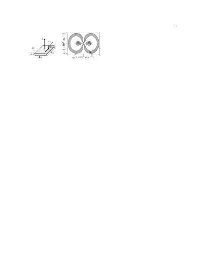
Figure 1: On left we see the thin film geometry, with magnons propagating in the $xz$-plane. On right, the regions $R_{1}$ and $R_{2}$ in quasimomentum space.

4.1 Evolution of the “Two Fluid Model”

In terms of the previous considerations we introduce the mean populations $\mathcal{N}_{1}(t)$ and $\mathcal{N}_{2}(t)$ corresponding to the relevant regions $R_{1}$ and $R_{2}$ given by

$$\mathcal{N}_{1}(t)=\frac{1}{n_{1}}\sum_{\mathbf{q}\in R_{1}}\mathcal{N}_{\mathbf{q}}(t),$$ (35)

$$\mathcal{N}_{2}(t)=\frac{1}{n_{2}}\sum_{\mathbf{q}\in R_{2}}\mathcal{N}_{\mathbf{q}}(t),$$ (36)

where $n_{1,2}={\displaystyle\sum_{\mathbf{q}\in R_{1,2}}1}$ represents the number of modes in the regions $R_{1}$ and $R_{2}$.

Proceeding correspondingly in Eq. 21, we do have that (omitting to explicitly write the time dependence on the right)

$$f_{1}{\displaystyle\frac{d}{d\bar{t}}}\mathcal{N}_{1}(\bar{t}) =-\mathrm{D}\,\mathcal{N}_{1}(\mathcal{N}_{1}-\mathcal{N}_{1}^{(0)})-f_{1}\left[\mathcal{N}_{1}-\mathcal{N}_{1}^{(0)}\right]+$$ (37)

$$+\mathrm{F}\left\{\mathcal{N}_{1}\mathcal{N}_{2}+\left(\bar{\nu}+1\right)\mathcal{N}_{2}-\bar{\nu}\mathcal{N}_{1}\right\}-$$

$$-\mathrm{M}\left\{\mathcal{N}_{1}\left(\mathcal{N}_{1}+1\right)+\mathcal{N}_{2}\left(\mathcal{N}_{2}+1\right)\right\}(\mathcal{N}_{1}\frac{\mathcal{N}_{2}^{(0)}}{\mathcal{N}_{1}^{(0)}}-\mathcal{N}_{2}),$$

and

$$f_{2}{\displaystyle\frac{d}{d\bar{t}}}\mathcal{N}_{2}(\bar{t}) =\mathrm{I}\,(1+2\mathcal{N}_{2})-$$ (38)

$$-\mathrm{D}\,\mathcal{N}_{2}(\mathcal{N}_{2}-\mathcal{N}_{2}^{(0)})-f_{2}\left[\mathcal{N}_{2}-\mathcal{N}_{2}^{(0)}\right]-$$

$$-\mathrm{F}\left\{\mathcal{N}_{1}\mathcal{N}_{2}+\left(\bar{\nu}+1\right)\mathcal{N}_{2}-\bar{\nu}\mathcal{N}_{1}\right\}+$$

$$+\mathrm{M}\left\{\mathcal{N}_{1}\left(\mathcal{N}_{1}+1\right)+\mathcal{N}_{2}\left(\mathcal{N}_{2}+1\right)\right\}(\mathcal{N}_{1}\frac{\mathcal{N}_{2}^{(0)}}{\mathcal{N}_{1}^{(0)}}-\mathcal{N}_{2}),$$

where $\bar{t}$ is the scaled time $t/\tau$, taking the relaxation time $\tau_{\mathbf{q}}$ as having a unique constant value ($\mathbf{q}$-independent), $\mathcal{N}_{1,2}^{(0)}$ are the populations in equilibrium, and $f_{1}$ and $f_{2}$ the fractions of the Brillouin zone corresponding to the two regions in the two-fluid model. Moreover, the coefficients $\mathrm{M}$ and $\mathrm{F}$ are the coupling strengths associated to magnon-magnon interaction and to Fröhlich contribution respectively, $\mathrm{D}$ is the one associated to decay with emission of photons, and $\bar{\nu}$ is an average population of the phonons; the Livshits term can be neglected. Finally, the parameter $\mathrm{I}$ is related to the rate of the rf-radiation field transferred to the spin system, whose absorption, as noticed, is reinforced by a positive feedback effect. All these coefficients are addimensional, being multiplied by the relaxation time $\tau$.

Consider now the experiment in Ref. [1]. The fractions $f_{1}$ and $f_{2}$ follows considering the size of regions $R_{1}$ and $R_{2}$, and, given the frequencies associated with these regions, the values of the mean populations in equilibrium are $\mathcal{N}_{1}^{(0)}=3\times 10^{3}$ and $\mathcal{N}_{2}^{(0)}=2\times 10^{3}$. An effective absorbed power of $10^{-2}\,\mathrm{W}$ would correspond to $\mathrm{I}\approx 10^{-3}$. On the other hand, an estimate of the $\mathcal{N}_{2}$ steady state value allows to evaluate that $\mathrm{D}\approx 10^{-11}$. On the basis of a transient time for attaining internal thermalization near equilibrium of the order of $200\,\mathrm{ns}$, it can be estimated that $\mathrm{M}\lesssim 10^{-12}$. Being $\tau$ of the order of a few microseconds (and adopting $\tau=1\,\mathrm{\mu s}$), we are left with $\mathrm{F}$ as the only open parameter.

Using the experimental data [1], varying the values of the parameters around those given above and adjusting $\mathrm{F}$, it follows the good agreement of theory and experiment shown in Fig. 2.

We proceed to analyse the several processes leading to the increase of the populations in Fig. 2, that are described in Fig. 3 in terms of the rates of increase and decay, the contributions present on the right of equations (37) and (38). Multiplying these rates by the total number of magnon modes $n\simeq 3\times 10^{14}$, we obtain the rates related to the total number of magnons in regions $R_{1}$ and $R_{2}$.

Figure 2: Evolution of the magnon population. Circles represent Demokritov’s et al. data for the low energy magnon population [1], with the pumping being switched off after $1\,\mathrm{\mu s}$. Solid lines show magnon populations of low and high energy, obtained after numerical integration of Eqs. (37) and (38) using the following parameters: $f_{1}=3\times 10^{-6}$; $f_{2}=3\times 10^{-4}$; $\mathcal{N}_{1}^{(0)}=3\times 10^{3}$; $\mathcal{N}_{2}^{(0)}=2\times 10^{3}$; $\mathrm{I}=8\times 10^{-4}$; $\mathrm{D}=4\times 10^{-11}$; $\mathrm{M}=3\times 10^{-14}$; $\mathrm{F}=2\times 10^{-6}$.

Besides the rate of pumping from the external source (designated by $\mathrm{I}$), are present the contribution arising out from Fröhlich effect, which is a pumping term for $\mathcal{N}_{1}$ and a decay one for $\mathcal{N}_{2}$, and the contribution due to magnon-magnon interaction, which redistributes the pumped energy among the modes, tending to drive the system to nonequilibrium internal thermalization (non-scattering mechanisms, i.e., decay and emission are discarded for not being of relevance: energy and momentum conservation are impaired[28]). These two effects (whose composition is referred as $\mathrm{F}+\mathrm{M}$) are responsible for internal interaction of magnons $\mathcal{N}_{1}$ and $\mathcal{N}_{2}$. Two other contributions correspond to decay, namely, a linear term of decay to the lattice ($\mathrm{L}$) and the bilinear one of decay by photon emission ($\mathrm{D}$). The sign ($+$) for pumping and ($-$) for decay is indicated in the inset.

During the time interval when the pumping is on, the source creates magnons on region $R_{2}$, while internal interactions (Fröhlich and magnon-magnon) annihilate them. These internal interactions are responsible for creating magnons in region $R_{1}$, that decay mainly through photon emission. Thus, the nonequilibrium two-fluid system has the energy pumped on region $R_{2}$, transferred to region $R_{1}$ via the composition of Fröhlich and magnon-magnon effects and while being lost through photon emission.

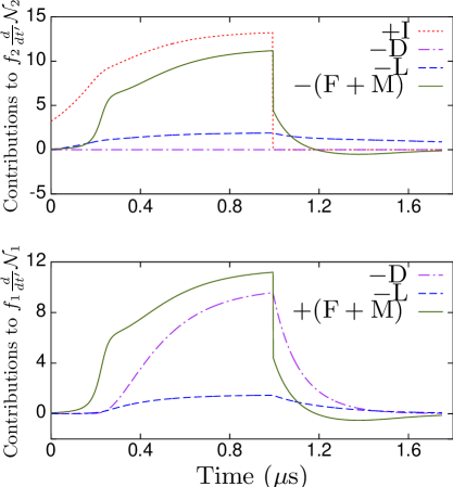
Figure 3: (Color online) Contributions (scaled) from all the distinct processes to the evolution of $\mathcal{N}_{1}$ and $\mathcal{N}_{2}$. With the same parameters used in Fig. 2, we plotted the rates of decay ($-$) and increase ($+$) of $\mathcal{N}_{2}$ (top) and $\mathcal{N}_{1}$ (bottom).

The interplay of all these processes changes as the rate of the pumping source is changed. The results reported above are for the scaled rate $\mathrm{I}=8\times 10^{-4}\,\mathrm{\mu\mbox{s}^{-1}}$.

4.2 The Steady State

Using the same parameters but considering constant application of the pumping source, the steady-state populations are obtained as a function of the source scaled rate of pumping, what is shown in Fig. 4. It can be noticed the existence of a critical pumping scaled rate (better saying, a rate threshold) after which there follows a steep increase in the population of the mode lowest in frequency, characterized by $\mathcal{N}_{1}$, corresponding to the emergence of BEC. With increasing pumping intensity a second critical rate (rate threshold) is evidenced such that for higher values of $\mathrm{I}$ is observed internal thermalization of the magnons which acquire a common quasi-temperature [cf. Eq. (34)]. This implies that the magnon-magnon interaction overcomes Fröhlich contribution and BEC is impaired.

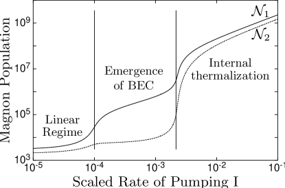
Figure 4: Steady-state magnon populations [solutions of Eqs. (37) and (38)] as a function of the scaled rate of pumping due to the source, using the same parameters as in Figure 2. It can be noticed the existence of a window for the emergence of BEC, which follows at a certain threshold of intensity. In the linear regime, at low intensity, no particular complex behaviour follows, and at high levels of intensity magnon-magnon interaction overcomes Fröhlich contribution and there follows internal thermalization.

Figure 5: Steady-state magnon populations as a function of the scaled rate of pumping when Fröhlich term is disregarded ($\mathrm{F}=0$).

Figure 6: Steady-state magnon populations as a function of the scaled rate of pumping when magnon-magnon interaction is disregarded ($\mathrm{M}=0$).

We can better appreciate the role of both types of interactions in figures 5 and 6. In Fig. 5 the Fröhlich contribution is “switched off” ($\mathrm{F}=0$), and the action of the magnon-magnon leading to internal thermalization (for $\mathrm{I}>3\times 10^{-4}$) is evidenced.

On the contrary, in Fig. 6 where the magnon-magnon interaction is “switched off” ($\mathrm{M}=0$), the emergence of NEFBEC (for $\mathrm{I}>10^{-4}$) does follow unimpeded by the magnon-magnon interaction.

Returning to Fig. 4, let us consider the interplay of the several mechanisms that lead to the formation of the steady state, when the rates of change are balanced. The rate of change associated with all the mentioned processes, in the steady state, for a range of values of the (scaled) rate of pumping from the external source, are shown in figure 7, in the upper part for $\mathcal{N}_{2}$ and in the lower part for $\mathcal{N}_{1}$, using the same notation of Fig. 3. It can be noticed the presence of three regimes in correspondence with those indicated in Fig. 4. In all cases energy is fed to the system through the “$\mathcal{N}_{2}$ magnons” pumped by the source, while Fröhlich and magnon-magnon redistribute it, creating “$\mathcal{N}_{1}$ magnons”. In the range of scaled pumping rates up to roughly $6\times 10^{-5}$, the linear regime, both $\mathcal{N}_{1}$ and $\mathcal{N}_{2}$ magnons are relaxing predominantly through the linear decay to the lattice. For greater intensities the linear decay to the lattice is not sufficient to wholly absorb the system energy in order to maintain the steady state. Thus, it is observed an increase on the $\mathcal{N}_{1}$ populations, characterizing the condensate, and in order to maintain the system stationary other relaxation mechanisms become predominant: “$\mathcal{N}_{1}$ magnons” decay through photon emission and “$\mathcal{N}_{2}$ magnons” through the $\mathrm{F}+\mathrm{M}$ term. Finally, for $\mathrm{I}\gtrsim 2\times 10^{-3}$, the non-linear photon emission decay gains relevance, the $\mathcal{N}_{2}$ populations increase, and the internal thermalization regime is attained.

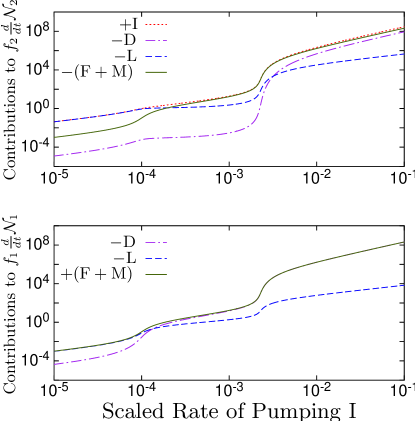
Figure 7: (Color online) Role of contributions (scaled) from all the distinct processes to the stationary state of $\mathcal{N}_{1}$ and $\mathcal{N}_{2}$. The rates for $\mathcal{N}_{2}$ (top) and $\mathcal{N}_{1}$ (bottom), with the same notation of Figure 3, are presented.

All this interplay explains, in a sense, the transition between the three regimes: In the linear regime, as the rate of energy transfer from the source increases, we have that, at low scaled rates of pumping, the populations attain values near the equilibrium ones, the usual linear relaxation to the lattice, with a characteristic relaxation time, predominates and no particular complex behavior is to be expected. As the intensity approaches a threshold value, the nonlinear contributions, associated to Fröhlich effect, magnon-magnon interactions and photon emission, begin to be relevant as the populations increase to values much greater than in equilibrium. Fröhlich effect leads to the emergence of BEC once it overcomes the tendency for internal thermalization promoted by the magnon-magnon interaction, and the decay by photon emission ensures that a steady state is attained. The second threshold in intensity value follows as magnon-magnon interaction overcomes Fröhlich effect and internal thermalization is ensured.

Moreover, considering the quantity $\Gamma_{\mathbf{q}}$ of Eqs. 26 and 27, in this two-fluid model we do have for $\Gamma_{1}$ and $\Gamma_{2}$ (mean values of $\Gamma_{\mathbf{q}}$ in regions $R_{1}$ and $R_{2}$) that

$$\Gamma_{1}(\bar{t})= \mathrm{D}\,(\mathcal{N}_{1}-\mathcal{N}_{1}^{(0)})+f_{1}-\mathrm{F}\,(\mathcal{N}_{2}-\bar{\nu})+$$ (39)

$$+\mathrm{M}\left\{\frac{\mathcal{N}_{2}^{(0)}}{\mathcal{N}_{1}^{(0)}}\left[\mathcal{N}_{1}\left(\mathcal{N}_{1}+1\right)+\mathcal{N}_{2}\left(\mathcal{N}_{2}+1\right)\right]-\left(\mathcal{N}_{1}+1\right)\mathcal{N}_{2}\right\},$$

and

$$\Gamma_{2}(\bar{t})= -2\mathrm{I}+\mathrm{D}\,(\mathcal{N}_{2}-\mathcal{N}_{2}^{(0)})+f_{2}+\mathrm{F}\,\left(\mathcal{N}_{1}+\bar{\nu}+1\right)+$$ (40)

$$\vspace{-3cm}+\mathrm{M}\left\{\mathcal{N}\left(\mathcal{N}_{1}+1\right)+\mathcal{N}_{2}\left(\mathcal{N}_{2}+1\right)-\frac{\mathcal{N}_{2}^{(0)}}{\mathcal{N}_{1}^{(0)}}\mathcal{N}_{1}\left(\mathcal{N}_{2}+1\right)\right\},$$

which have their stationary values shown in Fig. 8 as a function of the rate of pumping $\mathrm{I}$.

Figure 8: Values of $\Gamma_{1,2}$ in the steady state (cf. Eqs. 39 e 40) associated with the magnon populations (Figure 4).

According to the considerations presented in section 3, we see that $\Gamma_{\mathbf{q}}$ is the linear decay rate of the amplitudes, $\left\langle\hat{c}_{\mathbf{q}}^{\dagger}|t\right\rangle$ and $\left\langle\hat{c}_{\mathbf{q}}|t\right\rangle$. All the obtained values of $\Gamma_{1,2}$ are positive, (Fig. 8), indicating decay of these amplitudes, which corroborates the assumed neglect of their contribution to the populations’ evolution. Although the amplitudes decay, we point that in the source intensity interval associated with the condensate, $10^{-4}\lesssim\mathrm{I}\lesssim 2\times 10^{-3}$, $\Gamma_{1}$ is considerably smaller than $\Gamma_{2}$, and the condensate would allow long mean-life to the coherent states corresponding to the lowest frequency modes, which can be excited to compose solitary waves, as it has been shown in the case of other boson systems displaying NEFBEC [14, 18, 20].

The decay of the populations after the switching off of the pumping source follows in accord with the one observed in the experiment of Ref. [58]. It consists of three regimes: a near exponential one at the initial delay times (scaled time in the interval $1$ to $\sim 1.7$ in Fig. 2), with scaled decay time of $0.23$, and another with a scaled decay time of $1.02$ when approaching final equilibrium (after scaled time $\sim 2.5$ in Fig. 2) and an intermediate one in between (roughly the interval from $1.7$ to $2.5$ in scaled time in Fig. 2) as shown in next subsection.

4.3 Decay of the Condensate

In Ref. [58] is reported by Demidov et al. an analysis of the decay, towards final equilibrium, of the NEBEC in YIG, after the external rf-pumping source has been switched off. There are some differences in the experimental protocol with respect to the one used in Ref. [1], but we analyse the decay in the conditions of the latter, to study the dependence (as done in the experiment of Ref. [58]) with the source power.

Using Eqs. (37) and (38) in Subsection 4.1, the one that leads to the results of Fig. 2, varying the values of the rate of pumping $\mathrm{I}$ we obtain the set of curves for the evolution of the population in the condensate shown in Fig. 9.

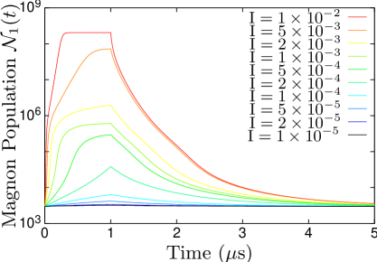
Figure 9: (Color online) Time evolution of the condensate ($\mathcal{N}_{1}$) for different values of the rate of pumping $\mathrm{I}$.

It may be noticed the interesting result that these curves can be approximately well adjusted by the law

$$\mathcal{N}_{1}(t)-\mathcal{N}_{1}^{(0)}=A\,\exp\left(-\nicefrac{{t}}{{\tau_{\mathrm{A}}}}\right)+B\,\exp\left(-\nicefrac{{t}}{{\tau}}\right),$$ (41)

The fitting values of the two coefficients, $A$ and $B$, and the characteristic decay time $\tau_{\mathrm{A}}$ are indicated in Table 1; $\tau$ is the relaxation time to the lattice.

Table 1: Coefficients $A$, $B$ and $\tau_{\mathrm{A}}$ obtained from the fitting of Eq. 41 to the numerical data presented in Fig. 9 (it has been taken $\tau=1\,\mathrm{\mu s}$).

$\mathrm{I}$	$\tau_{\mathrm{A}}\,\mathrm{(\mu s)}$	$A$	$B$
$5\times 10^{-5}$	$0,47670$	$140,10$	$1064,48$
$6\times 10^{-5}$	$0,46853$	$217,96$	$1316,59$
$8\times 10^{-5}$	$0,45151$	$458,56$	$1869,11$
$10\times 10^{-5}$	$0,4326$	$863,2$	$2496,7$
$13\times 10^{-5}$	$0,3990$	$2006,9$	$3618,7$
$16\times 10^{-5}$	$0,3568$	$4460$	$5048$
$20\times 10^{-5}$	$0,2849$	$1,3603\times 10^{4}$	$7786$
$25\times 10^{-5}$	$0,2131$	$5,890\times 10^{4}$	$1,278\times 10^{4}$
$32\times 10^{-5}$	$0,21706$	$1,5904\times 10^{5}$	$1,523\times 10^{4}$
$40\times 10^{-5}$	$0,22634$	$2,3599\times 10^{5}$	$1,524\times 10^{4}$
$50\times 10^{-5}$	$0,23113$	$3,0488\times 10^{5}$	$1,517\times 10^{4}$
$63\times 10^{-5}$	$0,23310$	$3,7937\times 10^{5}$	$1,544\times 10^{4}$
$79\times 10^{-5}$	$0,23263$	$4,6423\times 10^{5}$	$1,636\times 10^{4}$
$100\times 10^{-5}$	$0,22948$	$5,765\times 10^{5}$	$1,852\times 10^{4}$
$126\times 10^{-5}$	$0,22314$	$7,315\times 10^{5}$	$2,29\times 10^{4}$
$158\times 10^{-5}$	$0,2124$	$9,765\times 10^{5}$	$3,17\times 10^{4}$

Clearly, we can say that there exist three reasonably well defined regimes: one immediately after the switching-off of the source, other at longer decay times when the population is approaching the final value at equilibrium, and, of course, an intermediate one.

In Fig. 10 we indicate the decay time $\tau_{\mathrm{A}}$ as a function of the scaled rate of pumping $\mathrm{I}$.

Figure 10: Decay time $\tau_{A}$ of the condensate as a function of the pumping parameter $\mathrm{I}$.

It can be noticed a qualitative agreement with the experimental data of Demidov et al. in figure 3 of reference [58], namely, a sigmoid-like curve up to $\mathrm{I}\sim 1\times 10^{-3}$, except for the central dip in an intermediate region where no experimental data are reported. We proceed to study in detail the different relaxation processes that produce these results.

We analyse (using the same notation for rates of the previous section) the relaxation processes involved: (i) the linear relaxation to the lattice ($\mathrm{L}$-process); (ii) the radiative decay ($\mathrm{D}$-process); (iii) the conjugated effect of magnon-magnon interaction and Fröhlich effect [$(\mathrm{F}+\mathrm{M})$-process].

At small $\mathrm{I}$, as stated before, the $\mathrm{L}$-process dominates the decay. But, for intensities such that Eq. 41 applies to the populations decay (see figure 9), it can be noticed the increasing relevance of the $\mathrm{F}+\mathrm{M}$-process, as can be seen in Fig. 11a (Regime I). While the pumping source is acting, Fröhlich and magnon-magnon terms transfer the energy from the fed magnons ($\mathcal{N}_{2}$) to the ones in the condensate ($\mathcal{N}_{1}$), but after turning off the source the flux of energy is inverted, and $\mathrm{F}+\mathrm{M}$-processes become another mechanism of relaxation of the condensate, thus reducing $\tau_{A}$. Progressive amplification of the pumping power enlarge this effect, as shown in Fig. 10. A minimum $\tau_{A}$ value is achieved for $\mathrm{I}\simeq 2,5\times 10^{-4}$ (Fig. 11b) and then, for higher $\mathrm{I}$, the $\mathrm{F}+\mathrm{M}$-process, dominant relaxation process until that intensity, diminish, and the $\mathrm{D}$-process begins to increase. Then, the decay time $\tau_{A}$ increases until the $\mathrm{D}$-process dominates the relaxation (Fig. 11c) and, after this point, where is initiated the Regime III, $\tau_{A}$ starts to decrease again. For values of $\mathrm{I}$ higher than $2\times 10^{-3}$, the relaxation in the condensate does not follow Eq. 41.

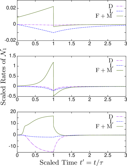
Figure 11: (Color online) Scaled rates of creation and annihilation of magnons in $R_{1}$ region for different scaled pumping rates. On the upper figure, with $\mathrm{I}=10^{-4}$, in Regime I, the linear relaxation is predominant, but the $\mathrm{F}+\mathrm{M}$-process gains relevance. On the central figure, in Regime II, with $\mathrm{I}=2,5\times 10^{-4}$, and the $\mathrm{F}+\mathrm{M}$-process is the principal relaxation mechanism. Finally, on the lower figure, we have in Regime III, with $\mathrm{I}=10^{-3}$, where the $\mathrm{D}$-process dominates the relaxation.

Thus we conclude that, depending on the populations $\mathcal{N}_{1}$ and $\mathcal{N}_{2}$, immediately after turning off the pumping source, the three distinct contributions indicated rule the condensate relaxation. Briefly, it can be stated that increasing the pumping source intensity before turning it off changes the dominant relaxation process in the following order:

$$\mathrm{L}\to\mathrm{F}+\mathrm{M}\to\mathrm{D},$$

explaining in this way the unexpected behaviour of $\mathcal{N}_{1}$ while returning to equilibrium.

5 Concluding Remarks

In summary, as experimentally evidenced by Demokritov et al. the spin system in magnetic thin films under excitation by rf-radiation, display a phenomenon of the type of a Bose-Einstein condensation of the hot magnons [1]. The theoretical analysis performed here, in terms of a nonequilibrium statistical thermo-mechanics, shows that, in fact, this BEC of magnons follows in the way expected for many-boson systems embedded in a thermal bath as firstly demonstrated by H. Fröhlich [11, 12], and we may cite him who, in his original work (the case of biopolymers), stated that

“… under appropriate conditions a phenomenon quite similar to Bose condensation may occur in substances which possess longitudinal electric modes. If energy is fed into these modes and thence transferred to other degrees of freedom of the substance then a stationary state will be reached in which the energy content of the electric modes is larger than in thermal equilibrium. This excess energy is found to be channelled into a single mode – exactly as in Bose condensation – provided the energy supply exceeds a critical value. Under these circumstances a random supply of energy is thus not completely thermalized but partly used in maintaining a coherent electric wave in the substance.”

Moreover, that long-lived solitons (in the form of a statistically averaged macroscopic wave function of coherent states) propagate in the condensate, Finally, it can be noticed that the extended analysis of the nonequilibrium thermodynamics of the phenomenon described in the Refs. [14] is formally identical to the one that can be applied to the magnons embedded in the lattice we have considered here, which is to be extensively described in a forthcoming article.

Appendix A The Hamiltonian of the Magnon System

To introduce the magnon creation (annihilation) operators, we use the Holstein-Primakoff transformation [28, 29, 30]: at first, spin operators are expressed in terms of local bosonic creation (annihilation) operators, $\hat{a}_{j}^{\dagger}$ ($\hat{a}_{j}$),

$$\hat{S}_{j}^{x}=\frac{\sqrt{2S}}{2}\left[\left(1-\frac{\hat{a}_{j}^{\dagger}\hat{a}_{j}}{2S}\right)^{\nicefrac{{1}}{{2}}}\hat{a}_{j}+\hat{a}_{j}^{\dagger}\left(1-\frac{\hat{a}_{j}^{\dagger}\hat{a}_{j}}{2S}\right)^{\nicefrac{{1}}{{2}}}\right],$$

$$\hat{S}_{j}^{y}=\frac{\sqrt{2S}}{2i}\left[\left(1-\frac{\hat{a}_{j}^{\dagger}\hat{a}_{j}}{2S}\right)^{\nicefrac{{1}}{{2}}}\hat{a}_{j}-\hat{a}_{j}^{\dagger}\left(1-\frac{\hat{a}_{j}^{\dagger}\hat{a}_{j}}{2S}\right)^{\nicefrac{{1}}{{2}}}\right],$$

$$\hat{S}_{j}^{z}=S-\hat{a}_{j}^{\dagger}\hat{a}_{j}.$$ (42)

We consider a crystaline material with $N_{\mathrm{c}}$ unit cells, with the ionic position $\mathbf{R}_{i}$ given by the position $\mathbf{r}_{n}$ of the unit cell $n$ and the internal relative position $\mathbf{d}_{\mu}$,

$$\mathbf{R}_{i}=\mathbf{r}_{n}+\mathbf{d}_{\mu},$$ (43)

with $\mu$ designating the internal ions ($\mu=1,2,\dots$ until the number of magnetic ions included in the unit cell), and it is introduced the Fourier expansion,

$$\hat{a}_{j}=\sum_{\mathbf{q},\mu}\frac{\mbox{e}^{i(\mathbf{q}\cdot\mathbf{R}_{j})}}{\sqrt{N_{\mathrm{c}}}}\hat{a}_{\mathbf{q},\mu},$$ (44)

being $\mathbf{q}$ the wave vector running over the first Brillouin zone. Collecting only the quadratic terms of $\hat{\mathscr{H}}_{\mathrm{exc}}+\hat{\mathscr{H}}_{\mathrm{dip}}+\hat{\mathscr{H}}_{\mathrm{Z}}$ [Eqs. (2), (3) and (4)] in what we call $\hat{\mathscr{H}}_{\mathrm{S}}^{(2)}$, one obtains

$$\hat{\mathscr{H}}_{\mathrm{S}}^{(2)} =\sum_{\mathbf{q},\mu,\mu^{\prime}}\Biggl{\{}\mathrm{A}^{\prime}_{\mu\mu^{\prime}}(\mathbf{q})\,\hat{a}_{\mathbf{q},\mu}^{\dagger}\hat{a}_{\mathbf{q},\mu^{\prime}}+$$ (45)

$$+\frac{\mathrm{B}_{\mu\mu^{\prime}}^{\prime*}(\mathbf{q})}{2}\hat{a}_{\mathbf{q},\mu}^{\dagger}\hat{a}_{-\mathbf{q},\mu^{\prime}}^{\dagger}+\frac{\mathrm{B}^{\prime}_{\mu\mu^{\prime}}(\mathbf{q})}{2}\hat{a}_{\mathbf{q},\mu}\hat{a}_{-\mathbf{q},\mu^{\prime}}\Biggr{\}},$$

with

$$\mathrm{A}^{\prime}_{\mu\mu^{\prime}}(\mathbf{q}) =\sum_{n,n^{\prime}}\left\{\mathrm{A}_{1}(\mathbf{r}_{nn^{\prime}}+\mathbf{d}_{\mu\mu^{\prime}})\mbox{e}^{i\left[\mathbf{q}\cdot(\mathbf{r}_{nn^{\prime}}+\mathbf{d}_{\mu\mu^{\prime}})\right]}+\right.$$ (46)

$$\qquad\left.+\mathrm{A}_{2}(\mathbf{r}_{nn^{\prime}}+\mathbf{d}_{\mu\mu^{\prime}})\right\},$$

$$\mathrm{B}^{\prime}_{\mu\mu^{\prime}}(\mathbf{q})=\sum_{n,n^{\prime}}\mathrm{B}(\mathbf{r}_{nn^{\prime}}+\mathbf{d}_{\mu\mu^{\prime}})\mbox{e}^{i\left[\mathbf{q}\cdot(\mathbf{r}_{nn^{\prime}}+\mathbf{d}_{\mu\mu^{\prime}})\right]},$$ (47)

where $\mathbf{r}_{nn^{\prime}}=\mathbf{r}_{n^{\prime}}-\mathbf{r}_{n}$ and with $(n,\mu)\neq(n^{\prime},\mu^{\prime})$, and

$$\mathrm{A}_{1}(\mathbf{R}_{ij})=-2SJ(R_{ij})-\frac{(g\mu_{\mathrm{B}})^{2}S}{2R_{ij}^{5}}[2R_{ij}^{2}-3(R_{ij}^{z})^{2}],$$ (48)

$$\mathrm{A}_{2}(\mathbf{R}_{ij})=2SJ(R_{ij})+\frac{g\mu_{\mathrm{B}}\mathrm{H}_{0}}{N}-\frac{(g\mu_{\mathrm{B}})^{2}S}{R_{ij}^{5}}[R_{ij}^{2}-3(R_{ij}^{z})^{2}],$$ (49)

$$\mathrm{B}(\mathbf{R}_{ij})=-\frac{3(g\mu_{\mathrm{B}})^{2}S}{2}\frac{(R_{ij}^{-})^{2}}{R_{ij}^{5}}.$$ (50)

The diagonalization of $\hat{\mathscr{H}}_{\mathrm{S}}^{(2)}$ of Eq. 45 is done through the introduction of the magnon creation and annihilation operators $\hat{c}_{\mathbf{q},\gamma}^{\dagger}$ and $\hat{c}_{\mathbf{q},\gamma}$, as linear combinations of $\hat{a}_{\mathbf{q},\mu}^{\dagger}$ and $\hat{a}_{\mathbf{q},\mu}$ in such a way that [28, 65, 66]

$$\hat{\mathscr{H}}_{\mathrm{S}}^{(2)}=\sum_{\mathbf{q},\gamma}\hbar\omega_{\mathbf{q},\gamma}\hat{c}_{\mathbf{q},\gamma}^{\dagger}\hat{c}_{\mathbf{q},\gamma}.$$ (51)

The resulting magnons, with energy $\hbar\omega_{\mathbf{q},\gamma}$ and group velocity $\nabla_{\mathbf{q}}\omega_{\mathbf{q},\gamma}$, are grouped in branches indicated by $\gamma$, in the case of more than one magnetic ion per unitary cell (see Refs. [65, 66] for the YIG). In the experiments with thin films of YIG analyzed here, only low frequency magnons are excited ($\lesssim 10\,\mathrm{GHz}$), justifying the omission of all the branches but the acoustic one. In this sense, only one effective spin per unit cell is considered, $\mu$ and $\gamma$ are omitted and we write for $\hat{\mathscr{H}}_{\mathrm{S}}^{(2)}$ of Eq. (51)

$$\hat{\mathscr{H}}_{\mathrm{S}}^{(2)}\simeq\sum_{\mathbf{q}}\hbar\omega_{\mathbf{q}}\hat{c}_{\mathbf{q}}^{\dagger}\hat{c}_{\mathbf{q}}.$$ (52)

In this situation of taking into account only the acoustic magnons, Eq. (52) follows from Eq. (45), when in the latter we take one effective spin per unit cell, after using the so-called Bogoliubov transformation, [28, 29],

$$a_{\mathbf{q}} = u_{\mathbf{q}}c_{\mathbf{q}}+v_{\mathbf{q}}^{*}c_{-\mathbf{q}}^{\dagger},$$

$$a_{-\mathbf{q}}^{\dagger} = u_{-\mathbf{q}}^{*}c_{-\mathbf{q}}^{\dagger}+v_{-\mathbf{q}}c_{\mathbf{q}},$$ (53)

with $u_{\mathbf{q}}$ and $v_{\mathbf{q}}$ functions of $\mathbf{q}$. It can be shown that

$$u_{\mathbf{q}}=\sqrt{\frac{\mathrm{A}^{\prime}(\mathbf{q})+\hbar\omega_{\mathbf{q}}}{2\hbar\omega_{\mathbf{q}}}},\quad v_{\mathbf{q}}=\frac{\mathrm{B}^{\prime}(\mathbf{q})}{\left|\mathrm{B}^{\prime}(\mathbf{q})\right|}\sqrt{\frac{\mathrm{A}^{\prime}(\mathbf{q})-\hbar\omega_{\mathbf{q}}}{2\hbar\omega_{\mathbf{q}}}},$$ (54)

and the (acoustic) magnon dispersion relation is given by

$$\hbar\omega_{\mathbf{q}}=\sqrt{\left[\mathrm{A}^{\prime}(\mathbf{q})\right]^{2}-\left|\mathrm{B}^{\prime}(\mathbf{q})\right|^{2}},$$ (55)

and Refs. [4, 67] presents recent studies on this dispersion relation in cases of thin films of YIG.

The Holstein-Primakoff and Bogoliubov transformations are then applied to the non-quadratic terms of $\hat{\mathscr{H}}_{\mathrm{exc}}+\hat{\mathscr{H}}_{\mathrm{dip}}+\hat{\mathscr{H}}_{\mathrm{Z}}$, and the magnon-magnon interaction term is then obtained. Retaining only the fourth order scattering terms, the magnon-magnon interaction which contributes to the Hamiltonian is given by

$$\hat{\mathscr{H}}_{\mathrm{MM}}=\sum_{\mathbf{q},\mathbf{q}_{1},\mathbf{q}_{2}}\mathcal{V}_{\mathbf{q},\mathbf{q}_{1},\mathbf{q}_{2}}\hat{c}_{\mathbf{q}}^{\dagger}\hat{c}_{\mathbf{q}_{1}}^{\dagger}\hat{c}_{\mathbf{q}_{2}}\hat{c}_{\mathbf{q}+\mathbf{q}_{1}-\mathbf{q}_{2}}.$$

Phonon and photon creation and annihilation operators are introduced in similar ways. The Hamiltonian of the free phonons is

$$\hat{\mathscr{H}}_{\mathrm{L}}=\sum_{\mathbf{k}}\hbar\Omega_{\mathbf{k}}\left(\hat{b}_{\mathbf{k}}^{\dagger}\hat{b}_{\mathbf{k}}+\frac{1}{2}\right),$$ (56)

with $\Omega_{\mathbf{k}}$ being their dispersion relation (we recall that only acoustic phonons were considered; polarization is implicit). The phonon creation and annihilation operators, $\hat{b}_{\mathbf{k}}^{\dagger}$ and $\hat{b}_{\mathbf{k}}$, are related to the displacement of the effective magnetic ion around the equilibrium position $\mathbf{r}_{n}$, which is

$$\mathbf{x}_{n}=\left(\frac{\hbar}{2N_{\mathrm{c}}}\right)^{\frac{1}{2}}\sum_{\mathbf{k}}\frac{\mathbf{e}(\mathbf{k})}{\sqrt{\Omega_{\mathbf{k}}}}\left(\hat{b}_{\mathbf{k}}\mbox{e}^{i\mathbf{k}\cdot\mathbf{r}_{n}}+\hat{b}_{\mathbf{k}}^{\dagger}\mbox{e}^{-i\mathbf{k}\cdot\mathbf{r}_{n}}\right),$$ (57)

and $\mathbf{e}(\mathbf{k})$ is the polarization versor (cf. Ref. [29]). Using Eq. 57 in Eq. 6, we obtain the for magnon-phonon interaction

$$\hat{\mathscr{H}}_{\mathrm{SL}} ={\displaystyle\sum_{\mathbf{q},\mathbf{k}\neq 0}}(\hat{b}_{\mathbf{k}}+\hat{b}_{-\mathbf{k}}^{\dagger})\Big{\{}\mathcal{F}_{\mathbf{q},\mathbf{k}}\hat{c}_{\mathbf{q}}^{\dagger}\hat{c}_{\mathbf{q}-\mathbf{k}}+\mathcal{L}_{\mathbf{q},\mathbf{k}}\hat{c}_{\mathbf{q}}^{\dagger}\hat{c}_{\mathbf{k}-\mathbf{q}}^{\dagger}+$$ (58)

$$\qquad\qquad\qquad\qquad+\mathcal{L}_{\mathbf{q},-\mathbf{k}}^{*}\hat{c}_{\mathbf{q}}\hat{c}_{-\mathbf{k}-\mathbf{q}}\Big{\}}+$$

$$+{\displaystyle\sum_{\mathbf{q},\mathbf{k}\neq 0}}\Big{\{}\mathcal{R}_{\mathbf{q},\mathbf{k}}\hat{b}_{\mathbf{k}}^{\dagger}\hat{b}_{\mathbf{k}-\mathbf{q}}+\mathcal{R}_{\mathbf{q},\mathbf{k}}^{+}\hat{b}_{\mathbf{k}}^{\dagger}\hat{b}_{\mathbf{q}-\mathbf{k}}^{\dagger}+$$

$$\qquad+\mathcal{R}_{-\mathbf{q},-\mathbf{k}}^{+*}\hat{b}_{-\mathbf{k}}\hat{b}_{\mathbf{k}-\mathbf{q}}\Big{\}}(\hat{c}_{\mathbf{q}}+\hat{c}_{-\mathbf{q}}^{\dagger}),$$

where $\mathcal{F}_{\mathbf{q},\mathbf{k}}$, $\mathcal{L}_{\mathbf{q},\mathbf{k}}$ and $\mathcal{R}_{\mathbf{q},\mathbf{k}}^{(\pm)}$ are the resulting coefficients (representing the interaction coupling intensities). We write for the field generated by photons of the electromagnetic fields (from the source and black-body radiation) [68]

$$\mathbf{H}(\mathbf{r})=\sum_{\alpha,\mathbf{p}}(\mathbf{H}_{\alpha,\mathbf{p}}(\mathbf{r})\,\hat{d}_{\alpha,\mathbf{p}}+\mathbf{H}_{\alpha,\mathbf{p}}^{*}(\mathbf{r})\,\hat{d}_{\alpha,\mathbf{p}}^{\dagger}),$$ (59)

where $\hat{d}_{\alpha,\mathbf{q}}$ ($\hat{d}_{\alpha,\mathbf{q}}^{\dagger}$) are the photon creation (annihilation) operators,

$$\mathbf{H}_{\alpha,\mathbf{p}}(\mathbf{r})=i\mathbf{p}\times\mathbf{A}_{\alpha,\mathbf{p}}(\mathbf{r}),\qquad\mathbf{A}_{\alpha,\mathbf{p}}(\mathbf{r})=\sqrt{\frac{2\pi}{\zeta_{\mathbf{p}}}}\mbox{e}^{i\mathbf{p}\cdot\mathbf{r}}\mathbf{e}^{(\alpha)},$$ (60)

$\zeta_{\mathbf{p}}$ is the photon angular frequency, $\mathbf{p}$ its linear moment and $\mathbf{e}^{(\alpha)}$ the polarization vector (the different polarizations are indexed by $\alpha$).

After some algebra, we obtain for the magnon-photon interaction of Eq. 5 the expression

$$\hat{\mathscr{H}}_{\mathrm{SR}} =\sum_{\alpha,\mathbf{p}}(\hat{d}_{\alpha,\mathbf{p}}+\hat{d}_{\alpha,-\mathbf{p}}^{\dagger})\left(\mathcal{S}_{\alpha,\mathbf{p}}^{\perp*}\hat{c}_{\mathbf{p}}^{\dagger}+\mathcal{S}_{\alpha,-\mathbf{p}}^{\perp}\hat{c}_{-\mathbf{p}}\right)+$$ (61)

$$+\sum_{\alpha,\mathbf{p},\mathbf{q}}(\hat{d}_{\alpha,\mathbf{p}}+\hat{d}_{\alpha,-\mathbf{p}}^{\dagger})\Big{\{}\mathcal{S}_{\alpha,\mathbf{q},\mathbf{p}}^{\parallel\mathrm{a}}\hat{c}_{\mathbf{q}}^{\dagger}\hat{c}_{\mathbf{q}-\mathbf{p}}+v_{\mathbf{q}}v_{\mathbf{q}-\mathbf{p}}^{*}+$$

$$\qquad+\mathcal{S}_{\alpha,\mathbf{q},\mathbf{p}}^{\parallel\mathrm{b}}\hat{c}_{\mathbf{q}}^{\dagger}\hat{c}_{\mathbf{p}-\mathbf{q}}^{\dagger}+\mathcal{S}_{\alpha,-\mathbf{q},-\mathbf{p}}^{\parallel\mathrm{b}*}\hat{c}_{-\mathbf{q}}\hat{c}_{\mathbf{q}-\mathbf{p}}\Big{\}},$$

where $\mathcal{S}_{\alpha,\mathbf{p}}^{\perp*}$, $\mathcal{S}_{\alpha,\mathbf{q},\mathbf{p}}^{\parallel\mathrm{a}}$ and $\mathcal{S}_{\alpha,\mathbf{q},\mathbf{p}}^{\parallel\mathrm{b}}$ are intensity coupling coefficients. Considering that the external pumping source and black-body radiation are the origins of the electromagnetic fields, we can distinguish respectively their operators as $\hat{d}_{\alpha,\mathbf{q}}^{\mathrm{S}}$ and $\hat{d}_{\alpha,\mathbf{q}}^{\,\mathrm{T}}$, and the energy of the black-body radiation is

$$\hat{\mathscr{H}}_{\mathrm{R}}=\sum_{\alpha,\mathbf{p}}\hbar\zeta_{\mathbf{p}}\left(\hat{d}_{\alpha,\mathbf{q}}^{\,\mathrm{T}\dagger}\hat{d}_{\alpha,\mathbf{q}}^{\,\mathrm{T}}+\frac{1}{2}\right).$$ (62)

The complete Hamiltonian is then written, in second quantization form, as

$$\hat{\mathscr{H}}= \sum_{\mathbf{q}}\hbar\omega_{\mathbf{q}}\hat{c}_{\mathbf{q}}^{\dagger}\hat{c}_{\mathbf{q}}+\sum_{\mathbf{k}}\hbar\Omega_{\mathbf{k}}\hat{b}_{\mathbf{k}}^{\dagger}\hat{b}_{\mathbf{k}}+\sum_{\alpha,\mathbf{p}}\hbar\zeta_{\mathbf{p}}\hat{d}_{\alpha,\mathbf{q}}^{\dagger}\hat{d}_{\alpha,\mathbf{q}}+$$

$$+\sum_{\mathbf{q},\mathbf{q}_{1},\mathbf{q}_{2}}\mathcal{V}_{\mathbf{q},\mathbf{q}_{1},\mathbf{q}_{2}}\hat{c}_{\mathbf{q}}^{\dagger}\hat{c}_{\mathbf{q}_{1}}^{\dagger}\hat{c}_{\mathbf{q}_{2}}\hat{c}_{\mathbf{q}+\mathbf{q}_{1}-\mathbf{q}_{2}}+$$

$$+{\displaystyle\sum_{\mathbf{q},\mathbf{k}\neq 0}}(\hat{b}_{\mathbf{k}}+\hat{b}_{-\mathbf{k}}^{\dagger})\left\{\mathcal{F}_{\mathbf{q},\mathbf{k}}\hat{c}_{\mathbf{q}}^{\dagger}\hat{c}_{\mathbf{q}-\mathbf{k}}+\mathcal{L}_{\mathbf{q},\mathbf{k}}\hat{c}_{\mathbf{q}}^{\dagger}\hat{c}_{\mathbf{k}-\mathbf{q}}^{\dagger}+\mathcal{L}_{\mathbf{q},-\mathbf{k}}^{*}\hat{c}_{\mathbf{q}}\hat{c}_{-\mathbf{k}-\mathbf{q}}\right\}+$$

$$+{\displaystyle\sum_{\mathbf{q},\mathbf{k}\neq 0}}\left\{\mathcal{R}_{\mathbf{q},\mathbf{k}}\hat{b}_{\mathbf{k}}^{\dagger}\hat{b}_{\mathbf{k}-\mathbf{q}}+\mathcal{R}_{\mathbf{q},\mathbf{k}}^{+}\hat{b}_{\mathbf{k}}^{\dagger}\hat{b}_{\mathbf{q}-\mathbf{k}}^{\dagger}+\mathcal{R}_{-\mathbf{q},-\mathbf{k}}^{+*}\hat{b}_{-\mathbf{k}}\hat{b}_{\mathbf{k}-\mathbf{q}}\right\}(\hat{c}_{\mathbf{q}}+\hat{c}_{-\mathbf{q}}^{\dagger})+$$

$$+\sum_{\alpha,\mathbf{p}}(\hat{d}_{\alpha,\mathbf{p}}+\hat{d}_{\alpha,-\mathbf{p}}^{\dagger})\left(\mathcal{S}_{\alpha,\mathbf{p}}^{\perp*}\hat{c}_{\mathbf{p}}^{\dagger}+\mathcal{S}_{\alpha,-\mathbf{p}}^{\perp}\hat{c}_{-\mathbf{p}}\right)+$$

$$+\sum_{\alpha,\mathbf{p},\mathbf{q}}(\hat{d}_{\alpha,\mathbf{p}}+\hat{d}_{\alpha,-\mathbf{p}}^{\dagger})\left\{\mathcal{S}_{\alpha,\mathbf{q},\mathbf{p}}^{\parallel\mathrm{a}}\hat{c}_{\mathbf{q}}^{\dagger}\hat{c}_{\mathbf{q}-\mathbf{p}}+\mathcal{S}_{\alpha,\mathbf{q},\mathbf{p}}^{\parallel\mathrm{b}}\hat{c}_{\mathbf{q}}^{\dagger}\hat{c}_{\mathbf{p}-\mathbf{q}}^{\dagger}+\mathcal{S}_{\alpha,\mathbf{q},-\mathbf{p}}^{\parallel\mathrm{b}*}\hat{c}_{-\mathbf{q}}\hat{c}_{\mathbf{q}-\mathbf{p}}\right\}.$$

Appendix B The Nonequilibrium Statistical Operator

The nonequilibrium statistical operator is given by [31, 32, 33, 34, 35, 36]

$$\hat{\mathscr{R}}_{\varepsilon}(t)=\hat{\varrho}_{\varepsilon}(t)\times\hat{\varrho}_{\mathrm{B}},$$ (64)

where

$$\hat{\varrho}_{\varepsilon}(t)=\exp\left\{\ln\hat{\bar{\rho}}(t,0)-\int_{t_{0}}^{t}dt^{\prime}\mbox{e}^{\varepsilon\left(t^{\prime}-t\right)}\frac{d}{dt^{\prime}}\ln\hat{\bar{\rho}}(t^{\prime},t^{\prime}-t)\right\}$$ (65)

is the nonequilibrium statistical operator of the magnon system, with the auxiliary statistical operator $\hat{\bar{\rho}}$ (also called “instantaneous quasi-equilibrium operator”), depending (superoperator) on the basic microvariables of set 14, given by

$$\hat{\bar{\rho}}(t,0)=\; \exp\Biggl{\{}-\Phi(t)-{\displaystyle\sum_{\mathbf{q}}}\left[F_{\mathbf{q}}(t)\hat{c}_{\mathbf{q}}^{\dagger}\hat{c}_{\mathbf{q}}+\right.$$ (66)

$$\qquad+\phi_{\mathbf{q}}(t)\hat{c}_{\mathbf{q}}+\phi_{\mathbf{q}}^{*}(t)\hat{c}_{\mathbf{q}}^{\dagger}+$$

$$\left.\qquad+\varphi_{\mathbf{q}}(t)\hat{c}_{\mathbf{q}}\hat{c}_{-\mathbf{q}}+\varphi_{\mathbf{q}}^{*}(t)\hat{c}_{\mathbf{q}}^{\dagger}\hat{c}_{-\mathbf{q}}^{\dagger}\right]\Biggr{\}}$$

after recalling that we haze neglected local inhomogeneities. In $\bar{\rho}(t^{\prime},t^{\prime\prime})$the first term in the argument, $t^{\prime}$, refers to the evolution in time of the nonequilibrium thermodynamic state of the system (i.e., of the nonequilibrium thermodynamic variables $F_{\mathbf{q}}(t)$, $\phi_{\mathbf{q}}(t)$ and $\varphi_{\mathbf{q}}(t)$), and the second, $t^{\prime\prime}$, to the evolution of the microdynamical variables $\hat{\mathcal{N}}_{\mathbf{q}}$, $\hat{c}_{\mathbf{q}}$ and $\hat{\sigma}_{\mathbf{q}}$ in Heisenberg representation. $\varepsilon$ is a positive infinitesimal that goes to $+0$ after calculation of average values has been performed. Moreover, $\Phi(t)$ ensures the normalization of the probability distributions, and plays the role of the logarithm of a nonequilibrium partition function: $\Phi(t)=\ln\bar{Z}(t)$. It is verified that

$$\mathcal{N}_{\mathbf{q}}(t)=\frac{\delta\ln\bar{Z}}{\delta F_{\mathbf{q}}(t)},$$ (67)

and similarly for the other quantities, in complete analogy with the situation in equilibrium, meaning that $F_{\mathbf{q}}(t)$ and the others in set (15) are the nonequilibrium thermodynamic variables said conjugated to the basic variables in set (16). Furthermore, it is verified that

$$\hat{\varrho}_{\varepsilon}(t)=\hat{\bar{\rho}}(t,0)+\hat{\varrho}^{\prime}_{\varepsilon}(t),$$ (68)

where $\hat{\varrho}^{\prime}_{\varepsilon}(t)$ incorporates irreversibility and historicity. In Eq. 64

$$\hat{\varrho}_{\mathrm{B}}=Z_{\mathrm{B}}^{-1}(T_{0})\exp\left\{\frac{\hat{\mathscr{H}}_{\mathrm{L}}+\hat{\mathscr{H}}_{\mathrm{R}}}{k_{\mathrm{B}}T_{0}}\right\}$$ (69)

is the canonical distribution function of the phonons and photons in equilibrium at temperature $T_{0}$.

Appendix C The Evolution Equations for the Basic Variables

The macrovariable $Q_{j}$ [a generic expression for those of the set indicated in Eq. (16)], related to the microdynamical one $\hat{P_{j}}$ [of the set in Eq. (14)], has its evolution given by the Heisenberg equation of motion weighted with the nonequilibrium statistical operator $\hat{\mathscr{R}}_{\varepsilon}(t)$, namely

$$\frac{\partial}{\partial t}Q_{j}(t)=\frac{1}{i\hbar}\mbox{Tr}\left\{\left[\hat{P}_{j},\hat{\mathscr{H}}\right]\,\hat{\mathscr{R}}_{\varepsilon}(t)\right\},$$ (70)

which, considering Eq. (64) and that, according to 68, $\hat{\varrho}^{\prime}_{\varepsilon}(t)=\hat{\varrho}_{\varepsilon}(t)-\hat{\bar{\varrho}}(t,0)$, can be rewritten as

$$\frac{\partial}{\partial t}Q_{j}(t)=J_{Q_{j}}^{(0)}(t)+J_{Q_{j}}^{(1)}(t)+\mathcal{J}_{Q_{j}}(t),$$ (71)

with

$$J_{Q_{j}}^{(0)}(t)\equiv\frac{1}{i\hbar}\mbox{Tr}\left\{\left[\hat{P}_{j},\hat{\mathscr{H}}^{0}\right]\,\hat{\bar{\varrho}}(t,0)\times\varrho_{\mathrm{B}}\right\},$$ (72)

$$J_{Q_{j}}^{(1)}(t)\equiv\frac{1}{i\hbar}\mbox{Tr}\left\{\left[\hat{P}_{j},\hat{\mathscr{H}}^{\prime}\right]\,\hat{\bar{\varrho}}(t,0)\times\varrho_{\mathrm{B}}\right\}$$ (73)

and

$$\mathcal{J}_{Q_{j}}(t)=\frac{1}{i\hbar}\mbox{Tr}\left\{\left[\hat{P}_{j},\hat{\mathscr{H}}^{\prime}\right]\,\hat{\varrho}^{\prime}_{\varepsilon}(t,0)\times\varrho_{\mathrm{B}}\right\}.$$ (74)

In the Markovian approximation we have that

$$\!\mathcal{J}_{Q_{j}}(t)\simeq\> J_{Q_{j}}^{(2)}(t)\equiv$$ (75)

$$\frac{1}{(i\hbar)^{2}}\int_{-\infty}^{t}dt^{\prime}\mbox{ e}^{\varepsilon(t^{\prime}-t)}\times$$

$$\times\mbox{ Tr}\left\{\left[\hat{\mathscr{H}}^{\prime}(t^{\prime}-t)_{0},[\hat{\mathscr{H}}^{\prime},\hat{P}_{j}]\right]\,\hat{\bar{\varrho}}(t,0)\times\varrho_{\mathrm{B}}\right\}+$$

$$+\frac{1}{i\hbar}\sum_{\ell}\int_{-\infty}^{t}dt^{\prime}\mbox{ e}^{\varepsilon(t^{\prime}-t)}\times$$

$$\times\mbox{Tr}\left\{[\hat{\mathscr{H}}^{\prime}(t^{\prime}-t)_{0},\hat{P}_{j}]\,\hat{\bar{\varrho}}(t,0)\times\varrho_{\mathrm{B}}\right\}\frac{\delta J_{Q_{j}}^{(1)}(t)}{\delta Q_{\ell}(t)},$$

and the evolution of $Q_{j}$, is thus expressed only in terms of average values weighted with $\hat{\bar{\varrho}}(t,0)$, where $\delta$ stands for functional derivative.

The evolution equations for the amplitudes are

$$\frac{\partial}{\partial t}\left\langle\hat{c}_{\mathbf{q}}|t\right\rangle=J_{c_{\mathbf{q}}}^{(0)}(t)+J_{c_{\mathbf{q}}}^{(1)}(t)+J_{c_{\mathbf{q}}}^{(2)}(t),$$ (76)

with

$$J_{c_{\mathbf{q}}}^{(0)}(t)=-i\omega_{\mathbf{q}}\left\langle\hat{c}_{\mathbf{q}}|t\right\rangle$$ (77)

(the precession term in Mori’s terminology [52]),

$$J_{c_{\mathbf{q}}}^{(1)}(t) =\frac{2}{i\hbar}\sum_{\mathbf{q}_{1},\mathbf{q}_{2}}\mathcal{V}_{\mathbf{q},\mathbf{q}_{1},\mathbf{q}_{2}}\left\langle\hat{c}_{\mathbf{q}_{1}}^{\dagger}\hat{c}_{\mathbf{q}_{2}}\hat{c}_{\mathbf{q}+\mathbf{q}_{1}-\mathbf{q}_{2}}|t\right\rangle=$$ (78)

$$=\frac{2}{i\hbar}\sum_{\mathbf{q}_{1},\mathbf{q}_{2}}\mathcal{V}_{\mathbf{q},\mathbf{q}_{1},\mathbf{q}_{2}}\left\langle\hat{c}_{\mathbf{q}_{1}}^{\dagger}|t\right\rangle\left\langle\hat{c}_{\mathbf{q}_{2}}|t\right\rangle\left\langle\hat{c}_{\mathbf{q}+\mathbf{q}_{1}-\mathbf{q}_{2}}|t\right\rangle+$$

$$+\frac{4}{i\hbar}\sum_{\mathbf{q}_{1}}\mathcal{V}_{\mathbf{q},\mathbf{q}_{1},\mathbf{q}_{1}}\left[\mathcal{N}_{\mathbf{q}_{1}}(t)-\left|\left\langle\hat{c}_{\mathbf{q}_{1}}|t\right\rangle\right|^{2}\right]\left\langle\hat{c}_{\mathbf{q}}|t\right\rangle+$$

$$+\frac{4}{i\hbar}\sum_{\mathbf{q}_{1}}\mathcal{V}_{\mathbf{q},-\mathbf{q},\mathbf{q}_{1}}\left[\sigma_{\mathbf{q}_{1}}(t)-\left\langle\hat{c}_{\mathbf{q}_{1}}|t\right\rangle\left\langle\hat{c}_{-\mathbf{q}_{1}}|t\right\rangle\right]\left\langle\hat{c}_{-\mathbf{q}}^{\dagger}|t\right\rangle,$$

arising out of the magnon-magnon interaction, and

$$J_{c_{\mathbf{q}}}^{(2)}(t)=J_{c_{\mathbf{q}}}^{(2)}(t)_{\mathrm{I}}+J_{c_{\mathbf{q}}}^{(2)}(t)_{\mathrm{II}},$$

where

$$J_{c_{\mathbf{q}}}^{(2)}(t)_{\mathrm{I}}=J_{c_{\mathbf{q}}}^{(2)}(t)_{\mathrm{I}}^{\mathrm{MM}}+J_{c_{\mathbf{q}}}^{(2)}(t)_{\mathrm{I}}^{\mathrm{SL}}+J_{c_{\mathbf{q}}}^{(2)}(t)_{\mathrm{I}}^{\mathrm{SR}},$$ (79)

$$J_{c_{\mathbf{q}}}^{(2)}(t)_{\mathrm{II}} =\frac{1}{i\hbar}\sum_{\ell}\int_{-\infty}^{t}dt^{\prime}\mbox{ e}^{\varepsilon(t^{\prime}-t)}\times$$ (80)

$$\times\mbox{Tr}\left\{\left[\hat{\mathscr{H}}^{\prime}(t^{\prime}-t)_{0},\hat{P}_{\ell}\right]\,\hat{\bar{\varrho}}(t,0)\times\varrho_{\mathrm{B}}\right\}\frac{\delta J_{c_{\mathbf{q}}}^{(1)}(t)}{\delta Q_{\ell}(t)},$$

with

$$J_{c_{\mathbf{q}}}^{(2)}(t)_{\mathrm{I}}^{\mathrm{MM}} =\frac{1}{(i\hbar)^{2}}\int_{-\infty}^{t}dt^{\prime}\mbox{ e}^{\varepsilon(t^{\prime}-t)}\times$$ (81)

$$\times\mbox{ Tr}\left\{\left[\hat{\mathscr{H}}_{\mathrm{MM}}(t^{\prime}-t)_{0},[\hat{\mathscr{H}}_{\mathrm{MM}},\hat{c}_{\mathbf{q}}]\right]\,\hat{\bar{\varrho}}(t,0)\times\varrho_{\mathrm{B}}\right\},$$

$$J_{c_{\mathbf{q}}}^{(2)}(t)_{\mathrm{I}}^{\mathrm{SL}} =\frac{1}{(i\hbar)^{2}}\int_{-\infty}^{t}dt^{\prime}\mbox{ e}^{\varepsilon(t^{\prime}-t)}\times$$ (82)

$$\times\mbox{ Tr}\left\{\left[\hat{\mathscr{H}}_{\mathrm{SL}}(t^{\prime}-t)_{0},[\hat{\mathscr{H}}_{\mathrm{SL}},\hat{c}_{\mathbf{q}}]\right]\,\hat{\bar{\varrho}}(t,0)\times\varrho_{\mathrm{B}}\right\}$$

and

$$J_{c_{\mathbf{q}}}^{(2)}(t)_{\mathrm{I}}^{\mathrm{SR}} =\frac{1}{(i\hbar)^{2}}\int_{-\infty}^{t}dt^{\prime}\mbox{ e}^{\varepsilon(t^{\prime}-t)}\times$$ (83)

$$\times\mbox{ Tr}\left\{\left[\hat{\mathscr{H}}_{\mathrm{SR}}(t^{\prime}-t)_{0},[\hat{\mathscr{H}}_{\mathrm{SR}},\hat{c}_{\mathbf{q}}]\right]\,\hat{\bar{\varrho}}(t,0)\times\varrho_{\mathrm{B}}\right\}.$$

The scattering integrals $J_{c_{\mathbf{q}}}^{(2)}(t)_{\mathrm{I}}$ and $J_{c_{\mathbf{q}}}^{(2)}(t)_{\mathrm{II}}$ should be written in terms of populations, amplitudes and pairs of magnons, and in which double commutator of Eqs. (81) - (83) and the $\ell$-sum of Eq. (80) generate a huge number of terms, of which we analyze a particular one for illustration, say

$$J_{c_{\mathbf{q}}}^{(2)}(t)_{\mathrm{I}}^{\mathrm{MM}}= -8\hbar^{-2} \sum_{\mathbf{q}_{1},\mathbf{q}_{2},\mathbf{q}_{3},\mathbf{q}_{4}}\mathcal{V}_{\mathbf{q},\mathbf{q}_{1},\mathbf{q}_{2}}\mathcal{V}_{\mathbf{q}_{3},\mathbf{q}_{2},\mathbf{q}_{4}}\left\langle\hat{c}_{\mathbf{q}_{3}}^{\dagger}\hat{c}_{\mathbf{q}_{1}}^{\dagger}\hat{c}_{\mathbf{q}_{4}}\hat{c}_{\mathbf{q}_{3}+\mathbf{q}_{2}-\mathbf{q}_{4}}\hat{c}_{\mathbf{q}+\mathbf{q}_{1}-\mathbf{q}_{2}}|t\right\rangle\times$$ (84)

$$\times\int_{-\infty}^{0}d\tau\>\mbox{e}^{\left[\varepsilon+i(\omega_{\mathbf{q}_{3}}+\omega_{\mathbf{q}_{2}}-\omega_{\mathbf{q}_{4}}-\omega_{\mathbf{q}_{3}+\mathbf{q}_{2}-\mathbf{q}_{4}})\right]\tau}+$$

$$+4\hbar^{-2} \sum_{\mathbf{q}_{1},\mathbf{q}_{2},\mathbf{q}_{3},\mathbf{q}_{4}}\mathcal{V}_{\mathbf{q},\mathbf{q}_{1},\mathbf{q}_{2}}\mathcal{V}_{\mathbf{q}_{3},\mathbf{q}_{4},\mathbf{q}_{1}}\left\langle\hat{c}_{\mathbf{q}_{3}}^{\dagger}\hat{c}_{\mathbf{q}_{4}}^{\dagger}\hat{c}_{\mathbf{q}_{2}}\hat{c}_{\mathbf{q}_{3}+\mathbf{q}_{4}-\mathbf{q}_{1}}\hat{c}_{\mathbf{q}+\mathbf{q}_{1}-\mathbf{q}_{2}}|t\right\rangle\times$$

$$\times\int_{-\infty}^{0}d\tau\>\mbox{e}^{\left[\varepsilon+i(\omega_{\mathbf{q}_{3}}+\omega_{\mathbf{q}_{4}}-\omega_{\mathbf{q}_{1}}-\omega_{\mathbf{q}_{3}+\mathbf{q}_{4}-\mathbf{q}_{1}})\right]\tau}-$$

$$-4\hbar^{-2} \sum_{\mathbf{q}_{1},\mathbf{q}_{2},\mathbf{q}_{3}}\mathcal{V}_{\mathbf{q},\mathbf{q}_{1},\mathbf{q}_{2}}\mathcal{V}_{\mathbf{q}_{2},\mathbf{q}+\mathbf{q}_{1}-\mathbf{q}_{2},\mathbf{q}_{3}}\left\langle\hat{c}_{\mathbf{q}_{1}}^{\dagger}\hat{c}_{\mathbf{q}_{3}}\hat{c}_{\mathbf{q}+\mathbf{q}_{1}-\mathbf{q}_{3}}|t\right\rangle\times$$

$$\times\int_{-\infty}^{0}d\tau\>\mbox{e}^{\left[\varepsilon+i(\omega_{\mathbf{q}_{2}}+\omega_{\mathbf{q}+\mathbf{q}_{1}-\mathbf{q}_{2}}-\omega_{\mathbf{q}_{3}}-\omega_{\mathbf{q}+\mathbf{q}_{1}-\mathbf{q}_{3}})\right]\tau},$$

where $\tau=t^{\prime}-t$. Average values are calculated and then expressed in terms of populations, amplitudes and pairs of magnons, as discussed in the following Appendix D. The average value enclosed in the last line, for example, gives

$$\left\langle\hat{c}_{\mathbf{q}_{1}}^{\dagger}\hat{c}_{\mathbf{q}_{3}}\hat{c}_{\mathbf{q}+\mathbf{q}_{1}-\mathbf{q}_{3}}|t\right\rangle= \left[\mathcal{N}_{\mathbf{q}_{1}}(t)-\left|\left\langle\hat{c}_{\mathbf{q}_{1}}|t\right\rangle\right|^{2}\right]\left(\delta_{\mathbf{q}_{3},\mathbf{q}_{1}}\left\langle\hat{c}_{\mathbf{q}}|t\right\rangle+\delta_{\mathbf{q}_{3},\mathbf{q}}\left\langle\hat{c}_{\mathbf{q}_{1}}|t\right\rangle\right)+$$ (85)

$$+\left[\sigma_{\mathbf{q}_{3}}(t)-\left\langle\hat{c}_{\mathbf{q}_{3}}|t\right\rangle\left\langle\hat{c}_{-\mathbf{q}_{3}}|t\right\rangle\right]\delta_{\mathbf{q}_{1},\mathbf{q}}\left\langle\hat{c}_{\mathbf{q}}^{\dagger}|t\right\rangle+$$

$$+\left\langle\hat{c}_{\mathbf{q}_{1}}^{\dagger}|t\right\rangle\left\langle\hat{c}_{\mathbf{q}_{3}}|t\right\rangle\left\langle\hat{c}_{\mathbf{q}+\mathbf{q}_{1}-\mathbf{q}_{3}}|t\right\rangle.$$

The integration in time together with the limit of $\varepsilon\to+0$ produces the so-called retarded Heisenberg delta function, that is

$$\lim_{\varepsilon\to+0}\int_{-\infty}^{0}d\tau\>\mbox{e}^{\left[\varepsilon+i\omega\right]\tau}=\mbox{PV}\frac{1}{\omega}-i\pi\delta(\omega),$$ (86)

where PV stands for principal value.

Applying this procedure to the all parts of $J_{c_{\mathbf{q}}}^{(2)}$ one obtains the evolution equation of the amplitudes, Eq. (76). Despite the extension of the obtained expressions, it is easy to note that all terms possess linear dependence on the amplitudes, as shown in the Eqs. (77) and (77) and because of the odd number of creation or annihilation operators in the commutators of Eqs. (80)-(83). Considering then a linear approximation and neglecting the self energy correction to the frequencies $\omega_{\mathbf{q}}$ we may write

$$\frac{d}{dt}\left\langle\hat{c}_{\mathbf{q}}|t\right\rangle=-i\omega_{\mathbf{q}}\left\langle\hat{c}_{\mathbf{q}}|t\right\rangle-\Gamma_{\mathbf{q}}(t)\left\langle\hat{c}_{\mathbf{q}}|t\right\rangle,$$ (87)

with frequency $\omega_{\mathbf{q}}$ and

$$\vspace{-2cm}\Gamma_{\mathbf{q}}(t) =8\pi\hbar^{-2}\sum_{\mathbf{q}_{1},\mathbf{q}_{2},\mathbf{q}_{3}}\left|\mathcal{V}_{\mathbf{q},\mathbf{q}_{1},\mathbf{q}_{2}}\right|^{2}\left(\mathcal{N}_{\mathbf{q}_{2}}+\mathcal{N}_{\mathbf{q}+\mathbf{q}_{1}-\mathbf{q}_{2}}+1\right)\mathcal{N}_{\mathbf{q}_{1}}\times$$ (88)

$$\qquad\qquad\times\delta(\omega_{\mathbf{q}}+\omega_{\mathbf{q}_{1}}-\omega_{\mathbf{q}_{2}}-\omega_{\mathbf{q}+\mathbf{q}_{1}-\mathbf{q}_{2}})-$$

$$-8\pi\hbar^{-2}\sum_{\mathbf{q}_{1},\mathbf{q}_{2},\mathbf{q}_{3}}\left|\mathcal{V}_{\mathbf{q},\mathbf{q}_{1},\mathbf{q}_{2}}\right|^{2}\mathcal{N}_{\mathbf{q}_{2}}\mathcal{N}_{\mathbf{q}+\mathbf{q}_{1}-\mathbf{q}_{2}}\times$$

$$\qquad\qquad\times\delta(\omega_{\mathbf{q}}+\omega_{\mathbf{q}_{1}}-\omega_{\mathbf{q}_{2}}-\omega_{\mathbf{q}+\mathbf{q}_{1}-\mathbf{q}_{2}})+$$

$$+\pi\hbar^{-2}\sum_{\mathbf{k}\neq 0}\left|\mathcal{F}_{\mathbf{q},\mathbf{k}}\right|^{2}\Big{[}\left(\mathcal{N}_{\mathbf{q}-\mathbf{k}}+\nu_{\mathbf{k}}+1\right)\delta(\Omega_{\mathbf{k}}+\omega_{\mathbf{q}-\mathbf{k}}-\omega_{\mathbf{q}})-$$

$$\qquad\qquad-\left(\mathcal{N}_{\mathbf{q}-\mathbf{k}}-\nu_{-\mathbf{k}}\right)\delta(\Omega_{-\mathbf{k}}-\omega_{\mathbf{q}-\mathbf{k}}+\omega_{\mathbf{q}})\Big{]}+$$

$$+4\pi\hbar^{-2}\sum_{\mathbf{k}\neq 0}\left|\mathcal{L}_{\mathbf{q},\mathbf{k}}\right|^{2}\left(\mathcal{N}_{\mathbf{k}-\mathbf{q}}-\nu_{\mathbf{k}}\right)\delta(\Omega_{\mathbf{k}}-\omega_{\mathbf{q}}-\omega_{\mathbf{k}-\mathbf{q}})+$$

$$+\hbar^{-2}\sum_{\mathbf{k}\neq 0}\left|\mathcal{R}_{-\mathbf{q},\mathbf{k}}\right|^{2}\left(\nu_{\mathbf{k}}-\nu_{\mathbf{k}+\mathbf{q}}\right)\delta(\Omega_{\mathbf{k}+\mathbf{q}}-\Omega_{\mathbf{k}}-\omega_{\mathbf{q}})+$$

$$+2\hbar^{-2}\sum_{\mathbf{k}\neq 0}\left|\mathcal{R}_{\mathbf{q},\mathbf{k}}^{+}\right|^{2}\left(\nu_{-\mathbf{k}}+\nu_{\mathbf{q}+\mathbf{k}}+1\right)\delta(\Omega_{-\mathbf{k}}+\Omega_{\mathbf{q}+\mathbf{k}}-\omega_{\mathbf{q}})+$$

$$+\pi\hbar^{-2}\sum_{\alpha,\mathbf{p}\neq 0}\left|\mathcal{S}_{\alpha,\mathbf{q},\mathbf{p}}^{\parallel\mathrm{a}}\right|^{2}\left(\mathcal{N}_{\mathbf{q}-\mathbf{p}}+f_{\mathbf{p}}+1\right)\delta(\zeta_{\mathbf{p}}+\omega_{\mathbf{q}-\mathbf{p}}-\omega_{\mathbf{q}})-$$

$$-\pi\hbar^{-2}\sum_{\alpha,\mathbf{p}\neq 0}\left|\mathcal{S}_{\alpha,\mathbf{q},\mathbf{p}}^{\parallel\mathrm{a}}\right|^{2}\left(\mathcal{N}_{\mathbf{q}-\mathbf{p}}-f_{-\mathbf{p}}\right)\delta(\zeta_{-\mathbf{p}}-\omega_{\mathbf{q}-\mathbf{p}}+\omega_{\mathbf{q}})+$$

$$+4\pi\hbar^{-2}\sum_{\alpha,\mathbf{p}\neq 0}\left|\mathcal{S}_{\alpha,\mathbf{q},\mathbf{p}}^{\parallel\mathrm{b}}\right|^{2}\left(\mathcal{N}_{\mathbf{p}-\mathbf{q}}-f_{\mathbf{p}}\right)\delta(\zeta_{\mathbf{p}}-\omega_{\mathbf{q}}-\omega_{\mathbf{p}-\mathbf{q}}).$$

The pairs and populations of magnons equations of evolution are obtained in an analogous proceeding. After calculating the collision integrals the evolution equation of the pairs of magnons may be written as

$$\frac{d}{dt}\sigma_{\mathbf{q}}(t)=-2i\omega_{\mathbf{q}}\,\sigma_{\mathbf{q}}-\Gamma_{\mathbf{q}}(t)\,\sigma_{\mathbf{q}}+\Lambda_{\mathbf{q}}(t).$$ (89)

The first therm is associated with the frequency of precession of pairs, $2\omega_{\mathbf{q}}$, and the second is a decay term ruled by the same function $\Gamma_{\mathbf{q}}(t)$ (Eq. 88) related with the amplitude decay. $\Lambda_{\mathbf{q}}(t)$ represent the non-linear terms,

$$\Lambda_{\mathbf{q}}(t)=\left.\frac{d\sigma_{\mathbf{q}}}{dt}\right|_{\mathrm{SL}}+\left.\frac{d\sigma_{\mathbf{q}}}{dt}\right|_{\mathrm{SR}}+A_{\mathbf{q}^{\prime}}(t)+B_{\mathbf{q}^{\prime}}(t)$$ (90)

The terms ${\displaystyle\left.\frac{d\sigma_{\mathbf{q}}}{dt}\right|_{\mathrm{SL}}}$ e ${\displaystyle\left.\frac{d\sigma_{\mathbf{q}}}{dt}\right|_{\mathrm{SR}}}$ are originated in spin-lattice and spin-radiation interactions and depend exclusively on magnons populations; $A_{\mathbf{q}^{\prime}}(t)$ are non-linear combinations of pairs and populations; the last therm represent the amplitude contributions to the pairs evolution.

Finally, the populations evolution equation is

$${\displaystyle\frac{d}{dt}}\mathcal{N}_{\mathbf{q}}(t)=$$ (93)

$$=+\frac{8\pi}{\hbar^{2}}\sum_{\mathbf{q}^{\prime}\neq-\mathbf{q}}\left|\mathcal{S}_{\mathbf{q},\mathbf{q}+\mathbf{q}^{\prime}}^{\parallel\mathrm{b}}\right|^{2}\left\{(1+\mathcal{N}_{\mathbf{q}}+\mathcal{N}_{\mathbf{q}^{\prime}})f_{\mathbf{q}^{\prime}+\mathbf{q}}^{\mathrm{S}}\right\}\delta(\omega_{\mathbf{q}}+\omega_{\mathbf{q}^{\prime}}-\zeta_{\mathbf{q}+\mathbf{q}^{\prime}})+ [\mathfrak{S}_{\mathbf{q}}(t)]$$

$$+{\displaystyle\frac{8\pi}{\hbar^{2}}\sum_{\mathbf{q}^{\prime}\neq-\mathbf{q}}}\left|\mathcal{S}_{\mathbf{q},\mathbf{q}+\mathbf{q}^{\prime}}^{\parallel\mathrm{b}}\right|^{2}\left\{(\mathcal{N}_{\mathbf{q}^{\prime}}+1)(\mathcal{N}_{\mathbf{q}}+1)f_{\mathbf{q}^{\prime}+\mathbf{q}}^{\mathrm{T}}-\mathcal{N}_{\mathbf{q}^{\prime}}\mathcal{N}_{\mathbf{q}}(f_{\mathbf{q}^{\prime}+\mathbf{q}}^{\mathrm{T}}+1)\right\}\delta(\omega_{\mathbf{q}}+\omega_{\mathbf{q}^{\prime}}-\zeta_{\mathbf{q}+\mathbf{q}^{\prime}})- [\mathfrak{R}_{\mathbf{q}}(t)]$$

$$-{\displaystyle\frac{1}{\tau_{\mathbf{q}}}}\left[\mathcal{N}_{\mathbf{q}}-\mathcal{N}_{\mathbf{q}}^{(0)}\right]+ [L_{\mathbf{q}}(t)]$$

$$+{\displaystyle\frac{8\pi}{\hbar^{2}}\sum_{\mathbf{q}^{\prime}\neq-\mathbf{q}}}\left|\mathrm{\mathcal{L}}_{\mathbf{q},\mathbf{q}+\mathbf{q}^{\prime}}\right|^{2}\left\{(\mathcal{N}_{\mathbf{q}^{\prime}}+1)(\mathcal{N}_{\mathbf{q}}+1)\nu_{\mathbf{q}^{\prime}+\mathbf{q}}-\mathcal{N}_{\mathbf{q}^{\prime}}\mathcal{N}_{\mathbf{q}}(\nu_{\mathbf{q}^{\prime}+\mathbf{q}}+1)\right\}\delta(\omega_{\mathbf{q}}+\omega_{\mathbf{q}^{\prime}}-\Omega_{\mathbf{q}+\mathbf{q}^{\prime}})+ [\mathfrak{L}_{\mathbf{q}}(t)]$$

$$\vspace{-1cm}\begin{array}[]{l}+{\displaystyle\frac{2\pi}{\hbar^{2}}\sum_{\mathbf{q}^{\prime}\neq\mathbf{q}}}\left|\mathcal{F}_{\mathbf{q},\mathbf{q}-\mathbf{q}^{\prime}}\right|^{2}\left\{\mathcal{N}_{\mathbf{q}^{\prime}}(\mathcal{N}_{\mathbf{q}}+1)(\nu_{\mathbf{q}^{\prime}-\mathbf{q}}+1)-(\mathcal{N}_{\mathbf{q}^{\prime}}+1)\mathcal{N}_{\mathbf{q}}\nu_{\mathbf{q}^{\prime}-\mathbf{q}}\right\}\delta(\omega_{\mathbf{q}^{\prime}}-\omega_{\mathbf{q}}-\Omega_{\mathbf{q}^{\prime}-\mathbf{q}})+\\ +{\displaystyle\frac{2\pi}{\hbar^{2}}\sum_{\mathbf{q}^{\prime}\neq\mathbf{q}}}\left|\mathcal{F}_{\mathbf{q},\mathbf{q}-\mathbf{q}^{\prime}}\right|^{2}\left\{(\mathcal{N}_{\mathbf{q}}+1)\mathcal{N}_{\mathbf{q}^{\prime}}\nu_{\mathbf{q}-\mathbf{q}^{\prime}}-\mathcal{N}_{\mathbf{q}}(\mathcal{N}_{\mathbf{q}^{\prime}}+1)(\nu_{\mathbf{q}-\mathbf{q}^{\prime}}+1)\right\}\delta(\omega_{\mathbf{q}^{\prime}}-\omega_{\mathbf{q}}+\Omega_{\mathbf{q}-\mathbf{q}^{\prime}})+\end{array} [\mathfrak{F}_{\mathbf{q}}(t)]$$

$$+{\displaystyle\frac{16\pi}{\hbar^{2}}\sum_{\mathbf{q}_{1},\mathbf{q}_{2},\mathbf{q}_{3}}}\begin{array}[]{c}\left|\mathcal{V}_{\mathbf{q},\mathbf{q}_{1},\mathbf{q}_{2}}\right|^{2}\left\{(\mathcal{N}_{\mathbf{q}}+1)(\mathcal{N}_{\mathbf{q}_{1}}+1)\mathcal{N}_{\mathbf{q}_{2}}\mathcal{N}_{\mathbf{q}_{3}}-\mathcal{N}_{\mathbf{q}}\mathcal{N}_{\mathbf{q}_{1}}(\mathcal{N}_{\mathbf{q}_{2}}+1)(\mathcal{N}_{\mathbf{q}_{3}}+1)\right\}\times\\ \times\delta(\omega_{\mathbf{q}}+\omega_{\mathbf{q}_{1}}-\omega_{\mathbf{q}_{2}}-\omega_{\mathbf{q}_{3}})\delta_{\mathbf{q}_{3},\mathbf{q}+\mathbf{q}_{1}-\mathbf{q}_{2}}\end{array}+ [\mathfrak{M}_{\mathbf{q}}(t)]$$

$$+\sum_{\mathbf{q}^{\prime}\neq\mathbf{q}}C_{\mathbf{q}^{\prime}}\left(\left\langle\hat{c}_{\mathbf{q}^{\prime}}|t\right\rangle,\left\langle\hat{c}_{\mathbf{q}^{\prime}}^{\dagger}|t\right\rangle,\sigma_{\mathbf{q}^{\prime}},\sigma_{\mathbf{q}^{\prime}}^{*},t\right), [\mathfrak{A}_{\mathbf{q}}(t)]$$

where $f_{\mathbf{p}^{\mathrm{S}}}$ and $f_{\mathbf{p}^{\mathrm{T}}}$ are the average photon populations due to the source and black-body radiation respectively, and $C_{\mathbf{q}^{\prime}}\left(\left\langle\hat{c}_{\mathbf{q}^{\prime}}|t\right\rangle,\left\langle\hat{c}_{\mathbf{q}^{\prime}}^{\dagger}|t\right\rangle,\sigma_{\mathbf{q}^{\prime}},\sigma_{\mathbf{q}^{\prime}}^{*},t\right)$ are the contributions from amplitudes and pairs to the evolution. In compact form, as in Eq. (21),

$$\frac{d}{dt}\mathcal{N}_{\mathbf{q}}(t)=\mathfrak{S}_{\mathbf{q}}(t)+\mathfrak{R}_{\mathbf{q}}(t)+L_{\mathbf{q}}(t)+\mathfrak{L}_{\mathbf{q}}(t)+\mathfrak{F}_{\mathbf{q}}(t)+\mathfrak{M}_{\mathbf{q}}(t)+\mathfrak{A}_{\mathbf{q}}(t)\,.$$ (98)

Appendix D Average Values

The macrovariables of set in Eq. (16) are the average of the set of microvariables in Eq. (14) weighted with the auxiliary statistical operator

$$\hat{\bar{\varrho}}(t,0)=\frac{\exp\left\{-{\displaystyle\sum_{\mathbf{q}}}\left[F_{\mathbf{q}}(t)\hat{c}_{\mathbf{q}}^{\dagger}\hat{c}_{\mathbf{q}}+\phi_{\mathbf{q}}(t)\hat{c}_{\mathbf{q}}+\phi_{\mathbf{q}}^{*}(t)\hat{c}_{\mathbf{q}}^{\dagger}+\varphi_{\mathbf{q}}(t)\hat{c}_{\mathbf{q}}\hat{c}_{-\mathbf{q}}+\varphi_{\mathbf{q}}^{*}(t)\hat{c}_{\mathbf{q}}^{\dagger}\hat{c}_{-\mathbf{q}}^{\dagger}\right]\right\}}{\mbox{Tr}\exp\left\{-{\displaystyle\sum_{\mathbf{q}}}\left[F_{\mathbf{q}}(t)\hat{c}_{\mathbf{q}}^{\dagger}\hat{c}_{\mathbf{q}}+\phi_{\mathbf{q}}(t)\hat{c}_{\mathbf{q}}+\phi_{\mathbf{q}}^{*}(t)\hat{c}_{\mathbf{q}}^{\dagger}+\varphi_{\mathbf{q}}(t)\hat{c}_{\mathbf{q}}\hat{c}_{-\mathbf{q}}+\varphi_{\mathbf{q}}^{*}(t)\hat{c}_{\mathbf{q}}^{\dagger}\hat{c}_{-\mathbf{q}}^{\dagger}\right]\right\}}\>.$$

This averages can be done through diagonalization of $\hat{\bar{\rho}}(t,0)$. Using the following transformation

$$\hat{c}_{\mathbf{q}}=\iota_{\mathbf{q}}\hat{\mathscr{C}}_{\mathbf{q}}+\kappa_{\mathbf{q}}\hat{\mathscr{C}}_{-\mathbf{q}}^{\dagger}+\lambda_{\mathbf{q}},$$

$$\hat{c}_{-\mathbf{q}}^{\dagger}=\iota_{\mathbf{q}}\hat{\mathscr{C}}_{-\mathbf{q}}^{\dagger}+\kappa_{\mathbf{q}}\hat{\mathscr{C}}_{\mathbf{q}}+\lambda_{\mathbf{-q}}^{*},$$ (100)

where $\hat{\mathscr{C}}_{\mathbf{q}}^{\dagger}$ and $\hat{\mathscr{C}}_{\mathbf{q}}$ are bosonic operators and $\lambda_{\mathbf{q}}$, $\iota_{\mathbf{q}}$ and $\kappa_{\mathbf{q}}$ functions of $\mathbf{q}$ such that

$$1\> =\left[\hat{c}_{\mathbf{q}},\hat{c}_{\mathbf{q}}^{\dagger}\right]=$$ (101)

$$=\left[\iota_{\mathbf{q}}\hat{\mathscr{C}}_{\mathbf{q}}+\kappa_{\mathbf{q}}\hat{\mathscr{C}}_{-\mathbf{q}}^{\dagger},\iota_{\mathbf{q}}^{*}\hat{\mathscr{C}}_{\mathbf{q}}^{\dagger}+\kappa_{\mathbf{q}}^{*}\hat{\mathscr{C}}_{-\mathbf{q}}\right]=$$

$$=\left|\iota_{\mathbf{q}}\right|^{2}\left[\hat{\mathscr{C}}_{\mathbf{q}},\hat{\mathscr{C}}_{\mathbf{q}}^{\dagger}\right]+\left|\kappa_{\mathbf{q}}\right|^{2}\left[\hat{\mathscr{C}}_{-\mathbf{q}}^{\dagger},\hat{\mathscr{C}}_{-\mathbf{q}}\right]=\left|\iota_{\mathbf{q}}\right|^{2}-\left|\kappa_{\mathbf{q}}\right|^{2},$$

it can be shown that

$$\bar{\varrho}(t,0)=\frac{\exp\left\{-{\displaystyle\sum_{\mathbf{q}}}F_{\mathbf{q}}^{\prime}(t)\hat{\mathscr{C}}_{\mathbf{q}}^{\dagger}\hat{\mathscr{C}}_{\mathbf{q}}\right\}}{\mbox{Tr}\exp\left\{-{\displaystyle\sum_{\mathbf{q}}}F_{\mathbf{q}}^{\prime}(t)\hat{\mathscr{C}}_{\mathbf{q}}^{\dagger}\hat{\mathscr{C}}_{\mathbf{q}}\right\}}\>,$$ (102)

if

$$\lambda_{\mathbf{q}}=-\frac{\phi_{\mathbf{q}}^{*}(t)}{F_{\mathbf{q}}(t)+\left[\varphi_{\mathbf{q}}^{*}(t)+\varphi_{-\mathbf{q}}^{*}(t)\right]}\>,$$ (103)

$$\iota_{\mathbf{q}}=\sqrt{\frac{F_{\mathbf{q}}(t)+F_{\mathbf{q}}^{\prime}(t)}{2F_{\mathbf{q}}^{\prime}(t)}}\>,\qquad\kappa_{\mathbf{q}}=\sqrt{\frac{F_{\mathbf{q}}(t)-F_{\mathbf{q}}^{\prime}(t)}{2F_{\mathbf{q}}^{\prime}(t)}}\>,$$ (104)

and

$$F_{\mathbf{q}}^{\prime}(t)=\sqrt{F_{\mathbf{q}}^{2}(t)-\left|\varphi_{\mathbf{q}}(t)+\varphi_{-\mathbf{q}}(t)\right|^{2}}.$$ (105)

Using this transformation we show that the amplitudes are

$$\left\langle\hat{c}_{\mathbf{q}}|t\right\rangle =\mbox{Tr}\left\{\hat{c}_{\mathbf{q}}\,\hat{\bar{\varrho}}(t,0)\right\}=\mbox{Tr}\left\{\left(\iota_{\mathbf{q}}\hat{\mathscr{C}}_{\mathbf{q}}+\kappa_{\mathbf{q}}\hat{\mathscr{C}}_{-\mathbf{q}}^{\dagger}+\lambda_{\mathbf{q}}\right)\,\hat{\bar{\varrho}}(t,0)\right\}=$$ (106)

$$=\iota_{\mathbf{q}}\mbox{Tr}\left\{\hat{\mathscr{C}}_{\mathbf{q}}\,\hat{\bar{\varrho}}(t,0)\right\}+\kappa_{\mathbf{q}}\mbox{Tr}\left\{\hat{\mathscr{C}}_{-\mathbf{q}}^{\dagger}\,\hat{\bar{\varrho}}(t,0)\right\}+\lambda_{\mathbf{q}}\mbox{Tr}\left\{\,\hat{\bar{\varrho}}(t,0)\right\}=\lambda_{\mathbf{q}},$$

$$\left\langle\hat{c}_{\mathbf{q}}^{\dagger}|t\right\rangle =\mbox{Tr}\left\{\hat{c}_{\mathbf{q}}^{\dagger}\,\hat{\bar{\varrho}}(t,0)\right\}=\mbox{Tr}\left\{\left(\iota_{\mathbf{q}}^{*}\hat{\mathscr{C}}_{\mathbf{q}}^{\dagger}+\kappa_{\mathbf{q}}^{*}\hat{\mathscr{C}}_{-\mathbf{q}}+\lambda_{\mathbf{q}}^{*}\right)\,\hat{\bar{\varrho}}(t,0)\right\}=$$ (107)

$$=\iota_{\mathbf{q}}^{*}\mbox{Tr}\left\{\hat{\mathscr{C}}_{\mathbf{q}}^{\dagger}\,\hat{\bar{\varrho}}(t,0)\right\}+\kappa_{\mathbf{q}}^{*}\mbox{Tr}\left\{\hat{\mathscr{C}}_{-\mathbf{q}}\,\hat{\bar{\varrho}}(t,0)\right\}+\lambda_{\mathbf{q}}^{*}\mbox{Tr}\left\{\hat{\bar{\varrho}}(t,0)\right\}=\lambda_{\mathbf{q}}^{*},$$

where we used the normalization condition $\mbox{Tr}\left\{\hat{\bar{\varrho}}(t,0)\right\}=1$ and that the first two contributions on the right are null. Average values for two magnon operators are

$$\left\langle\hat{c}_{\mathbf{q}_{a}}\hat{c}_{\mathbf{q}_{b}}|t\right\rangle=\mbox{Tr}\left\{\hat{c}_{\mathbf{q}_{a}}\hat{c}_{\mathbf{q}_{b}}\,\hat{\bar{\varrho}}(t,0)\right\}$$

$$=\mbox{Tr}\left\{\left(\iota_{\mathbf{q}_{a}}\hat{\mathscr{C}}_{\mathbf{q}_{a}}+\kappa_{\mathbf{q}_{a}}\hat{\mathscr{C}}_{-\mathbf{q}_{a}}^{\dagger}+\lambda_{\mathbf{q}_{a}}\right)\left(\iota_{\mathbf{q}_{b}}\hat{\mathscr{C}}_{\mathbf{q}_{b}}+\kappa_{\mathbf{q}_{b}}\hat{\mathscr{C}}_{-\mathbf{q}_{b}}^{\dagger}+\lambda_{\mathbf{q}_{b}}\right)\,\hat{\bar{\varrho}}(t,0)\right\}=$$

$$=\iota_{\mathbf{q}_{a}}\iota_{\mathbf{q}_{b}}\mbox{Tr}\left\{\hat{\mathscr{C}}_{\mathbf{q}_{a}}\hat{\mathscr{C}}_{\mathbf{q}_{b}}\,\hat{\bar{\varrho}}(t,0)\right\}+\iota_{\mathbf{q}_{a}}\kappa_{\mathbf{q}_{b}}\mbox{Tr}\left\{\hat{\mathscr{C}}_{\mathbf{q}_{a}}\hat{\mathscr{C}}_{-\mathbf{q}_{b}}^{\dagger}\,\hat{\bar{\varrho}}(t,0)\right\}+\iota_{\mathbf{q}_{a}}\lambda_{\mathbf{q}_{b}}\mbox{Tr}\left\{\hat{\mathscr{C}}_{\mathbf{q}_{a}}\,\hat{\bar{\varrho}}(t,0)\right\}+$$

$$+\kappa_{\mathbf{q}_{a}}\iota_{\mathbf{q}_{b}}\mbox{Tr}\left\{\hat{\mathscr{C}}_{-\mathbf{q}_{a}}^{\dagger}\hat{\mathscr{C}}_{\mathbf{q}_{b}}\,\hat{\bar{\varrho}}(t,0)\right\}+\kappa_{\mathbf{q}_{a}}\kappa_{\mathbf{q}_{b}}\mbox{Tr}\left\{\hat{\mathscr{C}}_{-\mathbf{q}_{a}}^{\dagger}\hat{\mathscr{C}}_{-\mathbf{q}_{b}}^{\dagger}\,\hat{\bar{\varrho}}(t,0)\right\}+\kappa_{\mathbf{q}_{a}}\lambda_{\mathbf{q}_{b}}\mbox{Tr}\left\{\hat{\mathscr{C}}_{-\mathbf{q}_{a}}^{\dagger}\,\hat{\bar{\varrho}}(t,0)\right\}+$$

$$+\lambda_{\mathbf{q}_{a}}\iota_{\mathbf{q}_{b}}\mbox{Tr}\left\{\hat{\mathscr{C}}_{\mathbf{q}_{b}}\,\hat{\bar{\varrho}}(t,0)\right\}+\lambda_{\mathbf{q}_{a}}\kappa_{\mathbf{q}_{b}}\mbox{Tr}\left\{\hat{\mathscr{C}}_{-\mathbf{q}_{b}}^{\dagger}\,\hat{\bar{\varrho}}(t,0)\right\}+\lambda_{\mathbf{q}_{a}}\lambda_{\mathbf{q}_{b}}\mbox{Tr}\left\{\hat{\bar{\varrho}}(t,0)\right\}=$$

$$=\iota_{\mathbf{q}_{a}}\kappa_{\mathbf{q}_{b}}\mbox{Tr}\left\{\hat{\mathscr{C}}_{\mathbf{q}_{a}}\hat{\mathscr{C}}_{-\mathbf{q}_{b}}^{\dagger}\,\hat{\bar{\varrho}}(t,0)\right\}+\kappa_{\mathbf{q}_{a}}\iota_{\mathbf{q}_{b}}\mbox{Tr}\left\{\hat{\mathscr{C}}_{-\mathbf{q}_{a}}^{\dagger}\hat{\mathscr{C}}_{\mathbf{q}_{b}}\,\hat{\bar{\varrho}}(t,0)\right\}+\lambda_{\mathbf{q}_{a}}\lambda_{\mathbf{q}_{b}}\mbox{Tr}\left\{\hat{\bar{\varrho}}(t,0)\right\}=$$

$$=\left\{\frac{\iota_{\mathbf{q}_{a}}\kappa_{\mathbf{q}_{b}}}{1-\mbox{e}^{-F^{\prime}_{\mathbf{q}_{a}}}}+\frac{\kappa_{\mathbf{q}_{a}}\iota_{\mathbf{q}_{b}}}{\mbox{e}^{F^{\prime}_{\mathbf{q}_{b}}}-1}\right\}\delta_{\mathbf{q}_{a},-\mathbf{q}_{b}}+\left\langle\hat{c}_{\mathbf{q}_{a}}|t\right\rangle\left\langle\hat{c}_{\mathbf{q}_{b}}|t\right\rangle,$$ (108)

after using Eqs. (106) and (107). For $\mathbf{q}_{a}=\mathbf{q}_{b}\equiv\mathbf{q}$ we have that

$$\sigma_{\mathbf{q}}(t)=\left\langle\hat{c}_{\mathbf{q}}\hat{c}_{-\mathbf{q}}|t\right\rangle=\frac{\iota_{\mathbf{q}}\kappa_{-\mathbf{q}}}{1-\mbox{e}^{-F^{\prime}_{\mathbf{q}}}}+\frac{\kappa_{\mathbf{q}}\iota_{-\mathbf{q}}}{\mbox{e}^{F^{\prime}_{-\mathbf{q}}}-1}+\left\langle\hat{c}_{\mathbf{q}}|t\right\rangle\left\langle\hat{c}_{\mathbf{q}}|t\right\rangle.$$ (109)

$$\left\langle\hat{c}_{\mathbf{q}_{a}}^{\dagger}\hat{c}_{\mathbf{q}_{b}}|t\right\rangle=\mbox{Tr}\left\{\hat{c}_{\mathbf{q}_{a}}^{\dagger}\hat{c}_{\mathbf{q}_{b}}\,\hat{\bar{\varrho}}(t,0)\right\}=$$

$$=\mbox{Tr}\left\{\left(\iota_{\mathbf{q}_{a}}^{*}\hat{\mathscr{C}}_{\mathbf{q}_{a}}^{\dagger}+\kappa_{\mathbf{q}_{a}}^{*}\hat{\mathscr{C}}_{-\mathbf{q}_{a}}+\lambda_{\mathbf{q}_{a}}^{*}\right)\left(\iota_{\mathbf{q}_{b}}\hat{\mathscr{C}}_{\mathbf{q}_{b}}+\kappa_{\mathbf{q}_{b}}\hat{\mathscr{C}}_{-\mathbf{q}_{b}}^{\dagger}+\lambda_{\mathbf{q}_{b}}\right)\,\hat{\bar{\varrho}}(t,0)\right\}=$$

$$=\iota_{\mathbf{q}_{a}}^{*}\iota_{\mathbf{q}_{b}}\mbox{Tr}\left\{\hat{\mathscr{C}}_{\mathbf{q}_{a}}^{\dagger}\hat{\mathscr{C}}_{\mathbf{q}_{b}}\,\hat{\bar{\varrho}}(t,0)\right\}+\iota_{\mathbf{q}_{a}}^{*}\kappa_{\mathbf{q}_{b}}\mbox{Tr}\left\{\hat{\mathscr{C}}_{\mathbf{q}_{a}}^{\dagger}\hat{\mathscr{C}}_{-\mathbf{q}_{b}}^{\dagger}\,\hat{\bar{\varrho}}(t,0)\right\}+\iota_{\mathbf{q}_{a}}^{*}\lambda_{\mathbf{q}_{b}}\mbox{Tr}\left\{\hat{\mathscr{C}}_{\mathbf{q}_{a}}^{\dagger}\,\hat{\bar{\varrho}}(t,0)\right\}+$$

$$+\kappa_{\mathbf{q}_{a}}^{*}\iota_{\mathbf{q}_{b}}\mbox{Tr}\left\{\hat{\mathscr{C}}_{-\mathbf{q}_{a}}\hat{\mathscr{C}}_{\mathbf{q}_{b}}\,\hat{\bar{\varrho}}(t,0)\right\}+\kappa_{\mathbf{q}_{a}}^{*}\kappa_{\mathbf{q}_{b}}\mbox{Tr}\left\{\hat{\mathscr{C}}_{-\mathbf{q}_{a}}\hat{\mathscr{C}}_{-\mathbf{q}_{b}}^{\dagger}\,\hat{\bar{\varrho}}(t,0)\right\}+\kappa_{\mathbf{q}_{a}}^{*}\lambda_{\mathbf{q}_{b}}\mbox{Tr}\left\{\hat{\mathscr{C}}_{-\mathbf{q}_{a}}\,\hat{\bar{\varrho}}(t,0)\right\}+$$

$$+\lambda_{\mathbf{q}_{a}}^{*}\iota_{\mathbf{q}_{b}}\mbox{Tr}\left\{\hat{\mathscr{C}}_{\mathbf{q}_{b}}\,\hat{\bar{\varrho}}(t,0)\right\}+\lambda_{\mathbf{q}_{a}}^{*}\kappa_{\mathbf{q}_{b}}\mbox{Tr}\left\{\hat{\mathscr{C}}_{-\mathbf{q}_{b}}^{\dagger}\,\hat{\bar{\varrho}}(t,0)\right\}+\lambda_{\mathbf{q}_{a}}^{*}\lambda_{\mathbf{q}_{b}}\mbox{Tr}\left\{\hat{\bar{\varrho}}(t,0)\right\}=$$

$$=\iota_{\mathbf{q}_{a}}^{*}\iota_{\mathbf{q}_{b}}\mbox{Tr}\left\{\hat{\mathscr{C}}_{\mathbf{q}_{a}}^{\dagger}\hat{\mathscr{C}}_{\mathbf{q}_{b}}\,\hat{\bar{\varrho}}(t,0)\right\}+\kappa_{\mathbf{q}_{a}}^{*}\kappa_{\mathbf{q}_{b}}\mbox{Tr}\left\{\hat{\mathscr{C}}_{-\mathbf{q}_{a}}\hat{\mathscr{C}}_{-\mathbf{q}_{b}}^{\dagger}\,\hat{\bar{\varrho}}(t,0)\right\}+\lambda_{\mathbf{q}_{a}}^{*}\lambda_{\mathbf{q}_{b}}\mbox{Tr}\left\{\hat{\bar{\varrho}}(t,0)\right\}=$$

$$=\left\{\frac{\left|\iota_{\mathbf{q}_{a}}\right|^{2}}{\mbox{e}^{F^{\prime}_{\mathbf{q}_{a}}}-1}+\frac{\left|\kappa_{-\mathbf{q}_{a}}\right|^{2}}{1-\mbox{e}^{-F^{\prime}_{-\mathbf{q}_{a}}}}\right\}\delta_{\mathbf{q}_{a},\mathbf{q}_{b}}+\left\langle\hat{c}_{\mathbf{q}_{a}}^{\dagger}|t\right\rangle\left\langle\hat{c}_{\mathbf{q}_{b}}|t\right\rangle,$$ (110)

and, if $\mathbf{q}_{a}=\mathbf{q}_{b}\equiv\mathbf{q}$,

$$\left\langle\hat{c}_{\mathbf{q}}^{\dagger}\hat{c}_{\mathbf{q}}|t\right\rangle=\mathcal{N}_{\mathbf{q}}(t)=\frac{\left|\iota_{\mathbf{q}}\right|^{2}}{\mbox{e}^{F^{\prime}_{\mathbf{q}}}-1}+\frac{\left|\kappa_{-\mathbf{q}}\right|^{2}}{1-\mbox{e}^{-F^{\prime}_{-\mathbf{q}}}}+\left|\left\langle\hat{c}_{\mathbf{q}}|t\right\rangle\right|^{2}.$$ (111)

Average values of more than two magnons operators are calculated in analogous form.

References

• [1] S.O. Demokritov et al., Bose-Einstein condensation of quasi-equilibrium magnons at room temperature under pumping, Nature 443, 430-433 (2006).
• [2] V.E. Demidov et al., Thermalization of a Parametrically Driven Magnon Gas Leading to Bose-Einstein Condensation, Phys. Rev. Lett. 99, 037205 (2007).
• [3] I.S. Tupitsyn, P.C.E. Stamp and A.L. Burin, Phys. Rev. Lett. 100, 257202 (2008).
• [4] S. M. Rezende, Phys. Rev. B 79, 174411, (2009).
• [5] B.A. Malomed, O. Dzyapko, V.E. Demidov and S. O. Demokritov, Phys. Rev. B 81, 024418, (2010).
• [6] A.J. Leggett, Bose-Einstein condensation in the alkali gases: Some fundamental concepts, Rev. Mod. Phys. 73, 307 (2001).
• [7] L.P. Pitaevskii and S. Stringari, Bose-Einstein Condensation (Clarendon, Oxford, UK, 2003).
• [8] D. Snoke and P. Littlewood, Polariton condensates, Phys. Today 63(8), 42 (2010).
• [9] D. Snoke, Coherent Questions, Nature 443, 403 (2006).
• [10] J.C. Vaissiere et al., Numerical solution of coupled steady-state hot-phonons-hot-electron Boltzmann equation in InP, Phys. Rev. B 46, 13082 (1992).
• [11] H. Fröhlich, Long Range Coherence and the Action of Enzymes, Nature 228, 1093-1093 (1970).
• [12] H. Fröhlich, The Biological Effects of Microwaves and Related Questions, in Adv. Electronics Electron Phys. Vol. 53, 88-192 (Academic, New York, USA, 1980).
• [13] M.V. Mesquita, A.R. Vasconcellos and R. Luzzi, Selective amplification of coherent polar vibrations in biopolymers, Phys Rev. E 48, 4049-4059 (1993).
• [14] A.F. Fonseca, M.V. Mesquita, A.R. Vasconcellos and R. Luzzi, Informational-statistical thermodynamics of a complex system, J. Chem. Phys. 112(9) 3967-3979 (2000).
• [15] G.J. Hyland, Coherent GHz and THz Excitations in Active Biosystems, and their Implications, in The Future of Medical Diagnostics? Matra Marconi UK, Directorate of Science, Internal Report 25.06.98, Portsmouth, UK (1998).
• [16] D. Penrose, Shadows of the Mind (Oxford Univ. Press, Oxford, UK, 1994).
• [17] J. Lu, Z. Hehong and J.F. Greenleaf, Biomedical ultrasound beam forming, Ultrasound Med. Biol. 20, 403-428 (1994).
• [18] M.V. Mesquita, A.R. Vasconcellos and R. Luzzi, Solitons in Highly Excited Matter: Dissipative Thermodynamics and Supersonic Effects, Phys. Rev. E 58, 7913 (1998).
• [19] A. Mysyrowicz, E. Benson and E. Fortin, Directed Beams of Excitons Produced by Stimulated Scattering, Phys. Rev. Lett. 77, 896 (1996).
• [20] M.V. Mesquita, A.R. Vasconcellos and R. Luzzi, “Excitoner”: Stimulated amplification and propagation of excitons beams, Europhys. Lett. 49, 637-643 (2000).
• [21] F.S. Vannucchi, A.R. Vasconcellos and R. Luzzi, Nonequilibrium Bose-Einstein condensation of hot magnons, Phys. Rev. B 82(14), 140404 (2010).
• [22] V.E. Demidov et al., Monochromatic microwave radiation from the system of strongly excited magnon, Appl. Phys Lett. 92, 162510 (2008).
• [23] F.S. Ma et al., Micromagnetic study of spin wave propagation in bicomponent magnonic component crystal waveguides, Appl. Phys. Lett. 98, 153107 (2011).
• [24] A.J. Kent et al., Acoustic Phonon Emission from a Weakly Coupled Superlattice, Phys. Rev. Lett. 96, 215504 (2006).
• [25] C.G. Rodrigues, A.R. Vasconcellos and R. Luzzi, Drifting Electron Excitation of Acoustic Phonons via Piezoelectric Interaction, as yet unpublished.
• [26] C.G. Rodrigues, A.R. Vasconcellos and R. Luzzi, Evolution kinetics of nonequilibrium longitudinal-optical phonons generated by drifting electrons in III-nitrides: longitudinal-optical-phonon resonance, J. Appl. Phys. 108, 033716 (2010).
• [27] S.M. Komirenko et al., Coherent optical phonon generation by the electric current in quantum wells, Appl. Phys. Lett. 77(25), 4178-4180 (2000).
• [28] F. Keffer, Spin Waves in Handbuch der Physik XVIII/2 S. Flügge, Ed. (Springer, Berlin, Germany, 1966).
• [29] A.I. Akhiezer, V.G. Bar’yakhtar and S.V. Peletminskii, Spin Waves (North Holland, Amsterdam, The Netherlands, 1968).
• [30] R. M. White, Quantum Theory of Magnetism, volume 32 of Springer Series in Solid-State Sciences (Springer-Verlag, Berlin, Germany, 1983).
• [31] R. Luzzi, A.R. Vasconcellos and J.G. Ramos, Predictive Statistical Mechanics: A Nonequilibrium Statistical Ensemble Formalism (Kluwer Academic, Dordrecht, The Netherlands, 2002): description in terms of the variational approach.
• [32] R. Luzzi, A.R. Vasconcellos and J.G. Ramos, The Theory of Irreversible processes: A Nonequilibrium Statistical Ensemble Formalism, Rivista del Nuovo Cimento 29(2), 1-85, (2006): alternative description in terms of a heuristic approach.
• [33] D. N. Zubarev, V. Morosov and G. Röpke, Statistical Mechanics of Nonequilibrium Processes, Vols. 1 and 2 (Akademie Verlag, Berlin, Germany, 1996 and 1997).
• [34] A.L. Kuzemsky, Statistical Mechanics and the Physics of Many-Particle Model Systems, Phys. Part. Nuclei 40, 949 (2009).
• [35] A.I. Akhiezer and S. V. Peletminskii, Methods of Statistical Physics (Pergamon, Oxford, UK, 1981).
• [36] J.A. McLennan, Statistical Theory of Transport Processes, in Advances in Chemical Physics, Vol. 5, 261-317 (Academic, New York, USA, 1963).
• [37] M.H. Kalos, P.A. Whitlock, Monte Carlo Methods (Wiley Interscience, New York, USA, 2007).
• [38] D. Frenkel, B. Smit, Understanding Molecular Simulation (Academic, New York, USA, 2002).
• [39] B.J. Alder and D.J. Tildesley, Computer Simulation of Liquids (Oxford Univ. Press, New York, USA, 1987).
• [40] L. Lauck, A.R. Vasconcellos and R. Luzzi, A Nonlinear Quantum Transport Theory, Physica A 168, 789-819 (1990).
• [41] A.L. Kuzemsky, Theory of Transport Processes and the Method of the Nonequilibrium Statistical Operator, Int. J. Mod. Phys. B 21(17), 2821 (2007).
• [42] A.J. Madureira, L. Lauck, A.R. Vasconcellos and Luzzi R. Markovian Kinetic Equations in a Nonequilibrium Statistical Ensemble Formalism, Phys. Rev. E 57, 3637-3640 (1998).
• [43] F.S. Vannucchi, A.R. Vasconcellos, R. Luzzi, Thermo-Statistical Theory of Kinetic and Relaxation Processes, Int. J. Mod. Phys B 23(27), 5283 (2009).
• [44] R. Luzzi, A.R. Vasconcellos and J.G. Ramos, Statistical Foundations of Irreversible Thermodynamics (Teubner-BertelmannSpringer, Stuttgart, Germany, 2000).
• [45] R. Luzzi, A.R. Vasconcellos and J.G. Ramos, Irreversible Thermodynamics in a Nonequilibrium Statistical Ensemble Formalism, Rivista del Nuovo Cimento 24(3), 1-70, (2001).
• [46] R. Feynman, Statistical Mechanics (Benjamin, Reading, USA, 1972).
• [47] U. Fano, Description of States in Quantum Mechanics by Density Matrix and Operator Techniques, Rev. Mod. Phys. 29, 74-93 (1957).
• [48] R. Balescu, Equilibrium and Nonequilibrium Statistical Mechanics (Wiley Interscience, New York, USA, 1975).
• [49] N.M. Hugenholtz, Perturbation Theory of Large Quantum Systems, in Quantum Theory of Many-Particle Systems, edited by L. van Hove, N.M. Hugenholtz (Benjamin, New York, USA, 1961), and Quantum Theory of Many-Body System, in Many-Body Problems, edited by W.E. Perry et al. (Benjamin, New York, USA, 1969).
• [50] D.N. Zubarev and M.Yu. Novikov, Renormalized kinetic equations for a system with weak interaction and for a low-density gas Theor. Math. Phys. 19(2), 480-490 (1974).
• [51] A.M. Livshits, Participation of Coherent Phonons in Biological Processes, Biofizika 17(4), 694-695 (1972).
• [52] H. Mori, Transport, Collective Motion, and Brownian Motion, Prog. Theor. Phys. (Japan) 33, 423-455 (1965).
• [53] P.T. Landsberg, Photons at Non-zero Chemical Potential, J. Phys. C 14, L1025-L1027 (1981).
• [54] R. Luzzi, A.R. Vasconcellos, J. Casas-Vazquez, D. Jou, Thermodynamic Variables in the Context of a Nonequilibrium Statistical Ensemble Approach, J. Chem. Phys. 107, 7383 (1997).
• [55] J. Casas-Vazquez, D. Jou, Temperature in Non-equilibrium States: a Review of Open Problems and Current Proposals, Rep. Prog. Phys. 66, 1937-2023 (2003).
• [56] D. Kim, P.Y. Yu, Phonon temperature overshoot in GaAs excited by subpicosecond laser pulses, Phys. Rev. Lett. 64, 946-949 (1990).
• [57] A.C. Algarte, A.R. Vasconcellos, R. Luzzi, Kinetics of Hot Elementary Excitations in Photoexcited Polar Semiconductors, Phys. Stat. Sol. (b) 173, 487-514 (1992).
• [58] V.E. Demidov, O. Dzyapko, S.O. Demokritov, G.A. Melkov, A.N. Slavin, Observation of Spontaneous Coherence in Bose-Einstein Condensate of Magnons, Phys. Rev. Lett. 100, 047205 (2008).
• [59] K. Walyazek, D.N. Zubarev, A.L. Kuzemskii, Schrödinger-type equation with damping for a dynamical system in a thermal bath, Theor. Math. Phys. 5(2), 1150-1158 (1971).
• [60] A.C. Scott, F.Y. Chu, A.L. McLaughlin, The soliton: A new concept in applied science, Proc. IEEE 61, 1443-1483 (1973).
• [61] A.S. Davydov, in Solitons, R.K. Bullough, P.J. Coudrey, Eds. (Springer, Berlin, Germany, 1980).
• [62] A.R. Vasconcellos, M.V. Mesquita, R. Luzzi, Statistical Thermodynamic Approach to Vibrational Solitary Waves in Acetanilide, Phys. Rev. Lett 80, 2008-2011 (1998).
• [63] A.R. Vasconcellos, R. Luzzi, Vanishing thermal damping of Davydov’s solitons, Phys. Rev. E 48, 2246-2249 (1993).
• [64] S. Rezende, F.M. Aguiar, A. Azevedo, Magnon excitation by spin-polarized direct currents in magnetic nanostructures, Phys. Rev. B 73, 094402 (2006).
• [65] A.B. Harris, Spin-wave Spectra of Yttrium and Gadolinium Iron Garnet, Phys. Rev. 132(6), 2398-2409 (1963).
• [66] V. Cherepanov, I. Kolokolo, V. L’vov, The saga of YIG: Spectra, thermodynamics, interaction and relaxation of magnons in a complex magnet, Physics Reports 229(3), 81-144 (1993).
• [67] A. Kreisel et al, Microscopic spin-wave theory for yttrium-iron garnet films, Eur. Phys. J. B 71, 59-68 (2009).
• [68] V. B. Berestetskii, E. M. Lifshitz, L. P. Pitaevskii, Quantum Eletrodynamics (Butterworth Heinemann, Amsterdam, The Netherlands, 1982), Course of Theoretical Physics, v.4.