The Occurrence Rate of Small Planets around Small Stars

Abstract

We use the optical and near-infrared photometry from the Kepler Input Catalog to provide improved estimates of the stellar characteristics of the smallest stars in the Kepler target list. We find 3897 dwarfs with temperatures below $4000$K, including 64 planet candidate host stars orbited by 95 transiting planet candidates. We refit the transit events in the Kepler light curves for these planet candidates and combine the revised planet/star radius ratios with our improved stellar radii to revise the radii of the planet candidates orbiting the cool target stars. We then compare the number of observed planet candidates to the number of stars around which such planets could have been detected in order to estimate the planet occurrence rate around cool stars. We find that the occurrence rate of $0.5-4{\rm\,R_{\oplus}}$ planets with orbital periods shorter than 50 days is $0.90^{+0.04}_{-0.03}$  planets per star. The occurrence rate of Earth-size ($0.5-1.4{\rm\,R_{\oplus}}$) planets is constant across the temperature range of our sample at $0.51_{-0.05}^{+0.06}$ Earth-size planets per star, but the occurrence of $1.4-4{\rm\,R_{\oplus}}$ planets decreases significantly at cooler temperatures. Our sample includes 2 Earth-size planet candidates in the habitable zone, allowing us to estimate that the mean number of Earth-size planets in the habitable zone is $0.15^{+0.13}_{-0.06}$ planets per cool star. Our 95% confidence lower limit on the occurrence rate of Earth-size planets in the habitable zones of cool stars is 0.04 planets per star. With 95% confidence, the nearest transiting Earth-size planet in the habitable zone of a cool star is within 21 pc. Moreover, the nearest non-transiting planet in the habitable zone is within 5 pc with 95% confidence.

1. Introduction

The Kepler mission has revolutionized exoplanet statistics by increasing the number of known extrasolar planets and planet candidates by a factor of five and discovering systems with longer orbital periods and smaller planet radii than prior exoplanet surveys (Batalha et al., 2011; Borucki et al., 2012; Fressin et al., 2012; Gautier et al., 2012). Kepler is a Discovery-class space-based mission designed to detect transiting exoplanets by monitoring the brightness of over 100,000 stars (Tenenbaum et al., 2012). The majority of Kepler ’s target stars are solar-like $FGK$ dwarfs and accordingly most of the work on the planet occurrence rate from Kepler has been focused on planets orbiting that sample of stars (e.g., Borucki et al., 2011; Catanzarite & Shao, 2011; Youdin, 2011; Howard et al., 2012; Traub, 2012). Those studies revealed that the planet occurrence rate increases toward smaller planet radii and longer orbital periods. Howard et al. (2012) also found evidence for an increasing planet occurrence rate with decreasing stellar effective temperature, but the trend was not significant below 5100K.

Howard et al. (2012) conducted their analysis using the 1235 planet candidates presented in Borucki et al. (2011). The subsequent list of candidates published in February 2012 (Batalha et al., 2012) includes an additional 1091 planet candidates and provides a better sample for estimating the occurrence rate. The new candidates are primarily small objects (196 with $R_{p}<1.25{\rm\,R_{\oplus}}$, 416 with $1.25{\rm\,R_{\oplus}}<R_{p}<2{\rm\,R_{\oplus}}$, and 421 with $2{\rm\,R_{\oplus}}<R_{p}<6{\rm\,R_{\oplus}}$), but the list also includes 41 larger candidates with radii $6{\rm\,R_{\oplus}}<R_{p}<15{\rm\,R_{\oplus}}$. The inclusion of larger candidates in the Batalha et al. (2012) sample is an indication that the original Borucki et al. (2011) list was not complete at large planet radii and that continued improvements to the detection algorithm may result in further announcements of planet candidates with a range of radii and orbital periods.

In addition to nearly doubling the number of planet candidates, Batalha et al. (2012) also improved the stellar parameters for many target stars by comparing the estimated temperatures, radii, and surface gravities in the Kepler Input Catalog (KIC; Batalha et al. 2010; Brown et al. 2011) to the values expected from Yonsei-Yale evolutionary models (Demarque et al., 2004). Rather than refer back to the original photometry, Batalha et al. (2012) adopted the stellar parameters of the closest Yonsei-Yale model to the original KIC values in the three-dimensional space of temperature, radius, and surface gravity. This approach did not correctly characterize the coolest target stars because the starting points were too far removed from the actual temperatures, radii, and surface gravities of the stars. In addition, the Yonsei-Yale models overestimate the observed radii and luminosity of cool stars at a given effective temperature (Boyajian et al., 2012).

1.1. The Small Star Advantage

Although early work (Dole, 1964; Kasting et al., 1993) suggested that a hypothetical planet in the habitable zone (the range of distances at which liquid water could exist on the surface of the planet) of an M dwarf would be inhospitable because the planet would be tidally-locked and the atmosphere would freeze out on the dark side of the planet, more recent studies have been more optimistic. For instance, Haberle et al. (1996) and Joshi et al. (1997) demonstrated that sufficient quantities of carbon dioxide could prevent the atmosphere from freezing. In addition, Pierrehumbert (2011) reported that a tidally-locked planet could be in a partially habitable ‘‘Eyeball Earth’’ state in which the planet is mostly frozen but has a liquid water ocean at the substellar point. Moreover, planets orbiting M dwarfs might become trapped in spin-orbit resonances like Mercury instead of becoming spin-synchronized.

A second concern for the habitability of planets orbiting M dwarfs is the possibility of strong flares and high UV emission in quiescence (France et al., 2012). Although a planet without a magnetic field could require years to rebuild its ozone layer after experiencing strong flare, the majority of the UV flux would never reach the surface of the planet. Accordingly, flares do not present a significant obstacle to the habitability of planets orbiting M dwarfs (Segura et al., 2010). Furthermore, the specific role of UV radiation in the evolution of life on Earth is uncertain. A baseline level of UV flux might be necessary to spur biogenesis (Buccino et al., 2006), yet UV radiation is also capable of destroying biomolecules.

Having established that planets in the habitable zones of M dwarfs could be habitable despite the initial concern of the potential hazards of tidal-locking and stellar flares, the motivation for studying the coolest target stars is three-fold. First, several more years of Kepler observations will be required to detect Earth-size planets in the habitable zones of G dwarfs due to the higher-than-expected photometric noise due to stellar variability (Gilliland et al., 2011), but Kepler is already sensitive to the presence of Earth-size planets in the habitable zones of M dwarfs. Although a transiting planet in the habitable zone of a G star transits only once per year, a transiting planet in the habitable zone of a 3800K M star transits five times per year. Additionally, the geometric probability that a planet in the habitable zone transits the star is 1.8 times greater. Furthermore, the transit signal of an Earth-size planet orbiting a 3800K M star is 3.3 times deeper than the transit of an Earth-size planet across a G star because the star is 45% smaller than the Sun. The combination of a shorter orbital period, an increased transit probability, and a deeper transit depth greatly reduces the difficulty of detecting a habitable planet and has motivated numerous planet surveys to target M dwarfs (Delfosse et al., 1999; Endl et al., 2003; Nutzman & Charbonneau, 2008; Zechmeister et al., 2009; Apps et al., 2010; Barnes et al., 2012; Berta et al., 2012; Bowler et al., 2012; Giacobbe et al., 2012; Law et al., 2012).

Second, as predicted by Salpeter (1955) and Chabrier (2003), studies of the solar neighborhood have revealed that M dwarfs are twelve times more abundant than G dwarfs. The abundance of M dwarfs, combined with growing evidence for an increase in the planet occurrence rate at decreasing stellar temperatures (Howard et al., 2012), implies that the majority of small planets may be located around the coolest stars. Although M dwarfs are intrinsically fainter than solar-type stars, 75% percent of the stars within 10 pc are M dwarfs (Henry et al., 2006). These stars would be among the best targets for future spectroscopic investigations of potentially-habitable rocky planets due to the small radii and apparent brightness of the stars.

Third, confirming the planetary nature and measuring the mass of an Earth-size planet orbiting within the habitable zone of an M dwarf is easier than confirming and measuring the mass of an Earth-size planet orbiting within the habitable zone of a G dwarf. The radial velocity signal induced by a $1{\rm\,M_{\oplus}}$ planet in the middle of the habitable zone ($a=0.28$AU) of a 3800K, $0.55{\rm\,M_{\odot}}$ M dwarf is $23$ cm/s. In comparison, the RV signal caused by a $1{\rm\,M_{\oplus}}$ planet in the habitable zone of a G dwarf is 9 cm/s. The prospects for RV confirmation are even better for planets around mid-to-late M dwarfs: an Earth-size planet in the habitable zone of a 3200K M dwarf would produce an RV signal of $1$ m/s, which is achievable with the current precision of modern spectrographs (Dumusque et al., 2012). Prior to investing a significant amount of resources in investigations of the atmosphere of a potentially habitable planet, it would be wise to first guarantee that the candidate object is indeed a high-density planet and not a low-density mini-Neptune.

Finally, upcoming facilities such as JWST and GMT will have the capability to take spectra of Earth-size planets in the habitable zones of M dwarfs, but not Earth-size planets in the habitable zones of more massive stars. In order to find a sample of habitable zone Earth-size planets for which astronomers could measure atmospheric properties with the next generation of telescopes, astronomers need to look for planets around small dwarfs.

1.2. Previous Analyses of the Cool Target Stars

In light of the advantages of searching for habitable planets around small stars, several authors have worked on refining the parameters of the smallest Kepler target stars. Muirhead et al. (2012a) collected medium-resolution, $K$-band spectra of the cool planet candidate host stars listed in Borucki et al. (2011) and presented revised stellar parameters for those host stars. Their sample included 69 host stars with KIC temperatures below 4400K as well as an additional 13 host stars with higher KIC temperatures but with red colors that hint that their KIC temperatures were overestimated. Muirhead et al. (2012a) determined effective temperature and metallicity directly from their spectra using the H₂O-K2 index (Rojas-Ayala et al., 2012) and then constrain stellar radii and masses using Dartmouth stellar evolutionary models (Dotter et al., 2008; Feiden et al., 2011). We adopt the same set of stellar models in this paper. Muirhead et al. (2012a) found that one of the 82 targets (Kepler Object of Interest (KOI) 977) is a giant star and that three small KOIs (463.01, 812.03, 854.01) lie within the habitable zone.

Johnson et al. (2012) announced the discovery of KOI 254.01, the first short-period gas giant orbiting an M dwarf. The planet has a radius of $0.96R_{\rm Jup}$ and orbits its host star KIC 5794240 once every 2.455239 days. In addition to discussing KOI 254.01, Johnson et al. (2012) also calibrated a relation for determining the masses and metallicities of M dwarfs from broad-band photometry. They found that $J-K$ color is a reasonable ($\pm 0.15$ dex) indicator of metallicity for stars with metallicities between $-0.5$ and 0.5 dex and $J-K$ colors within 0.1 magnitudes of the main sequence $J-K$ at the $V-K$ color of the star in question. The relationship between infrared colors and metallicities was first proposed by Mould & Hyland (1976) and subsequently confirmed by Leggett (1992) and Lépine et al. (2007).

Mann et al. (2012) took the first steps toward a global reanalysis of the cool Kepler target stars. They acquired medium-resolution, visible spectra of 382 target stars and classified all of the cool stars in the target list as dwarfs or giants using ‘‘training sets’’ constructed from their spectra and literature spectra. Mann et al. (2012) found that the majority of bright, cool target stars are giants in disguise and that the temperatures of the cool dwarf stars are systematically overestimated by 110 K in the KIC. Mann et al. (2012) reported that correctly classifying and removing giant stars removes the correlation between cool star metallicity and planet occurrence observed by Schlaufman & Laughlin (2011). After removing giant stars from the target list, Mann et al. (2012) calculated a planet occurrence rate of $0.37\pm 0.08$ planets per cool star with radii between 2 and 32 ${\rm\,R_{\oplus}}$ and orbital periods less than 50 days. Their result is higher than the occurrence rate we report in Section 5.3, most likely because of our revisions to the stellar radii.

In this paper, we characterize the coolest Kepler target stars by revisiting the approach used to create the Kepler Input Catalog (Brown et al., 2011) and tailoring that method for application to cool stars. Specifically, we extract $grizJHK$ photometry from the KIC for the 51813 planet search target stars with KIC temperature estimates $\leq 5050$K and for the 13402 planet search target stars without KIC temperature estimates and compare the observed colors to the colors of model stars from the Dartmouth Stellar Evolutionary Database (Dotter et al., 2008; Feiden et al., 2011). We discuss the features of the Dartmouth stellar models in Section 2.1 and explain our procedure for assigning revised stellar parameters in Section 2.2. We present revised stellar characterizations in Section 3 and improved planetary parameters for the associated planet candidates in Section 4. We address the implications of these results on the planet occurrence rate in Section 5 and conclude in Section 6.

2. Methods

2.1. Stellar Models

The Dartmouth models incorporate both an internal stellar structure code and a model atmosphere code. Unlike the ATLAS9 models (Castelli & Kurucz, 2004) used in development of the Kepler Input Catalog, the Dartmouth models perform well for low-mass stars because the package uses PHOENIX atmospheres to model stars cooler than 10,000K. The PHOENIX models include low-temperature chemistry and are therefore well-suited for use with low-mass dwarfs (Hauschildt et al., 1999a, b).

The Dartmouth models include evolutionary tracks and isochrones for a range of stellar parameters. The tracks and isochrones are available electronically and provide the mass, luminosity, temperature, surface gravity, metallicity, helium fraction, and $\alpha$-element enrichment at each evolutionary time step. We consider the full range of Dartmouth model metallicities ($-2.5\leq[{\rm Fe}/{\rm H}]\leq 0.5)$, but we restrict our set of models to stars with solar $\alpha$-element enhancement, masses below $1{\rm\,M_{\odot}}$, and temperatures below 7000K. We exclude models of more massive stars because solar-like stars are well-fit by the ATLAS9 models used in the construction of the KIC and it is unlikely that a star as massive as the Sun would have been assigned a temperature lower than our selection cut $T_{\rm KIC}\leq 5050$K.

The Dartmouth team supplies synthetic photometry for a range of photometric systems by integrating the spectrum of each star over the relevant bandpass. We downloaded the synthetic photometry for the 2MASS and Sloan Digital Sky Survey Systems (SDSS) and used relations 1--4 from Pinsonneault et al. (2012) to convert the observed KIC magnitudes for each Kepler target star to the equivalent magnitudes in the SDSS system. For cool stars, the correction due to the filter differences is typically much smaller than the assumed errors in the photometry (0.01 mag in $gri$ and 0.03 mag in $zJHK$, similar to the assumptions in Pinsonneault et al. 2012). All stars have full 2MASS photometry, but $21\%$ of the target stars are missing photometry in one or more visible KIC bands. For those stars, we correct for the linear offset in all bands and apply the median correction found for the whole sample of stars for the color-dependent term. In our final cool dwarf sample, 70 stars lack $g$-band photometry and 29 stars lack $z$-band. We exclude all stars with more than one missing band.

Our final sample of model stars is drawn from a set of isochrones with ages 1--13 Gyr and spans a temperature range 2708--6998K. The stars have masses 0.01--1.00${\rm\,M_{\odot}}$, radii 0.102--223${\rm\,R_{\odot}}$, and metallicities $-2.5<$ [Fe/H] $<0.5$. All model stars have solar $\alpha$/Fe ratios. There is a deficit of Dartmouth model stars with radii $0.32-0.42{\rm\,R_{\odot}}$; we cope with this gap by fitting polynomials to the relationships between temperature, radius, mass, luminosity, and colors at fixed age and metallicity. We then interpolate those relationships over a grid with uniform ($0.01{\rm\,R_{\odot}}$) spacing between 0.17${\rm\,R_{\odot}}$ and 0.8${\rm\,R_{\odot}}$ to derive the parameters for stars that would have fallen in the gap in the original model grid. We compute the surface gravities for the resulting interpolated models from their masses and radii. When fitting stars, we use the original grid of model stars supplemented by the interpolated models. Our fitted parameters may be unreliable for stars younger than 0.5 Gyr because those stars are still undergoing Kelvin-Helmholtz contraction.

2.1.1 Distinguishing Dwarfs and Giants

We specifically include giant stars in our model set so that we have the capability to identify red giants that have been misclassified as red dwarfs (and vice versa). Muirhead et al. (2012a) discovered one such masquerading giant (KOI 977) in their spectroscopic analysis of the cool planet candidate host stars and Mann et al. (2012) have argued that giant stars comprise $96\%\pm 1\%$ of the population of bright (Kepmag $<$ 14) and $7\%\pm 3\%$ of the population of dim (Kepmag $>$ 14) cool target stars. We are confident in the ability of our photometric analysis to correctly identify the luminosity class of cool stars because the infrared colors of dwarfs and giant stars are well-separated at low temperatures. For instance, our photometric analysis classifies KOI 977 (KIC 11192141) as a cool giant with an effective temperature of $3894^{+50}_{-54}$K, radius $R_{\star}=36^{+3}_{-2}{\rm\,R_{\odot}}$, luminosity $L_{\star}=260^{+28}_{-25}{\rm\,L_{\odot}}$, and surface gravity $\log g=1.3^{+0.06}_{-0.05}$. The reported mass ($0.99^{+0.01}_{-0.05}{\rm\,M_{\odot}}$) is near the edge of our model grid, so refitting the star with a more massive model grid may yield different results for the stellar parameters.

2.2. Revising Stellar Parameters

We assign revised stellar parameters by comparing the observed optical and near infrared colors of all 51813 cool ($T_{\rm KIC}\leq 5050$K) and all 13402 unclassified Kepler planet search target stars to the colors of model stars. We account for interstellar reddening by determining the distance at which the apparent $J$-band magnitude of the model star would match the observed apparent $J$-band magnitude of each target star. We then apply a band-dependent correction assuming 1 magnitude of extinction per 1000 pc in $V$-band in the plane of the galaxy (Koppen & Vergely, 1998; Brown et al., 2011). We find the best-fit model for each target star by computing the difference in the colors of a given target star and all of the model stars. We then scale the differences by the photometric errors in each band and add them in quadrature to determine the $\chi^{2}$ for a match to each model star.

As explained in Section 2.2.1, we incorporate priors on the stellar metallicity and the height of stars above the plane of the galaxy. We rescale the errors so that the minimum $\chi^{2}$ is equal to the number of colors (generally 6) minus the number of fitted parameters (3 for radius, temperature, and metallicity). We then adopt the stellar parameters corresponding to the best-fit model and set the error bars to encompass the parameters of all model stars falling within the $68.3\%$ confidence interval. For example, for KOI 2626 (KID 11768142), we find $68.3\%$ confidence intervals $R_{\star}=0.35{\rm\,R_{\odot}}^{+0.11}_{-0.05}$, $T_{\star}=3482^{+120}_{-57}$K, and [Fe/H] = $-0.1^{+0.1}_{-0.1}$. We find a best-fit mass $0.36^{+0.12}_{-0.06}{\rm\,M_{\odot}}$ and luminosity $0.016^{+0.02}_{-0.005}{\rm\,L_{\odot}}$, resulting in a distance estimate of $159^{+63}_{-27}$ pc. The corresponding surface gravity is therefore $\log g=4.91^{+0.08}_{-0.12}$.

2.2.1 Priors on Stellar Parameters

We find that fitting the target stars without assuming prior knowledge of the metallicity distribution leads to an overabundance of low-metallicity stars, so we adopt priors on the underlying distributions of metallicity and height above the plane. We then determine the best-fit model by minimizing the equation

$$\chi^{2}_{i}=\chi^{2}_{i,{\rm color}}-2\ln P_{{\rm metallicity},i}-2\ln P_{{\rm height},i}$$ (1)

where $\chi^{2}_{i,{\rm color}}$ is the total color difference between a target star and model star $i$, $P_{{\rm metallicity},i}$ is the probability that a star has the metallicity of model star $i$, and $P_{{\rm height},i}$ is the probability that a star would be found at the height at which model star $i$ would have the same apparent $J$-band magnitude as the target star. We weight the priors so that each prior has the same weight as a single color.

We set the metallicity prior by assuming that the metallicity distribution of the M dwarfs in the Kepler target list is similar to the metallicity distribution of the 343 nearby M dwarfs studied by Casagrande et al. (2008). Following Brown et al. (2011), we produce a histogram of the logarithm of the number of stars in each logarithmic metallicity bin and then fit a polynomial to the distribution. We extrapolate the polynomial down to [Fe/H] $=-2.5$ and up to [Fe/H] $=0.5$ to cover the full range of allowed stellar models. Our final metallicity prior and the histogram of M dwarf metallicities from Casagrande et al. (2008) are shown in Figure 1. The distribution peaks at [Fe/H]$=-0.1$ and has a long tail extending down toward lower metallicities. We adopt the same height prior as Brown et al. (2011): the number of stars falls off exponentially with increasing height above the plane of the galaxy and the scale height of the disk is 300 pc (Cox, 2000). Our photometric distance estimates for 77% of our cool dwarfs are within 300 pc, so adopting this prior has little effect on the chosen stellar parameters and the resulting planet occurrence rate.

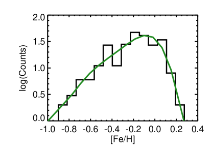
Figure 1.— Logarithmic number of stars versus logarithmic metallicity bin. The black histogram displays the distribution of metallicities in the Casagrande et al. (2008) sample and the green line is our adopted metallicity prior.

2.3. Assessing Covariance Between Fitted Parameters

Our procedure for estimating stellar parameters expressly considers the covariance between fitted parameters by simultaneously determining the likelihood of each of the models and determining the range of temperatures, metallicities, and radii that would encompass the full 68.3% confidence interval. The provided error bars therefore account for the fact that high-metallicity warm M dwarfs and low-metallicity cool M dwarfs have similar colors.

We confirm that the quoted errors on the stellar parameters are large enough to account for the errors in the photometry by conducting a perturbation analysis in which we create 100 copies of each of the Kepler M dwarfs and add Gaussian distributed noise to the photometry based on the reported uncertainty in each band. We then run our stellar parameter determination pipeline and compare the distribution of best-fit parameters for each star to our original estimates. We find that there is a correlation between higher temperatures and higher metallicities, but that our reported error bars are larger than the standard deviation of the best-fit parameters.

2.4. Validating Methodology

We confirm that we are able to recover accurate parameters for low mass stars from photometry by running our stellar parameter determination pipeline on a sample of stars with known distances. We obtained a list of 438 M dwarfs with measured parallaxes, $JHK$ photometry from 2MASS, and $g^{\prime}r^{\prime}i^{\prime}$ photometry from the AAVSO Photometric All-Sky Survey (APASS) from Jonathan Irwin (personal communication, January 2, 2013) and performed a series of quality cuts on the sample. We removed stars with parallax errors above 5% and and stars with fewer than two measurements in the APASS database. We then visually inspected the 2MASS photometry of the remaining 230 stars to ensure that none of them belonged to multiple systems that could have been unresolved in APASS and resolved in 2MASS. We removed 203 stars with other stars or quasars within 1’, resulting in a final sample of 26 stars.

We estimate the masses of the 26 stars by running our stellar parameter determination pipeline to match the observed colors to the colors of Dartmouth model stars. The APASS $g^{\prime}r^{\prime}i^{\prime}$ photometry was acquired using filters matching the original SDSS $g^{\prime}r^{\prime}i^{\prime}$ bands; we convert the APASS photometry to the unprimed SDSS 2.5m $gri$ bands using the transformation equations provided on the SDSS Photometry White Paper. We then compare the masses assigned by our pipeline to the masses predicted from the empirical relation between mass and absolute $Ks$ magnitude (Delfosse et al., 2000). As shown in Figure 2, our mass estimates are consistent with the mass predicted by the Delfosse relation. The masses predicted by the pipeline are typically $5\%$ lower than the mass predicted by the Delfosse relation, but none of these stars have reported $z$-band photometry whereas 96% of our final sample of Kepler M dwarfs have full $grizJHK$ photometry. Accordingly, we do not fit for a correction term because the uncertainty introduced by adding a scaling term based on fits made to stars with only five colors would be comparable to the offset between our predicted masses and the masses predicted by the Delfosse relation.

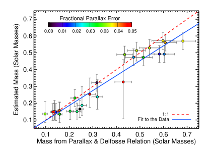
Figure 2.— Mass estimated by our photometric stellar parameter determination pipeline versus mass predicted by the Delfosse relation. The dashed red line indicates a 1:1 relation and the solid blue line is fit to the data. The points are color-coded by the reported fractional error in the parallax measurement.

3. Revised Stellar Properties

Our final sample of cool Kepler target stars includes 3897 stars with temperatures below 4000K and surface gravities above $\log g=3.6$. The sample consists primarily of late-K and early-M dwarfs, but 201 stars have revised temperatures between $3122-3300$K. The revised parameters for all of the cool dwarfs are provided in the Appendix in Table 4 Revised Cool Star Properties. We exclude 4420 stars from the final sample because their photometry is consistent with classification as evolved stars ($\log g<3.6$) and 608 stars because their photometry is insufficient to discriminate between dwarf and giant models. We refer to the stars that could be fit by either dwarf or giant models as ‘‘ambiguous’’ stars. The majority (80%) of the stars classified as ‘‘ambiguous’’ were not assigned temperatures in the KIC. We find that $96-98$% of cool bright ($T_{\mathrm{eff}}<4000$K, Kepmag $<14$) stars and $5-6$% of cool faint ($T_{\mathrm{eff}}<4000$K, Kepmag $>14$) stars are giants, which is consistent with Mann et al. (2012). (The precise fractions of giant stars depend on whether the ambiguous stars are counted as giant stars.) One of the excluded ambiguous stars is KID 8561063 (KOI 961), which was confirmed by Muirhead et al. (2012b) as a $0.17\pm 0.04{\rm\,R_{\odot}}$, $3200\pm 65$K star hosting sub-Earth-size three planet candidates. The KIC does not include $z$-band photometry for KOI 961 and we were unable to rule out matches with giant stars using only $griJHK$ photometry.

The distributions of temperature, radius, metallicity, and surface gravity for the stars in our sample are shown in Figure 3. For comparison, we display both fits made without using priors (left panels) and fits including priors on the stellar metallicity distribution and the height of stars above the plane of the galaxy (right panels). In both cases the radii of the majority of stars are significantly smaller than the values given in the KIC and the surface gravities are much higher. As discussed in Section 2.2.1, the primary difference between the two model fits is that setting a prior on the underlying metallicity distribution reduces the number of stars with revised metallicities below [Fe/H]$=-0.6$. Since such stars should be relatively uncommon, we choose to adopt the stellar parameters given by fitting the stars assuming priors on metallicity and height above the plane.

Incorporating priors, the median temperature of a star in the sample is 3723K and the median radius is $0.45{\rm\,R_{\odot}}$. Most of the stars in the sample are slightly less metal-rich than the Sun (median [Fe/H]=$-0.1$), but 21% have metallicities $0.0\leq$[Fe/H]$<0.5$. Although nearly all of the stars in the sample (96%) had KIC surface gravities below $\log g=4.7$, our reanalysis indicates that 95% actually have surface gravities above $\log g=4.7$. As shown by the purple histograms in each of the panels, the distribution of stellar parameters for the planet candidate host stars matches the overall distribution of stellar parameters for the cool star sample.

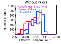
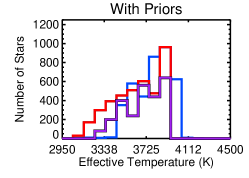
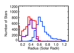
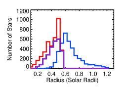
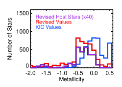
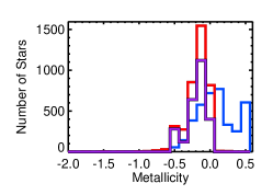
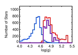
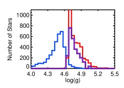
Figure 3.— Histograms of the resulting temperature (top), radius (second from top), metallicity (third from top), and surface gravity (bottom) distributions for the target stars with revised temperatures below 4000K. The panels on the left show the distributions resulting from fitting the stars without setting priors while the stellar parameters in the right panels were fit assuming priors on metallicity and height above the plane. In all panels, a histogram of the original KIC values is shown in blue and a histogram of the revised values is plotted in red. The distribution of cool host stars (multiplied by forty) is shown in purple in all plots.

The two-dimensional distribution of radii and temperatures for our chosen model fit is shown in Figure 4. The spread in the radii of the model points at a given temperature is due to the range of metallicities allowed in the model suite. At a given temperature, the majority of the original radii from the KIC lie above the model grid in a region of radius--temperature space unoccupied by low-mass stars. The discrepancy between the model radii and the KIC radii is partially due to the errors in the assumed surface gravities. As shown in Figure 3, the surface gravities assumed in the KIC peak at $\log(g)=4.5$ with a long tail extending to lower surface gravities whereas the minimum expected surface gravity for cool stars is closer to $\log(g)=4.7$.

For a typical cool star, we find that the revised radius is only $69\%$ of the original radius listed in the KIC and that the revised temperature is 130K cooler than the original temperature estimate. The majority (96%) of the stars have revised radii smaller than the radii listed in the KIC and 98% of the stars are cooler than their KIC temperatures. The revised radius and temperature distribution of planet candidate host stars is similar to the underlying distribution of cool target stars. The median changes in radius and temperature for a cool planet candidate host star are $-0.19{\rm\,R_{\odot}}$ ($-29$%) and $-102$K, respectively.

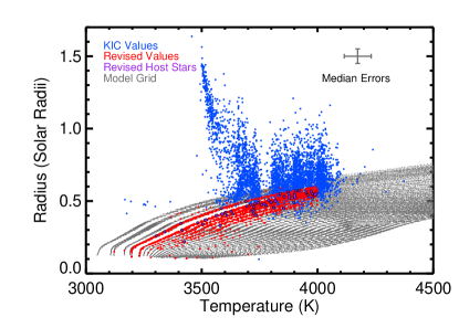
Figure 4.— Revised (red) and original (blue) temperatures and radii of the cool target stars. The revised values were determined by comparing the observed colors of stars to the expected colors of Dartmouth model stars (gray) and incorporating priors on the metallicity and height above the galactic plane. The revised stellar parameters for cool planet candidate host stars are highlighted in purple. The position of the KIC radii well above the model grid indicates that many of the combinations of radius and temperature found in the KIC are nonphysical.

We compare the revised and initial parameters for the host stars in more detail in Figure 5. For all host stars except for KOI 1078 (KID 10166274), the revised radii are smaller than the radii listed in the KIC and the revised temperatures for all of the stars are cooler than the KIC temperatures. Unlike the original values given in the KIC, the revised temperatures and radii of the cool stars align to trace out a main sequence in which smaller stars have cooler temperatures by construction.

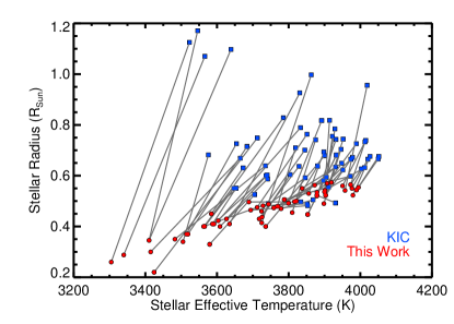
Figure 5.— Revised (red circles) and original (blue squares) radii and temperatures for the planet candidate host stars with revised temperatures below 4000K. The gray lines connect the initial and final values for each host star.

3.1. Comparison to Previous Work

We validate our revised parameters by comparing our photometric effective temperatures for a subset of the cool target stars to the spectroscopic effective temperatures from Muirhead et al. (2012a) and Mann et al. (2012). We exclude the stars KIC 5855851 and KIC 8149616 from the comparison due to concerns that their spectra may have been contaminated by light from another star (Andrew Mann, personal communication, January 15, 2013). As shown in Figure 6, our revised temperatures are consistent with the literature results for stars with revised temperatures below 4000K, which is the temperature limit for our final sample.

At higher temperatures, we find that our temperatures are systematically hotter than the literature values reported by Muirhead et al. (2012a). The temperatures given in Muirhead et al. (2012a) are determined from the H₂O-K2 index (Rojas-Ayala et al., 2012), which measures the shape of the spectrum in $K$-band. Although the H₂O-K2 index is an excellent temperature indicator for cool stars, the index saturates around 4000K, accounting for the disagreement between our temperature estimates and the Muirhead et al. (2012a) estimates for the hotter stars in our sample.

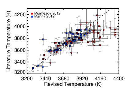
Figure 6.— Spectroscopic effective temperatures from Muirhead et al. (2012a) (red circles) and Mann et al. (2012) (blue squares) versus our revised photometric effective temperature estimates. The dashed black line indicates a 1:1 relation. The disagreement for the hotter stars is attributed to the saturation of the H₂O-K2 index used by Muirhead et al. (2012a) at temperatures above 4000K.

We also compare our photometric metallicity estimates to the spectroscopic metallicity estimates from Muirhead et al. (2012a). Given the disagreement between our temperature estimates and Muirhead et al. (2012a) at higher temperatures, we choose to plot only the 32 stars with revised temperatures below 4000K and spectroscopic metallicities from Muirhead et al. (2012a). The top panel of Figure 7 compares our revised metallicities to the spectroscopic metallicities from Muirhead et al. (2012a). We observe a systematic offset in metallicity with our values typically 0.17 dex lower than the metallicities reported in Muirhead et al. (2012a).

The metallicity difference is dependent on the spectroscopic metallicity of the star, as depicted in the lower panel of Figure 7, which shows the metallicity difference as a function of the metallicity reported in Muirhead et al. (2012a). For stars with Muirhead et al. (2012a) metallicities between -0.2 and -0.1 dex, our revised metallicities are $0.05$ dex lower, but for stars with Muirhead et al. (2012a) metallicities above 0.1 dex, our revised metallicities are 0.3 dex lower.

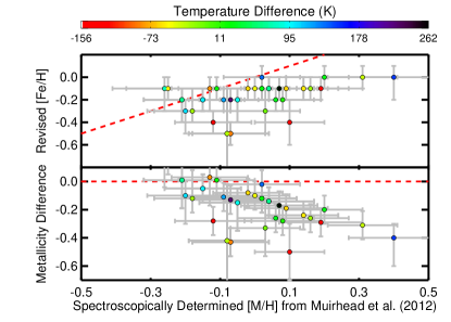
Figure 7.— Comparison of our photometric metallicity estimates to the spectroscopic metallicities from Muirhead et al. (2012a) for stars with revised $T<4000$K. The color-coding indicates our revised stellar temperatures and the dashed red lines mark a 1:1 relation between photometric and spectroscopic metallicities. Top: Revised photometric metallicity estimates versus spectroscopic metallicity. Bottom: Metallicity difference (photometric - spectroscopic) versus spectroscopic metallicity.

4. Revised Planet Candidate Properties

Our sample of cool stars includes 64 host stars with 95 planet candidates. As part of our analysis, we downloaded the Kepler photometry for the 95 planet candidates and inspected the agreement between the planet candidate parameters provided by Batalha et al. (2012) and the Kepler data. We used long cadence data from Quarters $1-6$ for all KOIs except KOI 531.01, for which we utilized short cadence data from Quarters 9 and 10 due to the range of apparent transit depths observed in the long cadence data. The long cadence data provide measurements of the brightness of the target stars every 29.4 minutes and the short cadence data provide measurements every 58.9 seconds.

We detrended the data by dividing each data point by the median value of the data points within the surrounding 1000 minute interval and masked transits of additional planets in multi-planet systems. We found that the distribution of impact parameters reported by Batalha et al. (2012) for these planet candidates was biased towards high values (median $b=0.75$) and that the published parameters for several candidates did not match the observed depth or shape. Accordingly, we used the IDL AMOEBA minimization algorithm based on Press et al. (2002) to determine the best-fit period and ephemeris for each planet candidate. We then ran a Markov Chain Monte Carlo analysis using Mandel & Agol (2002) transit models to revise the planet radius/star radius ratio, stellar radius/semimajor axis ratio, and inclination for each of the candidates. For each star, we determined the limb darkening coefficients by interpolating the quadratic coefficients provided by Claret & Bloemen (2011) for the Kepler bandpass at the effective temperature and surface gravity found in Section 2.2. We adopt the median values of the resulting parameter distributions as our best-fit values and provide the resulting planet candidate parameters in the Appendix in Table 5. Figures 8-11 display detrended and fitted light curves for the three habitable zone planet candidates in our sample and for one additional candidate at short cadence.

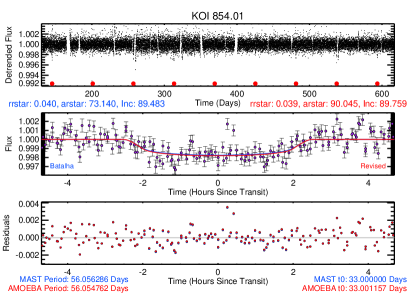
Figure 8.— Light curve for KOI 854.01. Top: Detrended light curve with transit times marked by red dots. Middle: Light curve phased to the best-fit period. The blue curve indicates the original transit model and the red curve marks our revised fit. The parameters for the fit are indicated above the middle panel and the period and ephemeris are marked at the bottom of the figure. The ‘‘MAST’’ values indicate the original period and ephemeris listed in the planet candidate list at MAST and the ‘‘AMOEBA’’ values indicate the revised period and ephemeris. Bottom: Residuals for the original transit model (blue) and our revised model (red).

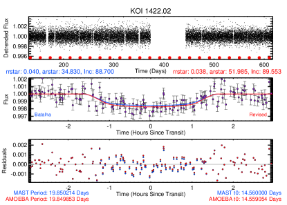
Figure 9.— Light curve for KOI 1422.02 in the same format as Figure 8.

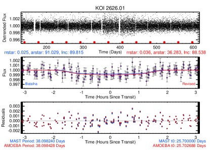
Figure 10.— Light curve for KOI 2626.01 in the same format as Figure 8.

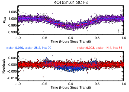
Figure 11.— Light curve for KOI 531.01. Top: Light curve phased to best-fit period. The blue curve indicates the original transit model and the red curve marks our revised fit. For clarity, only 50% of the data are plotted. The gray point in the lower right indicates representative error bars. The parameters for the fits are indicated between the panels. Bottom: Residuals for the original transit model (blue) and our revised model (red).

Ten of the planet candidates in our sample have reported transit timing variations (TTVs), but our fitting procedure assumed a linear ephemeris. Due to the smearing of ingress and egress caused by fitting a planet candidate exhibiting TTVs with a linear ephemeris, our simple fitting routine experienced difficulty determining the transit parameters for those candidates. Rather than use our poorly constrained fits for the candidates with TTVs, we choose instead to adopt the literature values for KOIs 248.01, 248.02, 886.01, and 886.02 (Kepler-49b, 49c, 54b, and 54c) from Steffen et al. (2012a), KOIs 250.01 and 250.02 (Kepler-26b and 26c) from Steffen et al. (2012b), KOIs 952.01 and 952.02 (Kepler-32b and 32c) from Fabrycky et al. (2012a), and KOIs 898.01 and 898.03 from Xie (2012).

We also adopt the transit parameters for KOIs 248.03, 248.04, and 886.03 from Steffen et al. (2012a), KOI 250.03 from Steffen et al. (2012b), KOIs 952.03 and 952.04 from Fabrycky et al. (2012a), and KOI 254.01 from Johnson et al. (2012) because the authors completed extensive modeling of their light curves. We cannot adopt values from Steffen et al. (2012b) for KOI 250.04 because that planet candidate was announced after publication of Steffen et al. (2012b). Fabrycky et al. (2012a) also present transit parameters for a fifth planet candidate in the KOI 952 system, but we choose not to add KOI 952.05 to our sample because that planet candidate was not included in the February 2012 planet candidate list (Batalha et al., 2012) and including KOI 952.05 would necessitate including any other planet candidates that were not included in the February 2012 KOI list.

For 31 of the remaining 78 planet candidates without revised fits from the literature, the planet radius/star radius ratios from Batalha et al. (2012) lie within the $1\sigma$ error bars of our revised values. The median changes to the transit parameters for the refit planet candidates are that the planet radius/star radius ratio decreases by 3%, the star radius/semimajor axis ratio increases by 18%, and the inclination increases by $0.7^{\circ}$. Combining our improved stellar radii with the revised planet radius/star radius ratios for all of the planet candidates, we find that the radius of a typical planet candidate is 29% smaller than the value found by computing the radius from the transit depth given in Batalha et al. (2012) and the stellar radii listed in the KIC as shown in Figure 12. The improvements in the stellar radii account for most of the changes in the planet candidate radii, but the contributions from the revised transit parameters are non-negligible for a few planet candidates, most notably KOIs 531.01 and 1843.02.

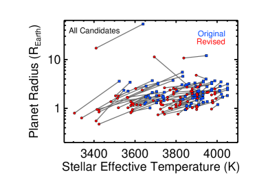
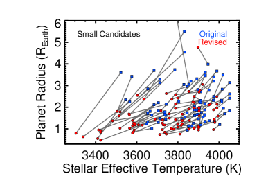
Figure 12.— Revised (red circles) and original (blue squares) planet radii and stellar effective temperatures for the 95 planet candidates. The gray lines connect the initial and final values for each planet candidate. Left: Full planet candidate population. Right: Zoomed-in view of the small planet candidate population.

We computed error bars on the planet candidate radii by computing the fractional error in the planet radius/star radius ratio and the stellar radius and adding those differences in quadrature to determine separate upper and lower $1\sigma$ error bounds for each candidate. For a typical candidate in the sample, the 68% confidence region extends from $86-112$% of the best-fit planet radius. The best-fit radii and $1\sigma$ error bars for the smallest planet candidates are plotted in Figure 13 as a function of orbital period.

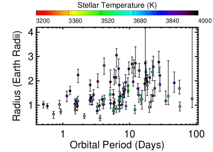
Figure 13.— Revised planet candidate radius versus orbital period for the smallest planet candidates. The points are color-coded according to the temperature of the host star.

4.1. Multiplicity

Half (48 out of 95) of our cool planet candidates are located in multi-candidate systems. We mark the multiplicity of each system in Figure 14. As shown in the figure, the largest planet candidates (KOIs 254.01, 256.01, 531.01, and 2156.01) are in systems with only one known planet and 93% of the 14 candidates with orbital periods shorter than 2 days belong to single-candidate systems. The one exception is KOI 936.02, which has an orbital period of 0.89 days and shares the system with KOI 936.01, a $1.8{\rm\,R_{\oplus}}$ planet in a 9.47 day orbit. At orbital periods longer than 2 days, 59% of the candidates belong to systems with at least one additional planet candidate. Our sample contains 47 single systems, 7 double systems, 6 triple systems, and 4 quadruple systems. The fraction of single planet systems (73%) is slightly lower than the 79% single system fraction for the planet candidates around all stars (Fabrycky et al., 2012b), but this difference is not significant.

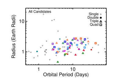
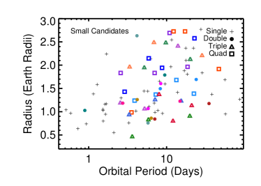
Figure 14.— Revised planet candidate radii versus orbital period for candidates in single (cross), double (circle), triple (triangle), and quadruple (square) systems. Each multi-candidate system is plotted in a different color. Left: Full planet candidate population. Right: Zoomed-in view of the smallest planet candidates.

5. Planet Occurrence Around Small Stars

We estimate the planet occurrence rate around small stars by comparing the number of detected planet candidates with the number of stars searched. Our analysis assumes that all 64 of the planet candidates are bona fide planet candidates and not false positives. This assumption is reasonable because previous studies have demonstrated that the false positive rate is low for the planet candidates identified by the Kepler team (Morton & Johnson, 2011; Fressin et al., 2013).

For a planet with a given radius and orbital period, we calculate the number of stars searched by determining the depth $\delta$ and duration of a transit in front of each of the cool stars. We then calculate the signal-to-noise ratio for a single transit of each of the stars by comparing the predicted transit depth to the expected noise level:

$${\rm SNR}_{\rm 1\,transit}=\frac{\delta}{\sigma_{\rm CDPP}}$$ (2)

where $\sigma_{\rm CDPP}$ is a measure of the expected noise on the timescale of the predicted transit duration and the depth $\delta$ for a central transit is the square of the planet/star radius ratio.

We determine $\sigma_{\rm CDPP}$ by fitting a curve to the observed Combined Differential Photometric Precision (CDPP; Christiansen et al. 2012) measured for each star over 3-hr, 6-hr, and 12-hr time periods and then interpolating to find the expected CDPP for the predicted transit duration. CDPP is available from the data search form on the Kepler MAST.

Although the CDPP varies on a quarter-by-quarter basis, we choose to interpolate the median CDPP value at a given time period for each star across all quarters. We also repeat our analysis using the minimum and maximum CDPP for each time interval to quantify the dependence of the planet occurrence rate on our estimate of the noise in the light curve on the timescale of a transit.

We then estimate the number of transits $n$ that would have been observed by dividing the number of days the star was observed by the orbital period of the planet. We assume that the total signal-to-noise scales with the number of transits so that the total signal-to-noise for a planet with radius $R_{p}$ orbiting a star with radius $R_{*}$ is:

$${\rm SNR}_{\rm total}={\rm SNR}_{\rm 1\,transit}\sqrt{n}=\left(\frac{R_{p}}{R_{*}}\right)^{2}\frac{\sqrt{n}}{\sigma_{\rm CDPP}}$$ (3)

where $n$ is the number of transits. We adopt the $7.1\sigma$ detection threshold used by the Kepler team and require that the total SNR is above 7.1$\sigma$ in order for a planet to be detected. We apply this cut both to our detected sample of planet candidates and to the sample of stars searched.

5.1. Correcting for Incomplete Phase Coverage

Previous research on the occurrence rate of planets around Kepler target stars has assumed that all stars were observed continuously during all quarters. This assumption is reasonable for the objects in the 2011 planet candidate list, but the failure of Module 3 on January 9, 2010 (Batalha et al., 2012) means that 20% of Kepler’s targets fall on a failed module every fourth quarter. In addition, some targets fall in the gaps between the modules and are observed only 1-3 quarters per year even though they never fall on Module 3.

We account for the missing phase coverage by determining the modules on which each of the stars fall during each quarter and calculating the fraction of Q1--Q6 that each star spent within the field-of-view of the detectors. For a star that spends $x$ days of the 486.5 day Q1--Q6 observation period in the field-of-view of the detectors, we assume that $x/486.5$ of transits would be present in the data. Note that our approach does not account for gaps in phase coverage during each quarter due to planned events and spacecraft anomalies. We also ignore the temporal spacing of transits relative to the gaps in phase coverage. This effect is negligible for transits that occur multiple times per quarter (i.e., durations $<90$ days), but the timing becomes important for transits that occur with periods equal to or longer than the duration of a quarter.

5.2. Calculating the Occurrence Rate

Following Howard et al. (2012), we estimate the planet occurrence rate $f$ as a function of planet radius and orbital period by dividing the number of planet candidates found with a given radius and period by the number of stars around which those candidates could have been detected. We account for non-transiting geometries by multiplying the number of planet candidates found by the inverse of the geometric likelihood $p_{\rm transit}=R_{*}/a$ that a planet with semi-major axis $a$ would appear to transit a star with radius $R_{*}$. The planet occurrence rate over a given period and planet radius range is therefore:

$$f(R_{p},P)=\sum_{i=1}^{N_{p}(R_{p},P)}{\frac{a_{i}}{R_{*,i}N_{*,i}}}$$ (4)

where $N_{p}(R_{p},P)$ is the number of planets with the radius $R_{p}$ and orbital period $P$ within the desired intervals, $a_{i}$ is the semimajor axis of planet $i$ , $R_{*,i}$ is the radius of the host star of planet $i$, and $N_{*,i}$ is the number of stars around which planet $i$ could have been detected. Like Howard et al. (2012), we estimate the error on the planet occurrence rate $f(R,p)$ by computing the binomial probability distribution of finding $N_{p}(R_{p},P)$ planets in a given radius and period range when searching $N_{p}(R_{p},P)/f(R_{p},P)$ stars. We determine the 15.9 and 84.1 percentiles of the cumulative binomial distribution and adopt those values as the 1$\sigma$ statistical errors on the occurrence rate $f(R_{p},P)$ within the desired radius and period range.

Table 1Planet Occurrence Rate for Late K and Early M Dwarfs

$0.5-0.7$ & $0.014^{+0.0129}_{-0.006}$ (2) --- $0.014^{+0.0129}_{-0.006}$ (2)
$0.7-1.0$ $0.109^{+0.0344}_{-0.025}$ (12) $0.103^{+0.0977}_{-0.046}$ (2) $0.212^{+0.0590}_{-0.044}$ (14)
$1.0-1.4$ $0.108^{+0.0251}_{-0.020}$ (21) $0.177^{+0.0735}_{-0.048}$ (7) $0.285^{+0.0509}_{-0.041}$ (28)
$1.4-2.0$ $0.080^{+0.0245}_{-0.018}$ (13) $0.123^{+0.0490}_{-0.034}$ (8) $0.202^{+0.0443}_{-0.035}$ (21)
$2.0-2.8$ $0.038^{+0.0168}_{-0.011}$ (7) $0.148^{+0.0456}_{-0.033}$ (12) $0.186^{+0.0440}_{-0.034}$ (19)
$2.8-4.0$ $0.005^{+0.0081}_{-0.003}$ (1) --- $0.005^{+0.0081}_{-0.003}$ (1)
$4.0-5.7$ $0.004^{+0.0062}_{-0.002}$ (1) --- $0.004^{+0.0062}_{-0.002}$ (1)
$5.7-8.0$ --- --- ---
$8.0-11.3$ $0.003^{+0.0044}_{-0.001}$ (1) --- $0.003^{+0.0044}_{-0.001}$ (1)
$11.3-16.0$ $0.004^{+0.0055}_{-0.002}$ (1) --- $0.004^{+0.0055}_{-0.002}$ (1)
$16.0-22.6$ $0.003^{+0.0041}_{-0.001}$ (1) --- $0.003^{+0.0041}_{-0.001}$ (1)
$22.6-32.0$ --- --- ---

Note. — The number of planets in each bin is given in parentheses.

5.3. Dependence on Planet Size

Our final sample of planet candidates orbiting dwarf stars with revised temperatures below 4000K consists of 47 candidates with radii between $0.5-1.4{\rm\,R_{\oplus}}$, 43 candidates with radii between $1.4-4{\rm\,R_{\oplus}}$, 4 candidates with radii above $4{\rm\,R_{\oplus}}$, and 1 candidate smaller than $0.5{\rm\,R_{\oplus}}$. Using Equation 4, we find the occurrence rate of planets with periods shorter than 50 days peaks at 0.29 planets per star for planets with radii between $1.0-1.4{\rm\,R_{\oplus}}$ and decreases for smaller and larger planets. We summarize our findings for the occurrence rate as a function of planet radius and orbital period in Table 5.2 and in Figure 15. Our estimate for the occurrence rate of planets with radii between $0.5-4{\rm\,R_{\oplus}}$ and orbital periods shorter than 50 days is $0.90^{+0.04}_{-0.03}$ planets per star, which agrees well with the estimate of $1.0^{+0.1}_{-0.1}$ planets per star calculated by Swift et al. (2013).

We find that the planet occurrence rate per logarithmic bin increases with increasing orbital period and that the occurrence rate of small ($R_{P}<2.8{\rm\,R_{\oplus}}$) candidates with periods less than 50 days is higher than the occurrence rate of larger candidates. The sample includes only three candidates smaller than $0.7{\rm\,R_{\oplus}}$, but the low number of planet candidates smaller than $0.7{\rm\,R_{\oplus}}$ is likely due to incompleteness in the planet candidate list and the inherent difficulty of detecting small planets. In contrast, the scarcity of planet candidates larger than $2.8~{}{\rm\,R_{\oplus}}$ indicates that large planets rarely orbit small stars at periods shorter than 50 days.

In order to more closely investigate the dependence of the planet occurrence rate on orbital period and planet radius, we plot the occurrence rate as a function of planet radius for planet candidates in three different period groups in Figure 16. For the population of candidates with periods shorter than 50 days, we find that the occurrence rate is highest for planets with radii between $1-1.4{\rm\,R_{\oplus}}$ and decreases at smaller and larger radii. The occurrence rate falls to nearly zero for planets larger than $2.8{\rm\,R_{\oplus}}$ and to 0.014 planets per star for planets with radii between $0.5-0.7{\rm\,R_{\oplus}}$. The occurrence rate of planets smaller than $0.7{\rm\,R_{\oplus}}$ might be underestimated due to incompleteness in the Kepler pipeline or there might be a real turnover in the underlying planet radius distribution at small radii.

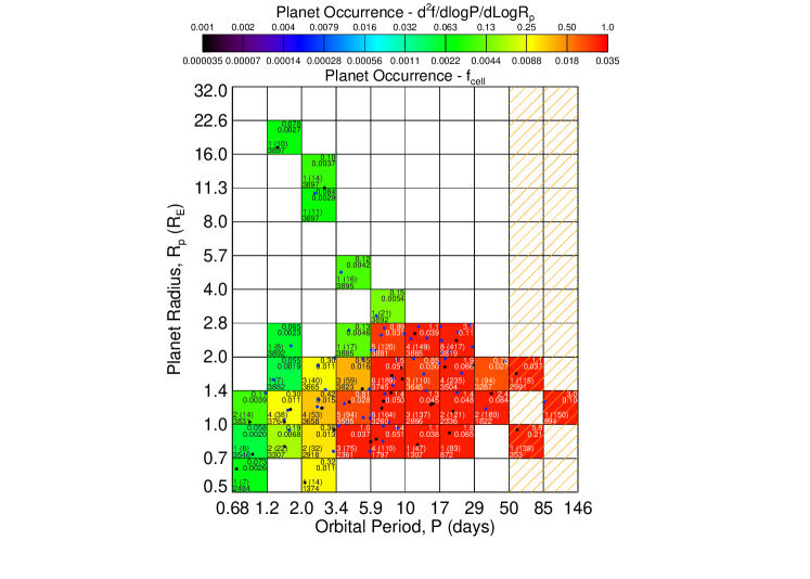
Figure 15.— Planet occurrence rate as a function of planet radius and orbital period in the style of Figure 4 from Howard et al. (2012). The color-coding of each cell indicates the planet occurrence within the cell as shown in the legend and the circles mark the radii and periods of the 95 planet candidates in our sample. Planets marked in blue orbit stars hotter than $3723$K and planets marked in black orbit stars cooler than $3723$K. Cells shaded in white do not contain any planet candidates. The planet candidate list is less complete at long periods and our estimates of the planet occurrence rate are likely underestimated at periods longer than 50 days (hatched region). The four numbers within each cell describe the planet occurrence in that region of parameter space: Top Left: number of detected planet candidates with signal to noise ratios above $7.1\sigma$ and, in parentheses, the number of non-transiting planets in the same period and radius bin computed by correcting for the geometric probability of transit; Bottom Left: the number of stars around which a planet from the center of the grid cell would have been detected with a signal to noise ratio above $7.1\sigma$; Bottom Right: the planet occurrence rate within the cell; Top Right: planet occurrence per logarithmic area unit.

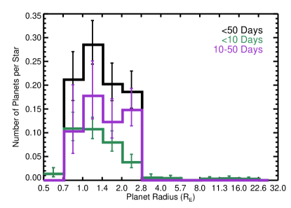
Figure 16.— Planet occurrence rate as a function of planet radius for all candidates (black) and candidates with orbital periods shorter than $<10$ days (green) or between $10-50$ days (purple). The error bars indicate the errors from binomial statistics and do not include errors from the stellar and planetary radius estimates.

Breaking down the sample by orbital period, we find a slight indication that the planet radius distribution of short-period planets ($P<10$ days) is more peaked toward smaller planet radii than the distribution of longer-period planets ($10<P<50$ days), but the difference in the occurrence rate is significant only for $2.0-2.8{\rm\,R_{\oplus}}$ planets. Our result for the occurrence rate of $2-4{\rm\,R_{\oplus}}$ planets within 50 days is 19${}^{+5}_{-4}$%, which is consistent with the $26^{+8}_{-9}$% occurrence rate for $2-4{\rm\,R_{\oplus}}$ planets found by Howard et al. (2012) for target stars with $3600\leq T_{\rm eff}\leq 4100$K. Our result is slightly below the $37\pm 8$% occurrence rate for $2-32{\rm\,R_{\oplus}}$ planets orbiting $3400\leq T_{\rm eff}\leq 4100$ stars found by Mann et al. (2012) and the 30% occurrence rate for $R_{\rm p}\geq 2{\rm\,R_{\oplus}}$ and $3660\leq T_{\rm eff}\leq 4660$K found by Gaidos et al. (2012). Howard et al. (2012) and Gaidos et al. (2012) adopt the KIC parameters for the target stars, so they overestimate both the stellar radii and planetary radii for the coolest stars in their sample. Accordingly, many of the planets that we classify as Earth-size would have ended up with radii above $2{\rm\,R_{\oplus}}$ in the Howard et al. (2012) and Gaidos et al. (2012), and studies, therefore increasing the apparent occurrence rate of $2-4{\rm\,R_{\oplus}}$ planets in those studies.

Additionally, Gaidos et al. (2012) arrive at their occurrence rate by comparing the number of planet candidates with radii between $2-32{\rm\,R_{\oplus}}$ to the number of stars around which such planets could have been detected, but they use the noise relation and distribution from Koch et al. (2010) to predict the expected noise of each star based on Kepler magnitude rather than using the observed noise. Given that the stellar noise displays variation even at constant Kepler magnitude, this assumption could contribute to the slight difference between our occurrence rate and the value reported by Gaidos et al. (2012).

Despite the sensitivity of Kepler to giant planets orbiting small stars, we find only four planets with radii $>4{\rm\,R_{\oplus}}$ in our sample (KOIs 254.01, 256.01, 531.01, and 2156.01). The implied low occurrence rate of giant planets is consistent with previous estimates of the giant planet occurrence rate around cool stars (Butler et al., 2004; Bonfils et al., 2006; Butler et al., 2006; Endl et al., 2006; Johnson et al., 2007; Cumming et al., 2008; Bonfils et al., 2011; Howard et al., 2012). The paucity of giant planets orbiting M dwarfs is in line with expectations from theoretical studies of planet formation (Laughlin et al., 2004; Adams et al., 2005; Ida & Lin, 2005; Kennedy & Kenyon, 2008). The formation of a giant planet via core accretion requires a considerable amount of material and the combination of longer orbital timescales and lower disk surface density decreases the likelihood that a protoplanet will accrete enough material to become a gas giant before the disk dissipates.

As an alternative to determining the mean number of planets per star, we also compute the fraction of stars with planets. The latter number is more relevant when determining the required number of targets to survey in a planet finding mission. To compute the fraction of stars that host planets, we repeat the analysis described in Section 5.2 using only one planet per system. We pick the planet used for each system by determining which of the planets would be easiest to detect. We find that $25\%$ of cool dwarfs host planets with radii $0.5-1.4{\rm\,R_{\oplus}}$ and orbital periods shorter than 50 days and that $25\%$ of cool dwarfs host $1.4-4{\rm\,R_{\oplus}}$ planets with periods shorter than 50 days. These estimates for the fraction of stars with planets are slightly lower than the mean number of planets per star due to the prevalence of multiplanet systems.

5.4. Dependence on Stellar Temperature

The coolest planet host star (KOI 1702) in our sample has a temperature of 3305K and the hottest planet host star (KOI 739) has a temperature of 3995K. The temperature range for the entire small star sample spans 3122-4000K, with a median temperature of 3723K. Splitting the cool star population into a cool group ($3122$K$<T_{\rm eff}<3723$K) and a hot group ($3723$K$\leq T_{\rm eff}\leq 4000$K), we find that the cool star group includes 34 KOIs orbiting 25 host stars and the hot star group includes 61 KOIs orbiting 39 host stars. The cool group contains 1957 stars total and the hot group contains 1940 stars total. The multiplicity rates for the two groups are similar: 1.4 planets per host star for the cooler group and 1.6 planets per host star for the hotter group.

In order to investigate the dependence of the planet occurrence rate on host star temperature, we repeat the analysis described in Section 5 for each group separately. We find that the occurrence rates of Earth-size planets ($0.5-1.4{\rm\,R_{\oplus}}$) are consistent with a flat occurrence rate across the temperature range of our sample, but that the occurrence rate of $1.4-4{\rm\,R_{\oplus}}$ planets is higher for the hot group than for the cool group or for the full sample. The mean numbers of Earth-size planets ($0.5-1.4{\rm\,R_{\oplus}}$) and $1.4-4{\rm\,R_{\oplus}}$ planets per star with periods shorter than 50 days are $0.57_{-0.06}^{+0.09}$ and $0.61_{-0.06}^{+0.08}$ for the hot group and $0.46_{-0.06}^{+0.09}$ and $0.19_{-0.05}^{+0.07}$ for the cool group.

The lower occurrence rate of $1.4-4{\rm\,R_{\oplus}}$ planets for the cool group indicates that cooler M dwarfs have fewer $1.4-4{\rm\,R_{\oplus}}$ planets than hotter M dwarfs, but the planet occurrence rate for mid-M dwarfs is not well constrained by the Kepler data. Since Kepler is observing few mid-M dwarfs, the median temperature for the cool star group is $3520$K and only 26% of the stars in the cool group have temperatures below 3400K. The estimated occurrence rate for the cool star group is therefore most indicative of the occurrence rate for stars with effective temperatures between $3400$K and $3723$K. Further observations of a larger sample of M dwarfs with effective temperatures below $3300$K are required to constrain the planet occurrence rate around mid- and late-M dwarfs.

5.5. The Habitable Zone

The concept of a ‘‘habitable zone’’ within which life could exist is fraught with complications due to the influence of the spectrum of the stellar flux and the composition of the planetary atmosphere on the equilibrium temperature of a planet as well as our complete lack of knowledge about alien forms of life. Regardless, for this paper we adopt the conventional and naïve assumption that a planet is within the ‘‘habitable zone’’ if liquid water would be stable on the surface of the planet. For the 64 host stars in our sample, we determine the position of the liquid water habitable zone by finding the orbital separation at which the insolation received at the top of a planet’s atmosphere is within the insolation limits determined by Kasting et al. (1993) for M0 dwarfs. Kasting et al. (1993) included several choices for the inner and outer boundaries of the habitable zone. For this paper we adopt the most conservative assumption that the inner edge of the habitable zone is the distance at which water loss occurs due to photolysis and hydrogen escape (0.95 AU for the Sun) and the outer edge as the distance at which CO₂ begins to condense (1.37 AU for the Sun).

For M0 dwarfs, these transitions occur when the insolation at the orbit of the planet is $F_{\rm inner}=1.00F_{\oplus}$ and $F_{\rm outer}=0.46F_{\oplus}$, respectively, where $F_{\oplus}$ is the level of insolation received at the top of the Earth’s atmosphere. These insolation levels are $9\%$ and $13\%$ lower than the insolation at the boundaries of the G2 dwarf habitable zone because the albedo of a habitable planet is lower at infrared wavelengths compared to visible wavelengths due to the wavelength dependence of Rayleigh scattering and the strong water and CO₂ absorption features in the near-infrared. Additionally, habitable planets around M dwarfs are more robust against global snowball events in which the entire surface of the planet becomes covered in ice because increasing the fraction of the planet covered by ice decreases the albedo of the planet at near-infrared wavelengths and therefore causes the planet to absorb more radiation, heat up, and melt the ice. This is not the case for planets orbiting Sun-like stars because ice is highly reflective at visible wavelengths and because the stellar radiation peaks in the visible.

We contemplated using the analytic relations derived by Selsis et al. (2007) for the dependence of the boundaries of the habitable zone on stellar effective temperature, but the coefficients for their outer boundary equation were fit to the shape of the maximum greenhouse limit. The analytic relations derived by Selsis et al. (2007) therefore overestimate the position of the edge of the habitable zone for our chosen limit of the first condensation of CO₂ clouds. Additionally, the equations provided in Selsis et al. (2007) are valid only for $3700$K$\leq T_{\mathrm{eff}}\leq 7200$K because Kasting et al. (1993) calculated the boundaries of the habitable zone for stars with temperatures of 3700K, 5700K, and 7200K. Selsis et al. (2007) deals with the lower temperature limit by assuming that the albedo of a habitable planet orbiting a star with a temperature below 3700K is sufficiently similar to the albedo of a habitable planet orbiting a 3700K star that the insolation limits of the habitable zone are unchanged. In this paper, we extend the Selsis et al. (2007) approximation to use constant insolation limits for all of the stars in our sample. Given the uncertainties inherent in defining a habitable planet and determining the temperatures of low-mass stars, our assumption of constant insolation boundaries should not have a significant effect on our final result for the occurrence rate of rocky planets in the habitable zones of M dwarfs.

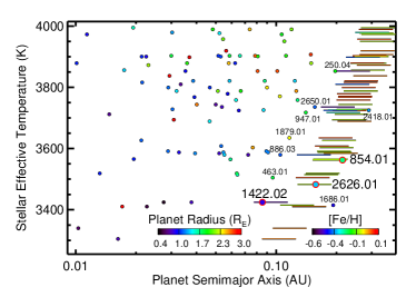
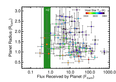
Figure 17.— Left: Stellar effective temperature and planet semimajor axes for the 95 planet candidates orbiting stars with revised temperatures below 4000K. The points are color-coded according to the radius of each planet candidate as indicated in the left legend. The lines indicate the calculated position of the habitable zone (HZ) for each star and are color-coded accorded to the metallicity of the star as indicated in the right legend. The three candidates within the HZ (KOIs 854.01, 1422.02, and 2626.01) are identified by name and highlighted in red. Right: Planet radii versus flux for the planet candidates around stars with revised temperatures below 4000K. The color-coding indicates the effective temperature of the host star. The green box indicates the habitable zone as defined in Section 5.5.

5.6. Planet Candidates in the Habitable Zone

As shown in Figure 17, the habitable zones for the 64 host stars in our final sample of dwarfs cooler than 4000K fall between 0.08 and 0.4 AU, corresponding to orbital periods of $17-148$ days. Figure 17 displays the semimajor axes of all of the planet candidates and the positions of the habitable zones around their host stars. Nearly all of the planet candidates orbit closer to their host stars than the inner boundary of the habitable zone, but two candidates (KOIs 1686.01 and 2418.01) orbit beyond the habitable zone and two candidates (KOI 250.04 and 2650.01) orbit just inside the inner edge of the habitable zone. Three candidates fall within our adopted limits: KOIs 854.01, 1422.02, and 2626.01. These candidates are identified by name in Figure 17 and have radii of 1.69, 0.92, and 1.37${\rm\,R_{\oplus}}$, respectively. A full list of the stellar and planetary parameters for the three candidates in the habitable zone and the candidates near the habitable zone is provided in Table 5.6.

The lateral variation in the position of the habitable zone at a given stellar effective temperature is due to the range of metallicities found for the host stars. At a given stellar effective temperature, stars with lower metallicities are less luminous and therefore the habitable zone is located closer to the star. Adopting a different metallicity prior would change the metallicities of the host stars and shift the habitable zones slightly inward or outward. The metallicities and temperatures of the cool stars and planet candidate host stars are plotted in Figure 18. As shown in Figure 18, 98% of the cool stars and all of the planet candidate host stars have metallicities $-0.5\leq[$Fe/H$]\leq 0$. There are 17 cool stars (0.4%) with super-solar metallicities and 75 cool stars (2%) with metallicities below [Fe/H]$=-0.5$.

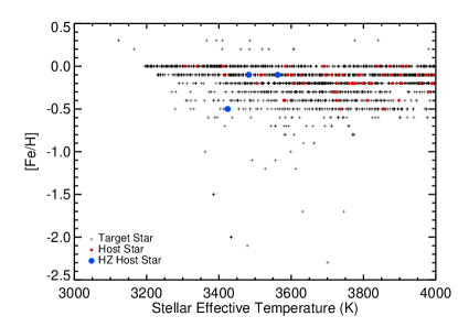
Figure 18.— Revised metallicities versus stellar effective temperature for all stars with revised temperatures below 4000K (black crosses) and planet candidate host stars (circles). The three stars hosting planet candidates within the habitable zone are highlighted in blue; all other planet host stars are marked in red.

All of the habitable zone candidates orbit stars fit by models with sub-solar metallicity (KOI 854: [Fe/H]$=-0.1$, KOI 1422: [Fe/H]$=-0.5$, KOI 2626: [Fe/H]$=-0.1$). If we restrict all of the stars to solar metallicity and redetermine the stellar parameters and habitable zone boundaries for each planet candidate, then we find that the number of candidates in the habitable zone remains constant, but that identity of the habitable zone candidates changes. KOIs 854.01 and 2626.01 remain in the habitable zone, but KOI 1422.02 does not. We find that the habitable zones of KOIs 1422 and 2418 move outward so that KOI 1422.02 is now too close to the star to be within the habitable zone and that KOI 2418.01 is now within the boundaries of the habitable zone. Because the number of candidates in the habitable zone is unchanged, our estimate of the occurrence rate within the habitable zone is not affected by adopting a different metallicity prior.

Table 2Properties of Candidates In or Near the Habitable Zone

1686.01 & 6149553 3414 0.30 -0.1 56.87 0.95 0.30
2418.01 10027247 3724 0.41 -0.4 86.83 1.27 0.35
854.01 6435936 3562 0.40 -0.1 56.05 1.69 0.50
2626.01 11768142 3482 0.35 -0.1 38.10 1.37 0.66
1422.02 11497958 3424 0.22 -0.5 19.85 0.92 0.82
250.04 9757613 3853 0.45 -0.5 46.83 1.92 1.02
2650.01 8890150 3735 0.40 -0.5 34.99 1.18 1.15
886.03 7455287 3579 0.33 -0.4 21.00 1.14 1.47
947.01 9710326 3717 0.43 -0.3 28.60 1.84 1.61
463.01 8845205 3504 0.34 -0.2 18.48 1.80 1.70
1879.01 8367644 3635 0.41 -0.2 22.08 2.37 1.96

5.7. Planet Occurrence in the Habitable Zone

Our final sample contains three planet candidates in the habitable zone, which is sufficient to allow us to place a lower limit on the occurrence rate in the habitable zone of late K and early M dwarfs. We find that planets with the same radii and insolation as KOIs 854.01, 1422.02, and 2626.01 could have been detected around 2853 (73%), 813 (21%), and 2131 (55%) of the cool dwarfs, respectively. Accordingly, the occurrence rate of Earth-size ($0.5-1.4{\rm\,R_{\oplus}}$) planets in the habitable zone is $0.15^{+0.13}_{-0.06}$  planets per star and the occurrence rate of larger ($1.4-4{\rm\,R_{\oplus}}$) planets is $0.04^{+0.06}_{-0.02}$  planets per star. We find lower limits of 0.04 Earth-size planets and $0.008$ $1.4-4{\rm\,R_{\oplus}}$ planets per cool dwarf habitable zone with 95% confidence. These occurrence rate estimates are most applicable for stars with temperatures between $3400$K and $4000$K because 80% of the stars in our cool dwarf sample have temperatures above $3400$K.

As shown in Figure 19, the occurrence rate of $1.4-4{\rm\,R_{\oplus}}$ planets peaks for insolation levels $2.2-4.7$ times higher than that received by the Earth ($F_{\oplus}$) and falls off at higher and lower insolation levels. The occurrence rate of Earth-size planets is roughly constant per logarithmic insolation bin for insolation levels between $0.2-50F_{\oplus}$ and decreases for higher levels of insolation. The large error bars at low insolation levels should shrink as the Kepler mission continues and becomes more sensitive to small planets in longer-period planets.

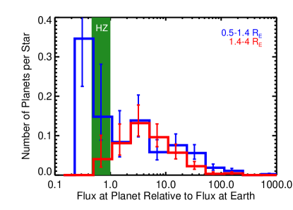
Figure 19.— Planet occurrence rate versus insolation for Earth-size planets ($0.5-1.4{\rm\,R_{\oplus}}$, blue) and $1.4-4{\rm\,R_{\oplus}}$ planets (red). The green box marks the habitable zone. The error bars indicate the errors from binomial statistics and do not include errors from the stellar and planetary radius estimates although we do consider those errors as discussed in Section 5.7.

Our result for the occurrence rate of $1.4-4{\rm\,R_{\oplus}}$ planets within the habitable zones of late K and early M dwarfs is lower than the $42^{+54}_{-13}\%$ occurrence rate reported by Bonfils et al. (2011) from an analysis of the HARPS radial velocity data. The difference between our results may be due in part to the difficulty of converting measured minimum masses into planetary radii and the definition of a ‘‘Super Earth’’ for both surveys. Small number statistics may also factor into the difference. Bonfils et al. (2011) surveyed 102 M dwarfs and found two Super Earths within the habitable zone: Gl 581c (Selsis et al., 2007; von Bloh et al., 2007) and Gl 667Cc (Anglada-Escudé et al., 2012; Delfosse et al., 2012). Their 42% estimate of the occurrence rate of Super Earths in the habitable zone includes a large correction for incompleteness. In comparison, the Kepler sample contains 3897 M dwarfs with three small habitable zone planets.

Due to the small sample size and the need to account for uncertainties in the stellar parameters, we also conduct a perturbation analysis in which we generate 10,000 realizations of each of the 3897 cool dwarfs and recalculate the occurrence rate within the habitable zone for each realization. We generate the population of cool dwarfs by drawing 10,000 model fits for each cool dwarf from the Dartmouth Stellar Models. We weight the probability that a particular model is selected by the likelihoods computed in Section 2 so that the population of models for each star represents the probability density function for the stellar parameters. For the planet host stars, we then compute the radii, semimajor axes, and insolation levels of the associated planet candidates. The full population of perturbed planet candidates is plotted in Figure 20. The realization ‘‘ellipses’’ are diagonally elongated due to the correlation between stellar temperature and radius.

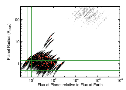
Figure 20.— Planet radii versus insolation for the population of planet candidates generated in the perturbation analysis. The best-fit parameters for each planet candidate are indicated by red circles and the perturbed realizations are marked by black points. The green lines mark the boundaries of the habitable zone as defined in Section 5.5.

For each realization of perturbed stars and associated planet candidates, we calculate the number of cool dwarfs for which each perturbed planet could have been detected. We report the median occurrence rates and the 68% confidence intervals in Table 5.7 as a function of planet radius and insolation. The estimated occurrence rates resulting from the perturbation analysis are consistent with the occurrence rates plotted in Figure 19 for the best-fit model parameters.

In addition to refining our estimate of the mean number of planets in the habitable zone, the perturbation analysis also allows us to estimate the likelihood that each of the planet candidates lies within the habitable zone. We find that the most likely habitable planet is KOI 2626.01, which lies within the habitable zone in 4,907 of the 10,000 realizations. KOIs 2650.01, 1422.02, 250.04, and 947.01 are also promising candidates and are within the habitable zone in 47%, 46%, 28%, and 22% of the realizations, respectively. KOIs 886.03, 463.01, 1686.01, 1078.03, 1879.01, 817.01, and 571.04 have much lower habitability fractions (11%, 8%, 7%, 5%, 5%, 3%, and 2%) but still contribute to the overall estimate of the occurrence rate of planets within the habitable zone of cool dwarfs.

Table 3Results of Perturbation Analysis: Planet Occurrence Rate as a Function of Flux for Late K and Early M Dwarfs

$0.10-0.21$ & --- ---
$0.21-0.46$ $0.256^{+0.210}_{-0.142}$ ---
$0.46-1.00$ $0.155^{+0.138}_{-0.098}$ $0.039^{+0.038}_{-0.039}$
$1.00-2.17$ $0.153^{+0.089}_{-0.064}$ $0.084^{+0.033}_{-0.026}$
$2.17-4.73$ $0.133^{+0.055}_{-0.043}$ $0.120^{+0.031}_{-0.030}$
$4.73-10.27$ $0.131^{+0.049}_{-0.042}$ $0.069^{+0.023}_{-0.021}$
$10.27-22.33$ $0.100^{+0.025}_{-0.023}$ $0.043^{+0.013}_{-0.011}$
$22.33-48.55$ $0.047^{+0.012}_{-0.012}$ $0.013^{+0.006}_{-0.008}$
$48.55-105.55$ $0.017^{+0.006}_{-0.006}$ $0.004^{+0.004}_{-0.001}$
$105.55-229.45$ $0.007^{+0.003}_{-0.003}$ $0.002^{+0.001}_{-0.002}$
$229.45-498.81$ $0.002^{+0.001}_{-0.002}$ ---
$498.81-1084.37$ --- ---

6. Summary and Conclusions

We update the stellar parameters for the coolest stars in the Kepler target list by comparing the observed colors of the stars to the colors of model stars from the Dartmouth Stellar Evolutionary Program. Our final sample contains 3897 dwarf stars with revised temperatures cooler than 4000K. In agreement with previous research, we find that the temperatures and radii of the coolest stars listed in the KIC are overestimated. For a typical star, our revised estimates are 130K cooler and 31% smaller. We also refit the light curves of the associated planet candidates to better constrain the planet radius/star radius ratios and combine the revised radius ratios with the improved stellar radii of the 64 host stars to determine the radii of the 95 planet candidates in our sample.

In the next stage of our analysis, we compute the planet occurrence rate by comparing the number of planet candidates to the number of stars around which Kepler could have detected planets with the same radius and orbital period or insolation. We find that the mean number of Earth-size ($0.5-1.4{\rm\,R_{\oplus}}$) planets and $1.4-4{\rm\,R_{\oplus}}$ planets with orbital periods shorter than 50 days are $0.51_{-0.05}^{+0.06}$ and $0.39_{-0.04}^{+0.05}$ planets per star, respectively. Our occurrence rate for $2-4{\rm\,R_{\oplus}}$ planets is consistent with the value reported by Howard et al. (2012) and our occurrence rate for $2-32{\rm\,R_{\oplus}}$ planets is slightly lower than the occurrence rate found by Gaidos et al. (2012).

The calculated occurrence rate of Earth-size ($0.5-1.4{\rm\,R_{\oplus}}$) planets with orbital periods shorter than 50 days is consistent with a flat occurrence rate for temperatures below 4000K, but the temperature dependence of the occurrence rate of $1.4-4{\rm\,R_{\oplus}}$ planets is significantly different. We estimate an occurrence rate of $0.61^{+0.08}_{-0.06}$ $1.4-4{\rm\,R_{\oplus}}$ planets per hotter star (3723K$\leq T_{\rm eff}\leq 4000$K) and $0.19^{+0.07}_{-0.05}$ per cooler star (3122K$\leq T_{\rm eff}<$ 3723K), noting that 74% of the stars in the cool group have temperatures between $3400$K and $3701$K. The apparent decline in the $1.4-4{\rm\,R_{\oplus}}$ planet occurrence rate at cooler temperatures might be due to the decreased surface density in the circumstellar disks of very low-mass stars and the longer orbital timescales at a given separation (Laughlin et al., 2004; Adams et al., 2005; Ida & Lin, 2005; Kennedy & Kenyon, 2008).

We also estimate the occurrence rate of potentially habitable planets around cool stars. We find that the occurrence rate of small (0.5 --1.4 ${\rm\,R_{\oplus}}$) planets within the habitable zone is $0.15^{+0.13}_{-0.06}$ planets per cool dwarf. This result is lower than the M dwarf planet occurrence rates found by radial velocity surveys (Bonfils et al., 2011), but higher than some estimates of the occurrence rate for Sunlike stars (e.g., Catanzarite & Shao, 2011). The relatively high occurrence rate of potentially habitable planets around cool stars bodes well for future missions to characterize habitable planets because the majority of the stars in the solar neighborhood are M dwarfs. Given that there are 248 early M dwarfs within 10 parsecs, we estimate that there are at least 9 Earth-size planets in the habitable zones of nearby M dwarfs that could be discovered by future missions to find nearby Earth-like planets. Applying a geometric correction for the transit probability and assuming that the space density of M dwarfs is uniform, we find that the nearest transiting Earth-size planet in the habitable zone of an M dwarf is less than $21$ pc away with 95% confidence. Removing the requirement that the planet transits, we find that the nearest non-transiting Earth-size planet in the habitable zone is within $5$ pc with 95% confidence. The most probable distances to the nearest transiting and non-transiting Earth-size planets in the habitable zone are $13$ pc and $3$ pc, respectively.

Table 4Revised Cool Star Properties

1162635 & 3759${}^{+50}_{-50}$ 0.494${}^{+0.05}_{-0.05}$ 0.505${}^{+0.05}_{-0.05}$ 4.754${}^{+0.06}_{-0.06}$ -0.10${}^{+0.1}_{-0.1}$ 261.3${}^{+17}_{-12}$
1292688 3774${}^{+77}_{-50}$ 0.530${}^{+0.07}_{-0.05}$ 0.539${}^{+0.06}_{-0.05}$ 4.722${}^{+0.06}_{-0.07}$ 0.00${}^{+0.1}_{-0.1}$ 282.1${}^{+43}_{-10}$
1293177 3385${}^{+50}_{-50}$ 0.216${}^{+0.05}_{-0.05}$ 0.204${}^{+0.05}_{-0.05}$ 5.077${}^{+0.06}_{-0.06}$ -0.40${}^{+0.1}_{-0.1}$ 101.7${}^{+15}_{-10}$
1293393 3953${}^{+137}_{-54}$ 0.536${}^{+0.13}_{-0.05}$ 0.555${}^{+0.12}_{-0.05}$ 4.725${}^{+0.06}_{-0.13}$ -0.20${}^{+0.4}_{-0.1}$ 454.2${}^{+130}_{-31}$
1429729 3903${}^{+76}_{-60}$ 0.523${}^{+0.07}_{-0.05}$ 0.541${}^{+0.07}_{-0.05}$ 4.735${}^{+0.06}_{-0.07}$ -0.20${}^{+0.2}_{-0.1}$ 380.0${}^{+61}_{-32}$
1430893 3929${}^{+98}_{-58}$ 0.541${}^{+0.07}_{-0.05}$ 0.564${}^{+0.07}_{-0.05}$ 4.724${}^{+0.06}_{-0.06}$ -0.10${}^{+0.2}_{-0.1}$ 269.8${}^{+42}_{-20}$
1433760 3296${}^{+50}_{-50}$ 0.213${}^{+0.05}_{-0.05}$ 0.196${}^{+0.05}_{-0.05}$ 5.072${}^{+0.06}_{-0.06}$ -0.10${}^{+0.1}_{-0.1}$ 109.8${}^{+13}_{-13}$
1569682 3860${}^{+93}_{-78}$ 0.514${}^{+0.06}_{-0.07}$ 0.544${}^{+0.07}_{-0.05}$ 4.752${}^{+0.07}_{-0.06}$ -0.10${}^{+0.2}_{-0.1}$ 262.8${}^{+41}_{-44}$
1569863 3591${}^{+50}_{-53}$ 0.360${}^{+0.05}_{-0.06}$ 0.384${}^{+0.07}_{-0.06}$ 4.910${}^{+0.07}_{-0.06}$ -0.30${}^{+0.1}_{-0.1}$ 157.0${}^{+25}_{-29}$
1572802 3878${}^{+53}_{-88}$ 0.535${}^{+0.05}_{-0.06}$ 0.545${}^{+0.05}_{-0.06}$ 4.719${}^{+0.06}_{-0.06}$ -0.10${}^{+0.1}_{-0.1}$ 246.4${}^{+25}_{-36}$

Note. — Table 4 Revised Cool Star Properties is published in its entirety in the electronic edition. A portion is shown here for guidance regarding its form and content.

Table 5Revised Properties for Planet Candidates Orbiting Small Stars

KOI	KID	t0 (Days)	$P$ (Days)	$a/R_{*}$	$R_{p}/R_{*}$	$b$	$R_{\rm P}({\rm\,R_{\oplus}})$	$F(F_{\oplus})$	$T_{\rm eff}(K)$	$R_{*}({\rm\,R_{\odot}})$
247.01	11852982	1.525	13.815	47.536	0.030	0.4	$1.41^{+0.26}_{-0.29}$	$4.41_{-2.95}^{+5.61}$	3725	0.437
248.01	5364071	4.593	7.028	17.897	0.032	0.6	$1.83^{+0.18}_{-0.26}$	$16.90_{-1.88}^{+3.57}$	3903	0.523
248.02	5364071	6.158	10.913	21.948	0.047	0.8	$2.69^{+0.26}_{-0.38}$	$9.40_{-6.67}^{+9.86}$	3903	0.523
248.03	5364071	2.076	2.577	10.121	0.032	0.5	$1.83^{+0.18}_{-0.26}$	$64.39_{-3.94}^{+5.83}$	3903	0.523
248.04	5364071	11.080	18.596	51.184	0.034	0.5	$1.96^{+0.19}_{-0.27}$	$4.62_{-2.14}^{+3.62}$	3903	0.523
249.01	9390653	3.871	9.549	44.353	0.040	0.3	$1.60^{+0.22}_{-0.22}$	$4.65_{-6.22}^{+7.56}$	3514	0.370
250.01	9757613	10.720	12.283	34.265	0.056	0.3	$2.73^{+0.63}_{-0.54}$	$6.06_{-3.46}^{+4.21}$	3853	0.447
250.02	9757613	11.877	17.251	62.567	0.056	0.5	$2.73^{+0.63}_{-0.54}$	$3.85_{-23.70}^{+28.82}$	3853	0.447
250.03	9757613	1.594	3.544	11.511	0.020	0.5	$0.98^{+0.23}_{-0.19}$	$31.79_{-1.70}^{+2.07}$	3853	0.447
250.04	9757613	43.087	46.828	157.259	0.039	0.6	$1.92^{+0.44}_{-0.38}$	$1.02_{-1.68}^{+2.18}$	3853	0.447
251.01	10489206	0.347	4.164	12.214	0.049	0.7	$2.63^{+0.27}_{-0.34}$	$26.00_{-15.49}^{+29.45}$	3743	0.488
251.02	10489206	0.157	5.775	18.612	0.014	0.5	$0.76^{+0.08}_{-0.10}$	$16.81_{-0.50}^{+0.94}$	3743	0.488
252.01	11187837	12.059	17.605	33.315	0.045	0.5	$2.37^{+0.25}_{-0.30}$	$3.82_{-8.78}^{+9.79}$	3770	0.479
253.01	11752906	4.643	6.383	17.910	0.049	0.8	$3.05^{+0.27}_{-0.47}$	$21.99_{-5.68}^{+6.33}$	3919	0.574
254.01	5794240	1.410	2.455	11.223	0.179	0.5	$10.74^{+0.98}_{-1.44}$	$68.37_{-1.30}^{+1.67}$	3837	0.550
255.01	7021681	24.694	27.522	51.142	0.045	0.3	$2.77^{+0.24}_{-0.34}$	$3.07_{-8.91}^{+8.92}$	3907	0.570
256.01	11548140	0.200	1.379	4.825	0.454	1.2	$17.12^{+2.48}_{-2.48}$	$49.78_{-24.90}^{+24.30}$	3410	0.346
463.01	8845205	0.491	18.478	69.231	0.049	0.5	$1.80^{+0.33}_{-0.38}$	$1.70_{-1.05}^{+1.02}$	3504	0.340
531.01	10395543	1.255	3.687	14.775	0.089	0.9	$4.77^{+0.63}_{-0.69}$	$36.55_{-18.38}^{+27.40}$	3898	0.490
571.01	8120608	7.166	7.267	22.444	0.025	0.4	$1.37^{+0.14}_{-0.21}$	$13.98_{-0.83}^{+1.36}$	3820	0.500
571.02	8120608	3.440	13.343	25.894	0.031	0.7	$1.68^{+0.17}_{-0.25}$	$6.22_{-13.83}^{+19.62}$	3820	0.500
571.03	8120608	1.184	3.887	12.801	0.023	0.6	$1.24^{+0.12}_{-0.19}$	$32.20_{-5.33}^{+6.16}$	3820	0.500
571.04	8120608	19.360	22.407	46.240	0.025	0.5	$1.39^{+0.14}_{-0.21}$	$3.12_{-2.37}^{+2.74}$	3820	0.500
596.01	10388286	0.496	1.683	8.565	0.025	0.4	$1.17^{+0.14}_{-0.16}$	$63.67_{-12.27}^{+14.19}$	3626	0.430
739.01	10386984	1.214	1.287	6.023	0.026	0.5	$1.58^{+0.19}_{-0.14}$	$187.26_{-1.19}^{+1.37}$	3994	0.554
781.01	11923270	6.418	11.598	29.230	0.055	0.7	$2.54^{+0.30}_{-0.30}$	$4.65_{-22.44}^{+28.30}$	3603	0.423
817.01	4725681	18.439	23.968	42.743	0.033	0.5	$1.69^{+0.20}_{-0.20}$	$2.45_{-50.98}^{+87.00}$	3758	0.474
817.02	4725681	3.063	8.296	45.449	0.029	0.5	$1.49^{+0.18}_{-0.17}$	$10.09_{-1.47}^{+1.99}$	3758	0.474
818.01	4913852	5.940	8.114	25.959	0.038	0.4	$1.65^{+0.21}_{-0.21}$	$6.67_{-0.78}^{+1.20}$	3564	0.401
854.01	6435936	33.001	56.055	90.045	0.039	0.4	$1.69^{+0.33}_{-0.21}$	$0.50_{-3.22}^{+4.96}$	3562	0.400
886.01	7455287	1.978	8.011	6.286	0.038	1.1	$1.38^{+0.30}_{-0.27}$	$5.30_{-2.19}^{+3.12}$	3579	0.330
886.02	7455287	10.709	12.072	6.370	0.023	1.3	$0.81^{+0.18}_{-0.16}$	$3.07_{-0.18}^{+0.35}$	3579	0.330
886.03	7455287	5.355	20.995	39.246	0.032	0.8	$1.14^{+0.25}_{-0.22}$	$1.47_{-2.48}^{+4.93}$	3579	0.330
898.01	7870390	9.615	9.770	27.672	0.042	0.4	$2.49^{+0.23}_{-0.23}$	$12.33_{-1.44}^{+2.85}$	3989	0.544
898.02	7870390	2.032	5.170	16.115	0.033	0.5	$1.96^{+0.18}_{-0.18}$	$28.81_{-0.69}^{+1.36}$	3989	0.544
898.03	7870390	7.354	20.090	41.819	0.036	0.4	$2.14^{+0.20}_{-0.20}$	$4.71_{-3.18}^{+4.32}$	3989	0.544
899.01	7907423	3.596	7.114	23.515	0.028	0.5	$1.27^{+0.15}_{-0.25}$	$8.74_{-7.43}^{+10.10}$	3587	0.410
899.02	7907423	2.114	3.307	12.885	0.021	0.4	$0.95^{+0.12}_{-0.19}$	$24.26_{-1.22}^{+1.65}$	3587	0.410
899.03	7907423	9.085	15.368	31.920	0.028	0.8	$1.24^{+0.15}_{-0.24}$	$3.13_{-4.23}^{+4.74}$	3587	0.410
936.01	9388479	7.990	9.468	27.967	0.044	0.4	$1.79^{+0.24}_{-0.26}$	$4.88_{-11.74}^{+13.16}$	3518	0.370
936.02	9388479	0.580	0.893	5.775	0.025	0.4	$1.03^{+0.14}_{-0.15}$	$113.74_{-1.51}^{+1.70}$	3518	0.370
947.01	9710326	18.333	28.599	46.796	0.039	0.7	$1.84^{+0.35}_{-0.26}$	$1.61_{-1.93}^{+2.31}$	3717	0.430
952.01	9787239	0.274	5.901	19.376	0.039	0.4	$2.15^{+0.28}_{-0.28}$	$18.06_{-44.92}^{+53.82}$	3787	0.506
952.02	9787239	4.351	8.752	19.985	0.035	0.7	$1.94^{+0.25}_{-0.26}$	$10.68_{-0.61}^{+1.16}$	3787	0.506
952.03	9787239	18.525	22.780	48.891	0.047	0.4	$2.58^{+0.33}_{-0.34}$	$2.98_{-1.10}^{+1.63}$	3787	0.506
952.04	9787239	0.400	2.896	13.641	0.026	0.5	$1.43^{+0.18}_{-0.19}$	$46.65_{-17.22}^{+25.47}$	3787	0.506
1078.01	10166274	0.720	3.354	16.129	0.035	0.4	$1.97^{+0.24}_{-0.25}$	$43.04_{-14.85}^{+21.56}$	3878	0.523
1078.02	10166274	1.417	6.877	20.830	0.044	0.9	$2.50^{+0.30}_{-0.31}$	$16.52_{-5.70}^{+8.28}$	3878	0.523
1078.03	10166274	15.729	28.463	71.424	0.039	0.5	$2.22^{+0.27}_{-0.28}$	$2.49_{-0.86}^{+1.25}$	3878	0.523
1085.01	10118816	0.219	7.718	26.930	0.018	0.6	$1.02^{+0.11}_{-0.10}$	$14.89_{-4.05}^{+6.29}$	3878	0.535
1141.01	8346392	3.424	5.728	17.940	0.024	0.5	$1.44^{+0.16}_{-0.14}$	$24.99_{-7.43}^{+10.78}$	3976	0.550
1146.01	8351704	1.504	7.097	23.314	0.019	0.4	$0.99^{+0.13}_{-0.10}$	$12.32_{-3.67}^{+5.98}$	3778	0.470
1164.01	10341831	0.780	0.934	1.768	0.014	0.3	$0.74^{+0.08}_{-0.08}$	$178.11_{-52.00}^{+68.87}$	3711	0.475
1201.01	4061149	0.690	2.758	18.588	0.023	0.4	$1.19^{+0.18}_{-0.16}$	$43.54_{-16.58}^{+27.86}$	3728	0.482
1393.01	9202151	1.164	1.695	7.709	0.037	0.4	$2.24^{+0.20}_{-0.30}$	$120.22_{-43.59}^{+41.73}$	3872	0.563
1397.01	9427402	0.829	6.247	30.153	0.036	0.4	$2.14^{+0.20}_{-0.20}$	$21.87_{-5.95}^{+8.08}$	3957	0.542
1422.01	11497958	1.568	5.842	22.474	0.035	0.4	$0.84^{+0.19}_{-0.19}$	$4.20_{-2.16}^{+3.80}$	3424	0.220
1422.02	11497958	14.559	19.850	51.985	0.038	0.4	$0.92^{+0.21}_{-0.21}$	$0.82_{-0.42}^{+0.74}$	3424	0.220
1422.03	11497958	0.743	3.622	7.933	0.020	0.9	$0.47^{+0.11}_{-0.11}$	$7.95_{-4.08}^{+7.18}$	3424	0.220
1427.01	11129738	2.463	2.613	9.757	0.023	0.5	$1.29^{+0.12}_{-0.16}$	$67.13_{-21.75}^{+25.15}$	3979	0.523
1649.01	11337141	2.239	4.044	7.983	0.019	0.9	$1.02^{+0.11}_{-0.15}$	$27.15_{-10.05}^{+11.74}$	3767	0.479
1681.01	5531953	6.486	6.939	15.493	0.027	0.8	$1.18^{+0.18}_{-0.15}$	$8.63_{-2.94}^{+4.77}$	3608	0.400
1686.01	6149553	43.529	56.867	102.482	0.029	0.5	$0.95^{+0.16}_{-0.16}$	$0.30_{-0.12}^{+0.19}$	3414	0.300
1702.01	7304449	1.082	1.538	9.008	0.028	0.6	$0.80^{+0.15}_{-0.15}$	$27.41_{-12.57}^{+20.88}$	3304	0.260
1843.01	5080636	4.103	4.195	19.152	0.026	0.4	$1.26^{+0.14}_{-0.22}$	$19.30_{-8.02}^{+9.46}$	3584	0.450
1843.02	5080636	4.025	6.356	38.543	0.018	0.5	$0.86^{+0.10}_{-0.15}$	$11.09_{-4.61}^{+5.43}$	3584	0.450
1867.01	8167996	0.033	2.550	9.819	0.022	0.5	$1.20^{+0.12}_{-0.13}$	$53.87_{-16.96}^{+24.11}$	3799	0.492
1867.02	8167996	6.446	13.969	26.759	0.045	1.0	$2.42^{+0.25}_{-0.27}$	$5.58_{-1.76}^{+2.50}$	3799	0.492
1867.03	8167996	2.404	5.212	15.672	0.020	0.5	$1.07^{+0.11}_{-0.12}$	$20.76_{-6.54}^{+9.29}$	3799	0.492
1868.01	6773862	13.183	17.761	76.082	0.034	0.4	$2.10^{+0.19}_{-0.20}$	$5.68_{-1.65}^{+2.16}$	3950	0.560
1879.01	8367644	2.731	22.085	69.891	0.053	0.5	$2.37^{+0.38}_{-0.35}$	$1.96_{-0.75}^{+1.21}$	3635	0.410
1880.01	10332883	0.847	1.151	5.801	0.024	0.7	$1.38^{+0.13}_{-0.22}$	$182.97_{-72.47}^{+69.88}$	3855	0.530
1907.01	7094486	9.197	11.350	32.483	0.033	0.5	$1.96^{+0.19}_{-0.18}$	$9.30_{-2.52}^{+3.90}$	3901	0.542
2006.01	10525027	0.233	3.273	12.574	0.015	0.5	$0.76^{+0.14}_{-0.11}$	$35.00_{-13.95}^{+23.72}$	3809	0.455
2036.01	6382217	7.635	8.411	27.409	0.028	0.4	$1.60^{+0.15}_{-0.30}$	$13.30_{-5.94}^{+6.10}$	3903	0.523
2036.02	6382217	3.489	5.795	19.205	0.019	0.6	$1.07^{+0.10}_{-0.20}$	$21.85_{-9.76}^{+10.02}$	3903	0.523
2057.01	9573685	3.200	5.945	18.668	0.019	0.5	$1.11^{+0.10}_{-0.14}$	$21.67_{-7.63}^{+7.87}$	3900	0.537
2058.01	10329835	0.575	1.524	8.046	0.018	0.5	$1.05^{+0.10}_{-0.13}$	$133.13_{-46.43}^{+47.95}$	3900	0.537
2090.01	11348997	3.845	5.132	23.462	0.027	0.4	$1.44^{+0.15}_{-0.22}$	$18.90_{-7.35}^{+8.02}$	3688	0.497
2130.01	2161536	3.445	16.855	50.586	0.031	0.4	$1.88^{+0.17}_{-0.25}$	$6.27_{-2.17}^{+2.21}$	3972	0.565
2156.01	2556650	0.835	2.852	9.813	0.223	1.2	$11.32^{+1.22}_{-1.29}$	$37.83_{-11.55}^{+14.90}$	3694	0.464
2179.01	10670119	3.851	14.871	43.731	0.027	0.4	$1.23^{+0.15}_{-0.18}$	$3.20_{-1.21}^{+1.44}$	3591	0.410
2179.02	10670119	1.564	2.733	21.112	0.026	0.5	$1.18^{+0.14}_{-0.17}$	$30.65_{-11.59}^{+13.80}$	3591	0.410
2191.01	5601258	7.441	8.848	29.479	0.019	0.6	$0.96^{+0.11}_{-0.13}$	$8.61_{-3.00}^{+4.10}$	3724	0.460
2238.01	8229458	0.313	1.647	8.090	0.016	0.5	$0.95^{+0.09}_{-0.09}$	$120.04_{-34.30}^{+38.46}$	3900	0.537
2306.01	6666233	0.040	0.512	3.419	0.018	0.5	$1.04^{+0.10}_{-0.15}$	$538.37_{-193.75}^{+219.33}$	3878	0.520
2329.01	11192235	0.326	1.615	9.104	0.021	0.6	$1.16^{+0.12}_{-0.12}$	$102.58_{-29.72}^{+41.70}$	3815	0.498
2347.01	8235924	0.352	0.588	3.717	0.016	0.4	$0.97^{+0.09}_{-0.09}$	$550.32_{-145.42}^{+187.35}$	3972	0.565
2418.01	10027247	15.600	86.830	116.837	0.028	0.5	$1.27^{+0.24}_{-0.17}$	$0.35_{-0.13}^{+0.24}$	3724	0.414
2453.01	8631751	0.235	1.531	14.100	0.024	0.5	$1.03^{+0.23}_{-0.18}$	$62.60_{-28.77}^{+57.58}$	3565	0.400
2542.01	6183511	0.000	0.727	4.643	0.020	0.4	$0.63^{+0.11}_{-0.17}$	$87.24_{-48.09}^{+74.20}$	3339	0.288
2626.01	11768142	25.703	38.098	36.283	0.036	0.9	$1.37^{+0.43}_{-0.21}$	$0.66_{-0.30}^{+0.78}$	3482	0.350
2650.01	8890150	4.280	34.987	54.052	0.027	0.5	$1.18^{+0.40}_{-0.15}$	$1.15_{-0.47}^{+1.53}$	3735	0.400
2650.02	8890150	2.155	7.054	30.813	0.019	0.5	$0.84^{+0.29}_{-0.11}$	$9.73_{-3.98}^{+12.94}$	3735	0.400
2662.01	3426367	0.742	2.104	13.578	0.015	0.5	$0.55^{+0.08}_{-0.08}$	$28.22_{-10.41}^{+16.17}$	3410	0.345

References

- Adams et al. (2005) Adams, F. C., Bodenheimer, P., & Laughlin, G. 2005, Astronomische Nachrichten, 326, 913
- Anglada-Escudé et al. (2012) Anglada-Escudé, G., Arriagada, P., Vogt, S. S., et al. 2012, ApJ, 751, L16
- Apps et al. (2010) Apps, K., Clubb, K. I., Fischer, D. A., et al. 2010, PASP, 122, 156
- Barnes et al. (2012) Barnes, J. R., Jenkins, J. S., Jones, H. R. A., et al. 2012, MNRAS, 424, 591
- Batalha et al. (2010) Batalha, N. M., Borucki, W. J, Koch, D. G., et al. 2010, ApJ, 713, L109
- Batalha et al. (2011) Batalha, N. M., Borucki, W. J., Bryson, S. T., et al. 2011, ApJ, 729, 27
- Batalha et al. (2012) Batalha, N. M., Rowe, J. F., Bryson, S. T., et al. 2012, ApJS, submitted, arXiv:1202.5852
- Berta et al. (2012) Berta, Z. K., Irwin, J., Charbonneau, D., Burke, C. J., & Falco, E. E. 2012, AJ, 144, 145
- Bonfils et al. (2011) Bonfils, X., Delfosse, X., Udry, S., et al. 2011, A&A, submitted, arXiv:1111.5019
- Bonfils et al. (2006) Bonfils, X., Delfosse, X., Udry, S., Forveille, T., & Naef, D. 2006, in Tenth Anniversary of 51 Peg-b: Status of and prospects for hot Jupiter studies, ed. L. Arnold, F. Bouchy, & C. Moutou, 111--118
- Borucki et al. (2011) Borucki, W. J., Koch, D. G., Basri, G., et al. 2011, ApJ, 736, 19
- Borucki et al. (2012) Borucki, W. J., Koch, D. G., Batalha, N., et al. 2012, ApJ, 745, 120
- Bowler et al. (2012) Bowler, B. P., Liu, M. C., Shkolnik, E. L., et al. 2012, ApJ, 753, 142
- Boyajian et al. (2012) Boyajian, T. S., von Braun, K., van Belle, G., et al. 2012, ApJ, 757, 112
- Brown et al. (2011) Brown, T. M., Latham, D. W., Everett, M. E., & Esquerdo, G. A. 2011, AJ, 142, 112
- Buccino et al. (2006) Buccino, A. P., Lemarchand, G. A., & Mauas, P. J. D. 2006, Icarus, 183, 491
- Butler et al. (2006) Butler, R. P., Johnson, J. A., Marcy, G. W., et al. 2006, PASP, 118, 1685
- Butler et al. (2004) Butler, R. P., Vogt, S. S., Marcy, G. W., et al. 2004, ApJ, 617, 580
- Casagrande et al. (2008) Casagrande, L., Flynn, C., & Bessell, M. 2008, MNRAS, 389, 585
- Castelli & Kurucz (2004) Castelli, F. & Kurucz, R. L. 2004, arXiv:astro-ph/0405087
- Catanzarite & Shao (2011) Catanzarite, J. & Shao, M. 2011, ApJ, 738, 151
- Chabrier (2003) Chabrier, G. 2003, PASP, 115, 763
- Christiansen et al. (2012) Christiansen, J. L., Jenkins, J. M., Barclay, T. S., et al. 2012, PASP, submitted, arXiv:1208.0595
- Claret & Bloemen (2011) Claret, A. & Bloemen, S. 2011, A&A, 529, A75
- Cox (2000) Cox, A. N. (ed.) 2000, Allen’s Astrophysical Quantities (New York: Springer)
- Cumming et al. (2008) Cumming, A., Butler, R. P., Marcy, G. W., et al. 2008, PASP, 120, 531
- Delfosse et al. (2012) Delfosse, X., Bonfils, X., Forveille, T., et al. 2012, A&A, submitted, arXiv:1202.2467
- Delfosse et al. (2000) Delfosse, X., Forveille, T., Ségransan, D., et al. 2000, A&A, 364, 217
- Delfosse et al. (1999) Delfosse, X., Forveille, T., Beuzit, J.-L., et al. 1999, A&A, 344, 897
- Demarque et al. (2004) Demarque, P., Woo, J.-H., Kim, Y.-C., & Yi, S. K. 2004, ApJS, 155, 667
- Dole (1964) Dole, S. H. 1964, Habitable planets for man (New York: Blaisdell Pub. Co.)
- Dotter et al. (2008) Dotter, A., Chaboyer, B., Jevremović, D., et al. 2008, ApJS, 178, 89
- Dumusque et al. (2012) Dumusque, X., Pepe, F., Lovis, C., et al. 2012, Nature, 491, 207
- Endl et al. (2006) Endl, M., Cochran, W. D., Kürster, M., Paulson, D. B., et al. 2006, ApJ, 649, 436
- Endl et al. (2003) Endl, M., Cochran, W. D., Tull, R. G., & MacQueen, P. J. 2003, AJ, 126, 3099
- Fabrycky et al. (2012a) Fabrycky, D. C., Ford, E. B., Steffen, J. H., et al. 2012a, ApJ, 750, 114
- Fabrycky et al. (2012b) Fabrycky, D. C., Lissauer, J. J., Ragozzine, D., et al. 2012b, ApJ, submitted, arXiv:1202.6328
- Feiden et al. (2011) Feiden, G. A., Chaboyer, B., & Dotter, A. 2011, ApJ, 740, L25
- Fressin et al. (2012) Fressin, F., Torres, G., Rowe, et al. 2012, Nature, 482, 195
- Fressin et al. (2013) Fressin, F., Torres, G., Charbonneau, D., et al. 2013, arXiv:1301.0842
- France et al. (2012) France, K., Froning, C. S., Linsky, J. L., et al. 2012, arXiv:1212.4833
- Gaidos et al. (2012) Gaidos, E., Fischer, D. A., Mann, A. W., & Lépine, S. 2012, ApJ, 746, 36
- Gautier et al. (2012) Gautier, III, T. N., Charbonneau, D., Rowe, J. F., et al. 2012, ApJ, 749, 15
- Giacobbe et al. (2012) Giacobbe, P., Damasso, M., Sozzetti, A., et al. 2012, MNRAS, 424, 3101
- Gilliland et al. (2011) Gilliland, R. L., Chaplin, W. J., Dunham, E. W., et al. 2011, ApJS, 197, 6
- Haberle et al. (1996) Haberle, R. M., McKay, C. P., Tyler, D., & Reynolds, R. T. 1996, in Circumstellar Habitable Zones, ed. L. R. Doyle, 29
- Hauschildt et al. (1999a) Hauschildt, P. H., Allard, F., & Baron, E. 1999a, ApJ, 512, 377
- Hauschildt et al. (1999b) Hauschildt, P. H., Allard, F., Ferguson, J., Baron, E., & Alexander, D. R. 1999b, ApJ, 525, 871
- Henry et al. (2006) Henry, T. J., Jao, W.-C., Subasavage, J. P., et al. 2006, AJ, 132, 2360
- Howard et al. (2012) Howard, A. W., Marcy, G. W., Bryson, S. T., et al. 2012, ApJS, 201, 15
- Ida & Lin (2005) Ida, S. & Lin, D. N. C. 2005, ApJ, 626, 1045
- Johnson et al. (2007) Johnson, J. A., Butler, R. P., Marcy, G. W., et al. 2007, ApJ, 670, 833
- Johnson et al. (2012) Johnson, J. A., Gazak, J. Z., Apps, K., et al. 2012, AJ, 143, 111
- Joshi et al. (1997) Joshi, M. M., Haberle, R. M., & Reynolds, R. T. 1997, Icarus, 129, 450
- Kasting et al. (1993) Kasting, J. F., Whitmire, D. P., & Reynolds, R. T. 1993, Icarus, 101, 108
- Kennedy & Kenyon (2008) Kennedy, G. M. & Kenyon, S. J. 2008, ApJ, 673, 502
- Koch et al. (2010) Koch, D. G., Borucki, W. J., Basri, G., et al. 2010, ApJ, 713, L79
- Koppen & Vergely (1998) Koppen, J. & Vergely, J.-L. 1998, MNRAS, 299, 567
- Laughlin et al. (2004) Laughlin, G., Bodenheimer, P., & Adams, F. C. 2004, ApJ, 612, L73
- Law et al. (2012) Law, N. M., Kraus, A. L., Street, R., et al. 2012, ApJ, 757, 133
- Leggett (1992) Leggett, S. K. 1992, ApJS, 82, 351
- Lépine et al. (2007) Lépine, S., Rich, R. M., & Shara, M. M. 2007, ApJ, 669, 1235
- Mandel & Agol (2002) Mandel, K. & Agol, E. 2002, ApJ, 580, L171
- Mann et al. (2012) Mann, A. W., Gaidos, E., Lépine, S., & Hilton, E. J. 2012, ApJ, 753, 90
- Morton & Johnson (2011) Morton, T. D., & Johnson, J. A. 2011, ApJ, 738, 170
- Mould & Hyland (1976) Mould, J. R., & Hyland, A. R. 1976, ApJ, 208, 399
- Muirhead et al. (2012a) Muirhead, P. S., Hamren, K., Schlawin, E., et al. 2012a, ApJ, 750, L37
- Muirhead et al. (2012b) Muirhead, P. S., Johnson, J. A., Apps, K., et al. 2012b, ApJ, 747, 144
- Nutzman & Charbonneau (2008) Nutzman, P. & Charbonneau, D. 2008, PASP, 120, 317
- Pierrehumbert (2011) Pierrehumbert, R. T. 2011, ApJ, 726, L8
- Pinsonneault et al. (2012) Pinsonneault, M. H., An, D., Molenda-Żakowicz, J., et al. 2012, ApJS, 199, 30
- Press et al. (2002) Press, W. H., Teukolsky, S. A., Vetterling, W. T., & Flannery, B. P. 2002, Numerical recipes in C++ : the art of scientific computing
- Rojas-Ayala et al. (2012) Rojas-Ayala, B., Covey, K. R., Muirhead, P. S., & Lloyd, J. P. 2012, ApJ, 748, 93
- Salpeter (1955) Salpeter, E. E. 1955, ApJ, 121, 161
- Schlaufman & Laughlin (2011) Schlaufman, K. C. & Laughlin, G. 2011, ApJ, 738, 177
- Segura et al. (2010) Segura, A., Walkowicz, L. M., Meadows, V., Kasting, J., & Hawley, S. 2010, Astrobiology, 10, 751
- Selsis et al. (2007) Selsis, F., Kasting, J. F., Levrard, B., et al. 2007, A&A, 476, 1373
- Steffen et al. (2012a) Steffen, J. H., Fabrycky, D. C., Agol, E., et al. 2012a, MNRAS, 87
- Steffen et al. (2012b) Steffen, J. H., Fabrycky, D. C., Ford, E. B., et al. 2012b, MNRAS, 421, 2342
- Swift et al. (2013) Swift, J. J., Johnson, J. A., Morton, T. D., et al. 2013, ApJ, 764, 105
- Tenenbaum et al. (2012) Tenenbaum, P., Jenkins, J. M., Seader, S., et al. 2012, ArXiv e-prints
- Traub (2012) Traub, W. A. 2012, ApJ, 745, 20
- von Bloh et al. (2007) von Bloh, W., Bounama, C., Cuntz, M., & Franck, S. 2007, A&A, 476, 1365
- Xie (2012) Xie, J.-W. 2012, ApJ, submitted, arXiv:1208.3312
- Youdin (2011) Youdin, A. N. 2011, ApJ, 742, 38
- Zechmeister et al. (2009) Zechmeister, M., Kürster, M., & Endl, M. 2009, A&A, 505, 859