The Eos family halo

Abstract

We study K-type asteroids in the broad surroundings of the Eos family because they seem to be intimately related, according to their colours measured by the Sloan Digital Sky Survey. Such ‘halos’ of asteroid families have been rarely used as constraints for dynamical studies to date. We explain its origin as bodies escaping from the family ‘core’ due to the Yarkovsky semimajor-axis drift and interactions with gravitational resonances, mostly with the 9/4 mean-motion resonance with Jupiter at 3.03 AU. Our $N$-body dynamical model allows us to independently estimate the age of the family $1.5\hbox{ to }1.9$ Gyr. This is approximately in agreement with the previous age estimate by Vokrouhlický et al. (2006) based on a simplified model (which accounts only for changes of semimajor axis). We can also constrain the geometry of the disruption event which had to occur at the true anomaly $f\simeq 120^{\circ}\hbox{ to }180^{\circ}$.

1 Introduction

The Eos family is one of the best-studied families in the main asteroid belt. Although we do not attempt to repeat a thorough review presented in our previous paper Vokrouhlický et al. (2006), we recall that the basic structure of the family is the following: (i) there is a sharp inner boundary coinciding with the 7/3 mean-motion resonance with Jupiter at approximately 2.96 AU; (ii) the 9/4 mean-motion resonance with Jupiter divides the family at 3.03 AU and asteroids with larger sizes are less numerous at larger semimajor axes; (iii) there is an extension of the family along the $z_{1}\equiv g-g_{6}+s-s_{6}$ secular resonance towards lower values of proper semimajor axis $a_{\rm p}$, eccentricity $e_{\rm p}$ and inclination $\sin I_{\rm p}$. All these fact seem to be determined by the interaction between the orbits drifting due to the Yarkovsky effect in semimajor axis and the gravitational resonances which may affect eccentricities and inclinations.

In this work, we focus on a ’halo’ of asteroids around the nominal Eos family which is clearly visible in the Sloan Digital Sky Survey, Moving Object Catalogue version 4 (SDSS, Parker et al. 2008). As we shall see below, both the ‘halo’ and the family have the same SDSS colours and are thus most likely related to each other. Luckily, the Eos family seems to be spectrally distinct in this part of the main belt (several Eos family members were classified as K-types by DeMeo et al. 2009) and it falls in between S-complex and C/X-complex asteroids in terms of the SDSS colour indices. Detailed spectroscopic observations were also performed by Zappalà et al. (2000) which confirmed that asteroids are escaping from the Eos family due to the interaction with the J9/4 resonance.

Our main motivation is to understand the origin of the whole halo and to explain its unusually large spread in eccentricity and inclination which is hard to reconcile with any reasonable initial velocity field. Essentially, this is a substantial extension of work of Vokrouhlický et al. (2006), but here we are interested in bodies which escaped from the nominal family.

We were also curious if such halos may be somehow related to the giant-planet migration which would have caused significant gravitational perturbations of all small-body populations (Morbidelli et al., 2005). Of course, in such a case the process is size-independent and moreover the age of the corresponding family would have to approach 3.9 Gyr in order to match the Nice model of giant-planet migration.

In Section 2, we define the Eos halo and core populations. Section 3 is devoted to a description of our dynamical model and to a comparison with the SDSS observations. We discuss consequences of our results in Section 4.

2 A discernment of the family core and halo

In this Section, we proceed as follows: (i) we use a hierarchical clustering method to extract the nominal Eos family; (ii) we look at the members of the family with SDSS colours and we define a colour range; (iii) we select all asteroids with Eos-like colours from the SDSS catalogue; finally, (iv) we define a halo and core using simple ’boxes’ in the proper-element space.

2.1 Colours of Eos-like asteroids

We want to select asteroids similar to the Eos family, but first we have to choose a criterion to do so. We thus identify the nominal Eos family using a hierarchical clustering method (HCM, Zappalà et al. 1995) with a suitably low cut-off velocity $v_{\rm cutoff}=50\,{\rm m}/{\rm s}$ (which leads to a similar extent of the family as in Vokrouhlický et al. (2006)), and extract colour data from the SDSS catalogue (see Figure 1). The majority of Eos-family asteroids have colour indices in the following intervals

$$a^{*} \in (0.0,0.1)\,{\rm mag}\,,$$ (1)

$$i-z \in (-0.03,0.08)\,{\rm mag}$$ (2)

which then serves as a criterion for the selection of Eos-like asteroids in the broad surroundings of the nominal family.

We also used an independent method for the selection of Eos-like asteroids employing a 1-dimensional colour index (which was used in Parker et al. 2008 to construct their colour palette) and we verified that our results are not sensitive to this procedure.

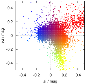
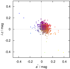
Figure 1: Colour indices $i-z$ and $a^{*}$ (defined in Parker et al. (2008)) of all asteroids from the Sloan Digital Sky Survey, Moving Object Catalogue version 4 and the corresponding colour palette (top panel) which is used in the following figures to distinguish colours of asteroids. We also plot the Eos family members observed by the SDSS (bottom panel) with small photometric uncertainties (less than 0.03 mag). The inferred range of colour indices (denoted by the dashed yellow rectangle) is then used as a criterion for the selection of the Eos-like asteroids in the broad surroundings of the nominal family. The rectangle does not encompass the outliers.

2.2 Boundaries in the proper element space

Next, we have to distinguish the family ’core’ and ’halo’ populations on the basis of proper orbital elements $(a_{\rm p},e_{\rm p},\sin I_{\rm p})$ which will be consistently used for both the SDSS observations and our dynamical models. We also need to define ’background’ population which enables to estimate how many asteroids might have Eos-like colours by chance. We decided to use a simple box criterion (see Figures 2, 3 and Table 1), while the range of proper semimajor axis is always the same, $a_{\rm p}\in(2.95,3.16)\,{\rm AU}$.

Table 1: The definitions of the core, halo and background populations in terms of intervals of proper eccentricity $e_{\rm p}$ and proper inclination $\sin I_{\rm p}$. The range of proper semimajor axis $a_{\rm p}\in(2.95,3.16)\,{\rm AU}$ is the same in all cases.

population	$e_{\rm p}$	$\sin I_{\rm p}$	note
core	0.04–0.10	0.15–0.20
halo	0.00–0.15	0.12–0.24	and not in the core
background	0.00–0.15	0.06–0.12	together with…
	0.00–0.15	0.24–0.30

Our results do not depend strongly on the selection criterion. For example, we tested a stringent definition: core was identified by the HCM at $v_{\rm cutoff}=50\,{\rm m}/{\rm s}$ and all remaining bodies in the surroundings belong to the halo. This approach makes the core as small as possible and the halo correspondingly larger but our results below (based on halo/core ratios) would be essentially the same. According to our tests, not even a different definition of the background/halo boundary changes our results.

We are now ready to construct size-frequency distributions of individual populations. In order to convert absolute magnitudes $H$ to diameters $D$ we computed the median geometric albedo $p_{V}=0.16$ from the WISE data (Masiero et al., 2011) for the nominal Eos family members. The size-frequency distribution (Figure 4) of the halo has a cumulative slope $N(>D)\propto D^{\gamma}$ equal to $\gamma=-3.9\pm 0.2$ in the size range $D=6\hbox{ to }15\,{\rm km}$ and is significantly steeper than that of the core ($\gamma=-2.2\pm 0.1$). Even this difference of slopes $(1.7\pm 0.2)$ indicates that if there a process transporting asteroids from the core to the halo it must be indeed size-dependent.

A frequency analysis similar as in Carruba and Michtchenko (2007) or Carruba (2009) shows that there is approximately 5 % of likely $z_{1}$ resonators (with the frequency $g-g_{6}+s-s_{6}<0.3\,^{\prime\prime}/{\rm yr}$) in the halo region. However, the concentration of objects inside and outside the resonance is roughly the same, so that this secular resonance does not seem to be the most important transport mechanism.

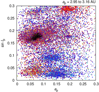
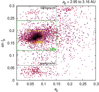
Figure 2: The proper eccentricity $e_{\rm p}$ vs proper inclination $\sin I_{\rm p}$ plot for asteroids included in the SDSS MOC 4 catalogue. The proper semimajor axis is confined to the interval 2.95 to 3.16 AU, i.e. the Eos family zone. Colour coding corresponds to the SDSS colour indices according to Figure 1. The top panel includes all asteroids (regardless of their colours). The bottom panel shows only a subset of ’Eos-like’ asteroids with colours similar to those of the Eos members (see Fig. 1, bottom). Moreover, we denote a box used for the definition of the family ’core’ (dashed yellow line) a larger box for the ’halo’ (dotted green line) and two boxes considered as ’background’ (thin black line). For comparison, we also plot positions of the nominal Eos family members (black dots), identified for the velocity $v_{\rm cutoff}=50\,{\rm m}/{\rm s}$.

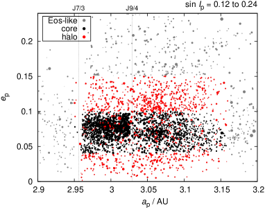
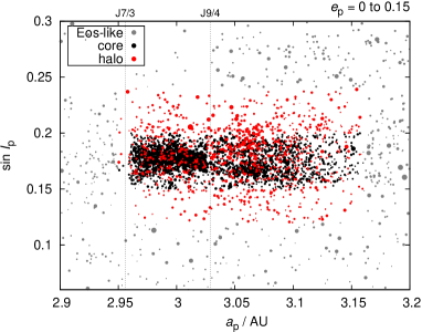
Figure 3: The proper semimajor axis $a_{\rm p}$ vs proper eccentricity $e_{\rm p}$ (top panel) and $a_{\rm p}$ vs proper inclination $\sin I_{\rm p}$ (bottom panel) for the observed Eos core (black dots), halo (red dots) and remaining Eos-like asteroids (gray dots) in the surroundings. The sizes of symbols are (inversely) proportional to the absolute magnitudes $H$ of asteroids. The positions of important mean-motion resonances with Jupiter are also indicated (dotted vertical lines).

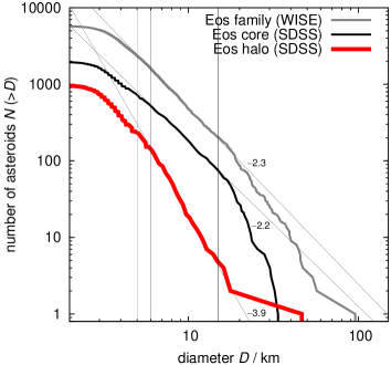
Figure 4: The cumulative size-frequency distributions $N({>}D)$ of the Eos core and halo. We show power-law fits and corresponding slopes $\gamma$ which clearly indicate that the halo population is significantly steeper than the core population. For comparison, we also plot the SFD of the nominal Eos family (as inferred from the WISE data, Masiero et al. 2011). The SFD’s of the core and halo are biased because they include only asteroids observed by the SDSS. Consequently, the core seems to be much less populated than the nominal Eos family, even though these SFD’s should be very similar. Nevertheless, the slopes and the halo/core ratios which we use in our analysis is not much affected by this bias.

3 Yarkovsky-driven origin of the halo

Motivated by the differences of the observed SFD’s, we now want to test a hypothesis that the Eos family halo (or at least a part of it) was created by the Yarkovsky semimajor-axis drift, which pushes objects from the core into neighbouring mean-motion resonances and consequently to the halo region.

3.1 Initial conditions

We prepared an $N$-body simulation of the long-term evolution of the Eos core and halo with the following initial conditions: we included the Sun and the four giant planets on current orbits. We applied a standard barycentric correction to both massive objects and test particles to prevent a substantial shift of secular frequencies (Milani and Knezevic, 1992). The total number of test particles was 6545, with sizes ranging from $D=104\hbox{ to }1.5\,{\rm km}$ and the distribution resembling the observed SFD of the Eos family.

Material properties were as follows: the bulk density $\rho=2500\,{\rm kg}/{\rm m}^{3}$, the surface density $\rho_{\rm s}=1500\,{\rm kg}/{\rm m}^{3}$, the thermal conductivity $K=0.001\,{\rm W}/{\rm m}/{\rm K}$, the specific thermal capacity $C=680\,{\rm J}/{\rm kg}/{\rm K}$, the Bond albedo $A=0.1$, the infrared emissivity $\epsilon=0.9$, i.e. all typical values for regolith covered basaltic asteroids.

Initial rotation periods were distributed uniformly on the interval 2 to 10 hours and we used random (isotropic) orientations of the spin axes. The YORP model of the spin evolution was described in detail in Brož et al. (2011), while the efficiency parameter was $c_{\rm YORP}=0.33$ (i.e. a likely value according to Hanuš et al. 2011). YORP angular momenta affecting the spin rate and the obliquity were taken from Čapek and Vokrouhlický (2004). We also included spin axis reorientations caused by collisions with a time scale estimated by Farinella et al. (1998): $\tau_{\rm reor}=B\left({\omega/\omega_{0}}\right)^{\beta_{1}}\left({D/D_{0}}\right)^{\beta_{2}}$, where $B=84.5\,{\rm kyr}$, $\beta_{1}=5/6$, $\beta_{2}=4/3$, $D_{0}=2\,{\rm m}$ and $\omega_{0}$ corresponds to period $P=5$ hours.

The initial velocity field was size-dependent, $v\propto v_{0}D_{0}/D$, with $v_{0}=93\,{\rm m}/{\rm s}$ and $D_{0}=5\,{\rm km}$ (i.e. the best-fit values from Vokrouhlický et al. 2006). In principle, this type of size–velocity relation was initially suggested by Cellino et al. (1999), but here, we attempt to interpret the structure of the family as a complex interplay between the velocity field and the Yarkovsky drift which is also inversely proportional to size. We assumed isotropic orientations of the velocity vectors. The geometry of collisional disruption was determined by the true anomaly $f=150^{\circ}$, and the argument of perihelion $\omega=30^{\circ}$. We discuss different geometries in Section 4.

We use a modified version of the SWIFT package (Levison and Duncan, 1994) for numerical integrations, with a second-order symplectic scheme (Laskar and Robutel, 2001), digital filters employing frequency-modified Fourier transform (Šidlichovský and Nesvorný, 1996) and an implementation of the Yarkovsky effect (Brož, 2006). The integration time step was $\Delta t=91\,{\rm days}$, the output time step after all filtering procedures $10\,{\rm Myr}$ and the total integration time span reached 4 Gyr.

3.2 Results of the $N$-body simulation

Initially, almost all asteroids are located in the core (see Figure 5). Only a few outliers may have velocities large enough to belong to the halo. Within a few million years the halo/core ratio quickly increases due to objects located inside the 9/4 resonance and injected to the halo by these size-independent gravitational perturbations. Further increase is caused by the Yarkovsky/YORP semimajor axis drift which pushes additional orbits into the J9/4 and also other resonances.

We checked the orbital elements of bodies at the moment when they enter the halo region (Figure 6) and we computed the statistics of dynamical routes that had injected bodies in the halo: J9/4 57 %, J11/5 (together with a three-body resonance $3{\rm J}-2{\rm S}-1$ with Jupiter and Saturn) 10 %, J7/3 6 %, and $z_{1}$ secular resonance 23 %. The remaining few percent of bodies may enter the halo by different dynamical routes. However, if we account for the fact that bodies captured by the $z_{1}$ resonance usually encounter also the J9/4 resonance that scatters them further away in to the halo, we obtain a modified statistics: J9/4 70 %, J11/5 12 %, J7/3 5 %, and $z_{1}$ 10 % that better reflects the importance of different mechanisms.

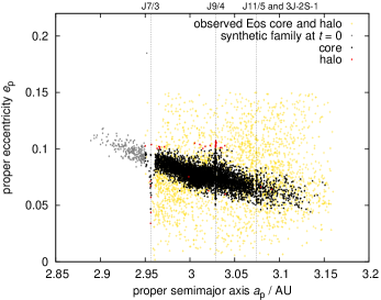
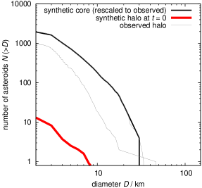
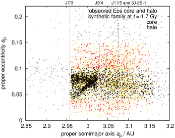
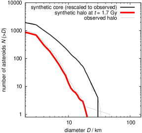
Figure 5: Left panels: the proper semimajor axis $a_{\rm p}$ vs proper eccentricity $e_{\rm p}$ plots showing a dynamical evolution of our synthetic family. We can distinguish the core (black dots), the halo (red dots) and objects beyond the halo box (gray dots). There is a comparison to the observed Eos core and halo too (yellow crosses), as inferred from the SDSS data (the same as in Figure 2, bottom). The positions of important resonances are indicated by vertical dotted lines. We plot the initial situation at $t=0$ (top panel) and the evolved family at $t=1.7$ Gyr (bottom panel). The core of the synthetic family exhibits a slightly different structure than the observed core which may indicate that: (i) the initial true anomaly was closer to $f=180^{\circ}$, or (ii) the initial velocity field deviated from the assumed $v\propto 1/D$ dependence. Right panels: the corresponding size-frequency distributions of the synthetic core (black line), which was always scaled to the observed SFD of the Eos core, and the synthetic halo (red line) which can be then directly compared to the observed halo (gray line). It is clear that the halo’s SFD becomes steeper in the course of time and at $t\simeq 1.7$ Gyr it matches the observed SFD.

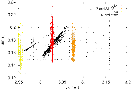
Figure 6: The proper semimajor axis $a_{\rm p}$ vs proper inclination $\sin I_{\rm p}$ of the synthetic family members at the moment when they have entered the halo region. It is easy to distinguish objects injected by mean-motion resonances and by secular resonances in this projection, because the former have a particular value of the semimajor axis. The objects injected by the J9/4 resonance are denoted by red colour, the J11/5 and $3{\rm J}-2{\rm S}-1$ by orange, the J7/3 by yellow, the $z_{1}$ secular resonance and other resonances by black.

A saturation of the halo occurs after approximately $1\,{\rm Gyr}$, because the halo population is affected by the Yarkovsky/YORP drift too, so that the injection rate roughly matches the removal rate. Nevertheless, the halo/core ratio steadily increases, which is caused by the ongoing decay of the core population.

In order to compare our model and the SDSS observations we compute the ratio ${\cal R}={{\rm d}N_{\rm halo}/{\rm d}N_{\rm core}}$ between the number of objects in the halo and in the core for a given differential size bin. This can be computed straightforwardly from our simulation data. In case of the SDSS observations, however, we think that there is a real background of asteroids with Eos-like colours (may be due to observational uncertainties or a natural spread of colours; see Figure 2). Obviously, such background overlaps with the core and the halo, so we need to subtract this contamination

$${\cal R}_{\rm obs}\equiv{{\rm d}N_{\rm halo}-0.833\,{\rm d}N_{\rm background}\over{\rm d}N_{\rm core}-0.167\,{\rm d}N_{\rm background}}\,.$$ (3)

The numerical coefficients then reflect different ’volumes’ of the halo, core and background in the space of proper elements $(a_{\rm p},e_{\rm p},\sin I_{\rm p})$, as defined in Table 1.

As we can see in Figure 7, a reasonable match to the observed halo/core ratios can be obtained for ages 1.5 Gyr (for smaller bodies) to 2.2 Gyr (for larger bodies). To better quantify the difference between the model and the observations we construct a suitable metric

$$\chi^{2}(t)\equiv\sum_{i=2}^{9}{({\cal R}_{i}(t)-{\cal R}_{{\rm obs}i})^{2}\over\sigma_{i}^{2}(t)+\sigma_{{\rm obs}i}^{2}}\,,$$ (4)

where the summation is over the respective size bins $(D_{i},D_{i}+{\rm d}D)$, $D_{i}\equiv i\cdot 1\,{\rm km}$ and ${\rm d}D=1\,{\rm km}$. The uncertainties of the numbers of objects are of the order $\sigma_{\rm halo}\simeq\sqrt{{\rm d}N_{\rm halo}}$, $\sigma_{\rm core}\simeq\sqrt{{\rm d}N_{\rm core}}$, and $\sigma_{i}$ reflects their propagation during the calculation of the ratio in Eq. (3) in a standard way

$$\sigma_{i}=\sqrt{(\sigma_{\rm halo}/{\rm d}N_{\rm halo})^{2}+(\sigma_{\rm core}/{\rm d}N_{\rm core})^{2}}\,{{\rm d}N_{\rm halo}/{\rm d}N_{\rm core}}$$

and similarly for $\sigma_{{\rm obs}i}$. The $\chi^{2}(t)$ dependence is shown in Figure 7 and the best-fit is obtained again for the ages $t\simeq 1.5\hbox{ to }2.2\,{\rm Gyr}$.

The ratios ${\cal R}$ are directly related to the size-frequency distributions and consequently we are indeed able to match the observed SFD’s of halo and core, including their slopes and absolute numbers (Figure 5, right column)

These results are not very sensitive to the initial velocity field, because most asteroids fall within the family core; velocities would be unreasonably large to have a substantial halo population initially.

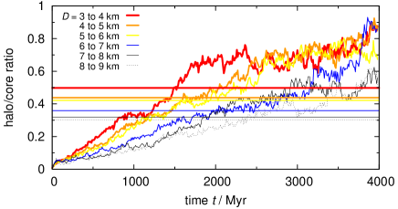
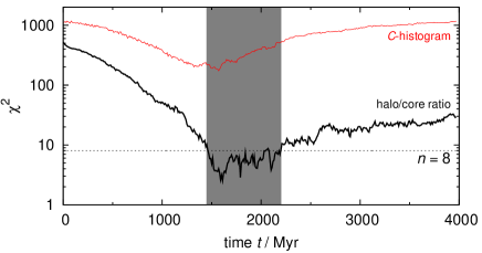
Figure 7: Top panel: the evolution of the halo/core ratio in our simulation for several size bins (colour curves) and its comparison to the observed SDSS ratios in the same bins (horizontal lines). The intersections give age estimates from 1.5 Gyr (for smaller bodies) to 2.2 Gyr (larger bodies). Bottom panel: the corresponding evolution of the $\chi^{2}$ vs time $t$. The dotted line indicates the number $n=8$ of size bins (from $D=2\,{\rm km}$ to $10\,{\rm km}$) in which the $\chi^{2}$ was computed. The best fits (with $\chi^{2}\simeq n$ or smaller) correspond to ages from 1.5 to 2.2 Gyr. For comparison, we also plot a $\chi^{2}(t)$ dependence (red line), computed from the histogram of $C\equiv(a-3.019\,{\rm AU})/10^{H}$ values, which corresponds to the analysis of Vokrouhlický et al. (2006). We use the population of Eos-like asteroids observed by the SDSS in both core and halo for this purpose.

4 Conclusions

Yarkovsky-driven origin seems to be a natural explanation of the halo population. A lucky coincidence that the disruption of the Eos-family parent body occurred close to the moderately strong 9/4 mean motion resonance with Jupiter established a mechanism, in which orbits drifting in semimajor axis due to the Yarkovsky effect are mostly perturbed by this resonance and scattered around in eccentricity and inclination. The total spread of the simulated halo (up to 0.2 in eccentricity, Figure 5), which matches the SDSS observations (Figure 2), also supports our conclusion.

As an important by-product, the process enabled us to independently constrain the age of the family. Moreover, if we analyse the evolution in the proper semimajor axis vs the absolute magnitude $(a_{\rm p},H)$ plane and create a histogram of the quantity $C\equiv(a-3.019\,{\rm AU})/10^{H}$ (i.e. a similar approach as in Vokrouhlický et al. (2006), but now using a full $N$-body model and the SDSS observations for both the core and halo), we can compute an independent $\chi^{2}(t)$ evolution (refer to Figure 7, red line). Since both methods – the halo/core ratios ${\cal R}$ and the $C$-histogram – seem to be reasonable, we can infer the most probable age as an overlap of intervals of low $\chi^{2}(t)$ and this way further decrease its uncertainty, so that $t\simeq 1.5\hbox{ to }1.9\,{\rm Gyr}$.

It is also interesting that the true anomaly at the time of disruption has to be $f\simeq 120^{\circ}\hbox{ to }180^{\circ}$. We performed tests with lower values of $f$ and in these cases the synthetic family has initially a different orientation in the $(a_{\rm p},e_{\rm p})$ plane: the objects are spread from small $a_{\rm p}$ and $e_{\rm p}$ to large $a_{\rm p}$ and $e_{\rm p}$ (cf. Figure 5). Way too many objects thus initially fall in to the $z_{1}$ secular resonance and because such captured orbits cannot drift to small $a_{\rm p}$ and large $e_{\rm p}$ it is then impossible to explain the observed structure of the family and consequently $f\lesssim 120^{\circ}$ is excluded.

Finally, let us emphasize that given the differences between the size-frequency distribution of the halo that of the core, we can exclude a possibility that the Eos halo was created by a purely gravitational process (like the perturbations arising from giant-planet migration).

References

- Brož (2006) Brož, M., 2006. Yarkovsky Effect and the Dynamics of the Solar System. PhD Thesis, Charles Univ.
- Brož et al. (2011) Brož, M., Vokrouhlický, D., Morbidelli, A., Nesvorný, D., Bottke, W. F., Jul. 2011. Did the Hilda collisional family form during the late heavy bombardment? Mon. Not. R. Astron. Soc. 414, 2716–2727.
- Carruba (2009) Carruba, V., May 2009. The (not so) peculiar case of the Padua family. Mon. Not. R. Astron. Soc. 395, 358–377.
- Carruba and Michtchenko (2007) Carruba, V., Michtchenko, T. A., Dec. 2007. A frequency approach to identifying asteroid families. Astron. Astrophys. 475, 1145–1158.
- Cellino et al. (1999) Cellino, A., Michel, P., Tanga, P., Zappalà, V., Paolicchi, P., dell’Oro, A., Sep. 1999. The Velocity-Size Relationship for Members of Asteroid Families and Implications for the Physics of Catastrophic Collisions. Icarus 141, 79–95.
- DeMeo et al. (2009) DeMeo, F. E., Binzel, R. P., Slivan, S. M., Bus, S. J., Jul. 2009. An extension of the Bus asteroid taxonomy into the near-infrared. Icarus 202, 160–180.
- Farinella et al. (1998) Farinella, P., Vokrouhlický, D., Hartmann, W. K., Apr. 1998. Meteorite Delivery via Yarkovsky Orbital Drift. Icarus 132, 378–387.
- Hanuš et al. (2011) Hanuš, J., Ďurech, J., Brož, M., Warner, B. D., Pilcher, F., Stephens, R., Oey, J., Bernasconi, L., Casulli, S., Behrend, R., Polishook, D., Henych, T., Lehký, M., Yoshida, F., Ito, T., Jun. 2011. A study of asteroid pole-latitude distribution based on an extended set of shape models derived by the lightcurve inversion method. Astron. Astrophys. 530, A134.
- Laskar and Robutel (2001) Laskar, J., Robutel, P., Jul. 2001. High order symplectic integrators for perturbed Hamiltonian systems. Celestial Mechanics and Dynamical Astronomy 80, 39–62.
- Levison and Duncan (1994) Levison, H. F., Duncan, M. J., Mar. 1994. The long-term dynamical behavior of short-period comets. Icarus 108, 18–36.
- Masiero et al. (2011) Masiero, J. R., Mainzer, A. K., Grav, T., Bauer, J. M., Cutri, R. M., Dailey, J., Eisenhardt, P. R. M., McMillan, R. S., Spahr, T. B., Skrutskie, M. F., Tholen, D., Walker, R. G., Wright, E. L., DeBaun, E., Elsbury, D., Gautier, IV, T., Gomillion, S., Wilkins, A., Nov. 2011. Main Belt Asteroids with WISE/NEOWISE. I. Preliminary Albedos and Diameters. Astrophys. J. 741, 68.
- Milani and Knezevic (1992) Milani, A., Knezevic, Z., Aug. 1992. Asteroid proper elements and secular resonances. Icarus 98, 211–232.
- Morbidelli et al. (2005) Morbidelli, A., Levison, H. F., Tsiganis, K., Gomes, R., May 2005. Chaotic capture of Jupiter’s Trojan asteroids in the early Solar System. Nature 435, 462–465.
- Parker et al. (2008) Parker, A., Ivezić, Ž., Jurić, M., Lupton, R., Sekora, M. D., Kowalski, A., Nov. 2008. The size distributions of asteroid families in the SDSS Moving Object Catalog 4. Icarus 198, 138–155.
- Čapek and Vokrouhlický (2004) Čapek, D., Vokrouhlický, D., Dec. 2004. The YORP effect with finite thermal conductivity. Icarus 172, 526–536.
- Šidlichovský and Nesvorný (1996) Šidlichovský, M., Nesvorný, D., Mar. 1996. Frequency modified Fourier transform and its applications to asteroids. Celestial Mechanics and Dynamical Astronomy 65, 137–148.
- Vokrouhlický et al. (2006) Vokrouhlický, D., Brož, M., Morbidelli, A., Bottke, W. F., Nesvorný, D., Lazzaro, D., Rivkin, A. S., May 2006. Yarkovsky footprints in the Eos family. Icarus 182, 92–117.
- Zappalà et al. (2000) Zappalà, V., Bendjoya, P., Cellino, A., Di Martino, M., Doressoundiram, A., Manara, A., Migliorini, F., May 2000. Fugitives from the Eos Family: First Spectroscopic Confirmation. Icarus 145, 4–11.
- Zappalà et al. (1995) Zappalà, V., Bendjoya, P., Cellino, A., Farinella, P., Froeschlè, C., Aug. 1995. Asteroid families: Search of a 12,487-asteroid sample using two different clustering techniques. Icarus 116, 291–314.