Stochastically-induced bistability in chemical reaction systems

Abstract

We study a stochastic two-species chemical reaction system with two mechanisms. One mechanism consists of chemical interactions which govern the overall drift of species amounts in the system; the other mechanism consists of resampling, branching or splitting which makes unbiased perturbative changes to species amounts. Our results show that in a system with a large but bounded capacity, certain combinations of these two types of interactions can lead to stochastically-induced bistability. Depending on the relative magnitudes of the rates of these two sets of interactions, bistability can occur in two distinct ways with different dynamical signatures.

T1Supported by the New Researchers Grant (F00637-126232) from FQRNT (Fonds de recherche du Québec Nature et technologies).

and

1 Introduction

Recent advances in measurement technology have enabled scientists to observe molecular dynamics in single cells and to study the cell-to-cell variability (Brehm-Stecher and Johnson B-S ). Many studies have shown that variability observed in genetically identical cells is due to noise that is inherent to biochemical reactions happening within each cell (McAdams and Arkin MA , Elowitz et al. El ). Understanding how intracellular mechanisms are affected by this intrinsic noise is an important challenge for systems biology. Determining what role this noise plays in creating phenotypic heterogeneity has many practical consequences (Avery Av ).

An important feature in cellular dynamics is bistability, the alternation between two different stable states for a molecular species. This feature is present in many gene-expression systems, where a gene alternates between two types of states (“on” and “off”) regulating the production of a protein. It is also present in many phosphorylation switches in signaling pathways. Causes for bistable behavior can be deterministic, but many bistable switching patterns are enabled by stochastic fluctuations. It is often assumed that it follows from the existence of two stable equilibria in the deterministic drift and the ability of infrequent large fluctuations to pull the system from a basin of attraction of one equilibirum to the other. There are also cases of chemical dynamics in which bistability is not possible in the deterministic model, but is possible in the stochastic model of the same chemical reaction system (Samoilov et al. SPA , Bishop and Qian BQ ). Metastable behavior is also sometimes observed (Robert et al. LydR ).

In addition to noise inherent to biochemical reactions, cells also experience fluctuations in molecular composition due to cell division. This source of noise is significant, and also difficult to separate from the noise due to biochemical reactions (Huh and Paulsson Pa1 , Pa2 ). In this paper we investigate under what conditions a system of chemical reactions in a cell can use these two sources of noise to exhibit bistable or metastable behavior in their molecular composition.

We would like to emphasize a couple of points observed in the literature. First, the rate of switching between two states is important for cellular development and survival (Acar et al. vO ). Time-scales on which transitions between stable states happen varies whole orders of magnitude over different systems. For example, in the lysogenic state of E. coli the time-scale of switching between states is slow (Zong et al. ZSSSG )—once per $10^{8}$ cell generations—as determined from the activity of a controlling protein. In the case of gene expression in S. cerevisiae the switching time-scale is fast (Kaufmann et al. KYMvO )—once per $8.33$ generations—and switching times between mother and daughter cells are correlated in a way that takes several generations to dissipate. Second, both the strength and the distribution of noise affects whether bistability will occur and what the final outcomes will be. Samoilov et al. SPA and Bishop and Qian BQ show that auxiliary chemical reactions can induce a dynamic switching behavior in the enzymatic PdP cycle, and that final dynamics is determined by the noise of the additional reactions. In the bistable switch of lactose operon of E. coli Robert et al. LydR show that both cellular growth rate and the molecular concentration levels influence the ability to switch. Huh and Paulsson Pa2 showed that the type of the cellular division mechanism also plays an important role in the form of the final dynamics. We interpret these observations vis-a-vis our results in the Discussion section.

Finally, we note that bistablility in a stochastic population system is not limited to chemical dynamics. In a genetic population, mutation and selection may lead to alternating fixation in one of two genotypes. In an ecological population, interactions between species can lead to dynamics where two competing species are switching for dominance. We note that our analysis and results apply to any population model described by a density dependent Markov jump process.

1.1 Outline of results

We examine qualitatively different ways in which switching between stable states is a result of a stochastic effect in a population modeled by density dependent Markov jump processes. In addition to noise inherent to the reaction system, we include an intrinsically noisy splitting/resampling mechanism in the system. In many stochastic branching models an entity will (upon reproduction, division, duplication, etc.) produce offspring identical to itself. Here we model the division as unbiased but variable. When a cell divides its molecules are randomly allocated to its daughter cells, only on average replicating the parent’s molecular composition. We will show that introducing such a splitting process at a sufficiently high rate can produce switching dynamics in which previously unattainable states become attainable. We will exploit the fact that these two sets of mechanisms (reactions in the system and changes due to unbiased resampling/splitting of the system) may operate on different time-scales.

We consider the following question: which qualitatively different types of behavior can we observe and under which time scaling regimes? The short answer is as follows: (1) If the resampling mechanism is “slower” than the reaction dynamics, then the system behavior will entirely depend on the nonlinear dynamics of the reactions: in case the underlying deterministic system has multiple stable equilibria, the stochastic process will behave as a Markov chain switching between these states. (2) If the resampling mechanism is much “faster” than the reaction dynamics, then the system behavior will not depend on the details of the reaction dynamics, and will behave as a Markov chain switching between two extremes (zero and capacity) of the system. We define a single parameter based on the rates of the two mechanisms that makes the meaning of “faster” and “slower” in the statements above mathematically precise.

We show that a fast but unbiased resampling mechanism may be necessary to produce bistable behavior that the reaction dynamics cannot exhibit. We further show that the two cases, (1) and (2), produce qualitatively different dynamical signatures, in terms of switching times and stable points. Since our analysis only depends on general features (unbiasedness and time-scale of the rate) of the resampling mechanism, one can also use a set of auxiliary reactions instead of resampling. There are other types of noisy mechanisms that one could consider; however, our goal is to stress that adding noise with even small changes (relative to the size of the system) can produce bistable behavior. The additional noise achieves this either by: (1) introducing small perturbations to a dynamical system that already has the required properties for bistability or (2) occurring so frequently that the details of the dynamical system are irrelevant and the system is pushed to its extreme (zero or capacity) amounts.

2 Description of the process

2.1 Stochastic model for reaction dynamics

In the customary notation for interaction of chemical species labeled $A,B,\ldots,$

$$\bigl{\{}a_{i}A+b_{i}B+\cdots\longrightarrow a_{i}^{\prime}A+b_{i}^{\prime}B+\cdots\bigr{\}}_{i=1,\ldots,k}$$ (1)

denotes a system of reactions indexed by $i=1,\ldots,k$ in which $a_{i},b_{i},\ldots\in\mathbb{Z}^{+}$ molecules of types $A,B,\ldots$ respectively react and produce $a_{i}^{\prime},b_{i}^{\prime},\ldots\in\mathbb{Z}^{+}$ molecules of these types. Each reaction $i$ has a reaction rate $\lambda_{i}$, a time and state-dependent rate of occurrences of this reaction. If $X_{A}(t),X_{B}(t),\ldots$ denote the number of molecules of type $A,B,\ldots$ respectively at time $t\geq 0$, then $X(t)=(X_{A}(t),X_{B}(t),\ldots)$ evolves as a Markov Jump Process with jump sizes $\{(a_{i}^{\prime}-a_{i},b_{i}^{\prime}-b_{i},\ldots)\}$ occurring at rates $\lambda_{i}(X_{A}(t),X_{B}(t),\ldots)$.

The reaction formalism (1) can also be used to describe other systems of interacting entities under a well-mixed spatial assumption. For example, evolution of an SIS epidemic is expressed as $I+S\to 2I$ (infection), $I\to S$ (recovery); a two-allele Moran model with mutation from population genetics can be expressed as $A\to B,B\to A$ (mutation), $A+B\to 2A,A+B\to 2B$ (resampling).

For simplicity, we consider the effect of a system of chemical reactions on essentially a single molecular species $A$. We include the effect of only one other species $B$ which satisfies a conservation relation with $A$. This means that every reaction involving $A$ and $B$ is of the form $aA+bB\to(a+\zeta)A+(b-\zeta)B$ for some $\zeta\in\{-a,\ldots,b\}$, and it ensures that the state space of our system is one-dimensional determined by $(X_{A}(t),t\geq 0)$. The rationale for such a conservation law could come from a cellular environment which is limited (by a factor such as space, or availability of nutrients or catalysts), or a molecular species whose type can take two different forms (e.g., a gene that has two allelic types).

We also assume the following properties for the reaction dynamics: [(4)]

The amount of species $X_{A}(t)$ is bounded above by the system capacity $N$ and below by $0$. The rate of any reaction that decreases the amount of $A$ is zero when $X_{A}=0$, and the rate of any reaction that increases the amount of $A$ is zero when $X_{A}=N$.

The drift at $0$ and $N$ of the overall reaction dynamics is directed toward the interior

$$\frac{d}{ds}\mathbf{E}\bigl{[}X_{A}(s)|X_{A}(t)=0\bigr{]}|_{s=t}>0,\qquad\frac{d}{ds}\mathbf{E}\bigl{[}X_{A}(s)|X_{A}(t)=N\bigr{]}|_{s=t}<0.$$

The form of reaction rates $\lambda$ is governed by the law of (stochastic) mass-action kinetics. A reaction of the form

$$aA+bB\stackrel{{\scriptstyle\kappa}}{{\to}}a^{\prime}A+b^{\prime}B$$

has rate $\lambda(X(t))=\kappa(X_{A}(t))_{a}(X_{B}(t))_{b}=\kappa(X_{A}(t))_{a}(N-X_{A}(t))_{b}$. Here $(Z)_{c}$ denotes the falling factorial $(Z)_{c}=Z(Z-1)\cdots(Z-c+1)$. When we renormalize $X_{A}(t)$ by its maximum value $N$, we will also need the “scaled falling factorial” $(z)_{c,N}$ defined by

$$(z)_{c,N}:=N^{-c}(Nz)_{c}=z\biggl{(}z-\frac{1}{N}\biggr{)}\biggl{(}z-\frac{2}{N}\biggr{)}\cdots\biggl{(}z-\frac{c-1}{N}\biggr{)},$$

(2)

$$\eqntext{0\leq z\leq 1.}$$ (3)

Note that $\lim_{N\to\infty}(z)_{c,N}=z^{c}$ for fixed $z$ and $c$. The constant $\kappa>0$ is independent of the state $(X_{A}(t),X_{B}(t)=N-X_{A}(t))$ but will depend on the scaling parameter $N$, $\kappa=\kappa(N)$. We do not necessarily assume that $\kappa(N)$ has the “standard” scaling form $\kappa(N)=\tilde{\kappa}N^{1-(a+b)}$.

The effect on $A$ from any other species in the system is subsumed into the values of the rate constants $\kappa$, and are assumed to be state-independent.

Assumption (1) ensures that $X_{A}(\cdot)\in\{0,\ldots,N\}$ where $N$ serves as the system-size parameter, while assumption (2) ensures the reaction system does not get absorbed at either boundary $\{0,N\}$. Assumption (3) is not essential, but with an explicit scaling of the rate $\kappa(N)$ in terms of $N$, the polynomial form of the rates $\lambda$ will make it easy to also establish the scaling of the rates $\lambda(X(t))$ in terms of $N$ under a rescaling of the species amounts $X_{A}$ [we will occasionally use the notation $\kappa(N)$ for $\kappa$ when awareness of dependence on $N$ is key]. Assumption (4) is made to absorb the effect of the environment and other species, the changes of which we will not keep track of explicitly.

Under these assumptions, our reaction network system can now be expressed by

$$\bigl{\{}aA+bB\mathop{\longrightarrow}^{\kappa_{\zeta}^{ab}}(a+\zeta)A+(b-\zeta)B\bigr{\}}_{a\in\{0,\ldots,N\},b\in\{0,\ldots,N\},\zeta\in\{-a,\ldots,b\}}$$ (4)

with reaction rates of the form $\lambda_{\zeta}^{ab}(x)=\kappa_{\zeta}^{ab}\cdot(x)_{a}(N-x)_{b}$.

Since the dynamics of the system depends on its overall drift, it will be useful to distinguish a subset of reactions whose combined effect on $\mathbf{E}[X_{A}(t)]$ is zero, irrespective of the value of $X_{A}(t)$. In other words, we will group reactions into a subset which contributes zero to the drift (“balanced”), and the rest which are responsible for all of the drift (“biased”). Note that the definition of balance below is made for subsets of reactions—one cannot determine for a single reaction on its own whether it is balanced or not—in order for a reaction to be balanced it needs to belong to a balanced subset.

Let $\mathcal{I}$ denote the set of all triples $(a,b,\zeta)$ for which a reaction as written in (4) is present in the system. A subset of reactions is defined as “balanced” $\mathcal{I}^{\operatorname{bal}}\subset\mathcal{I}$ if for some fixed reactant amounts $a,b$, it satisfies

$$\sum_{\zeta:(a,b,\zeta)\in\mathcal{I}^{\operatorname{bal}}}\zeta\lambda_{\zeta}^{ab}(x)=0\qquad\forall x\quad\Longleftrightarrow\quad\sum_{\zeta\dvtx(a,b,\zeta)\in\mathcal{I}^{\operatorname{bal}}}\zeta\kappa_{\zeta}^{ab}=0.$$

A reaction $(a,b,\zeta)\in\mathcal{I}$ that is part of some balanced subset is called “balanced” and all the remaining reactions that are not part of any balanced subset are called “biased,” $\mathcal{I}^{\operatorname{bia}}=\mathcal{I}-\mathcal{I}^{\operatorname{bal}}$. Note that our notion of balance is very restrictive and is not related to standard notions of chemical reactions.

For any balanced reaction $(a,b,\zeta)\in\mathcal{I}^{\operatorname{bal}}$, there is necessarily a reaction $(a,b,\zeta^{\prime})\in\mathcal{I}^{\operatorname{bal}}$ with $\zeta,\zeta^{\prime}$ having opposite signs (though not necessarily of the same size). Hence, a reaction $(a,b,\zeta)\in\mathcal{I}^{\operatorname{bal}}$ cannot have nontrivial rate at the boundaries of the system: if $\lambda_{\zeta}^{a,b}(0)>0$ for some $\zeta>0$, then the balance condition would imply the existence of some $\zeta^{\prime}<0$ for which $\lambda_{\zeta^{\prime}}^{a,b}(0)>0$, which would violate assumption (1) by allowing $X_{A}$ to drop below $0$ upon a single further $(a,b,\zeta^{\prime})$ reaction. Consequently, the boundaries $0$ and $N$ are absorbing for the balanced subsystem of reactions, and for all $(a,b,\zeta^{\prime})\in\mathcal{I}^{\operatorname{bal}}$ we must have both $a>0$ and $b>0$. Since assumption (2) does not allow the boundary $\{0,N\}$ to be absorbing for the full dynamics, this further implies that there is at least one biased reaction $(a,b,\zeta)\in\mathcal{I}^{\operatorname{bia}}$ with $\zeta>0$ and $\zeta\lambda_{\zeta}^{ab}(0)>0$, hence $a=0,b>0$; and there is at least one biased reaction $(a,b,\zeta^{\prime})\in\mathcal{I}^{\operatorname{bia}}$ with $\zeta^{\prime}<0$, and $\zeta^{\prime}\lambda_{\zeta^{\prime}}^{a,0}(N)<0$, hence $a>0,b=0$.

The continuous-time Markov jump process model for the reaction dynamics can be expressed in terms of a set of Poisson processes under a random time change. Given a collection $\{Y_{\zeta}^{ab}\}_{(a,b,\zeta)\in\mathcal{I}}$ of independent unit-rate Poisson processes, the state of the system can be expressed as a solution to the stochastic equation (see KuAPP or BKPR for details)

$$X_{A}(t) = X_{A}(0)+\sum_{(a,b,\zeta)\in\mathcal{I}}\zeta Y_{\zeta}^{ab}\biggl{(}\int_{0}^{t}\lambda_{\zeta}^{ab}\bigl{(}X_{A}(s)\bigr{)}\,ds\biggr{)}$$

$$= X_{A}(0)+\sum_{(a,b,\zeta)\in\mathcal{I}}\zeta\hat{Y}_{\zeta}^{ab}\biggl{(}\int_{0}^{t}\lambda_{\zeta}^{ab}\bigl{(}X_{A}(s)\bigr{)}\,ds\biggr{)}+\int_{0}^{t}F\bigl{(}X_{A}(s)\bigr{)}\,ds,$$

where $\{\hat{Y}_{\zeta}^{ab}\}_{(a,b,\zeta)\in\mathcal{I}}$ are centered Poisson processes $\hat{Y}(\lambda t):=Y(\lambda t)-\lambda t$, and

$$F(x)=\sum_{(a,b,\zeta)\in\mathcal{I}}\zeta\lambda_{\zeta}^{ab}(x)=\sum_{(a,b,\zeta)\in\mathcal{I}^{\operatorname{bia}}}\zeta\kappa_{\zeta}^{ab}(x)_{a}(N-x)_{b}.$$

Since the capacity $N$ of the system may be arbitrarily large, we will consider a “standard” rescaling of the system; see, for example, EK , Chapter 11.2. Let $X_{N}(t)=N^{-1}X_{A}(t)$, then

$$X_{N}(t) = X_{N}(0)$$

$${}+\sum_{(\zeta,a,b)\in\mathcal{I}}N^{-1}\zeta\hat{Y}_{\zeta}^{ab}\biggl{(}N^{a+b}\kappa_{\zeta}^{ab}\int_{0}^{t}\bigl{(}X_{N}(s)\bigr{)}_{a,N}\bigl{(}1-X_{N}(s)\bigr{)}_{b,N}\,ds\biggr{)}$$

$${}+\int_{0}^{t}F_{N}\bigl{(}X_{N}(s)\bigr{)}\,ds,$$

where the local drift of the renormalized system is given by

$$F_{N}(x)=\sum_{(\zeta,a,b)\in\mathcal{I}^{\operatorname{bia}}}N^{a+b-1}\zeta\kappa_{\zeta}^{ab}(x)_{a,N}(1-x)_{b,N}.$$

The most important feature of the Markov jump process model is the relationship of the variance to the drift. Note that we can write (2.1) as

$$X_{N}(t)=X_{N}(0)+M_{N}(t)+\int_{0}^{t}F_{N}\bigl{(}X_{N}(s)\bigr{)}\,ds,$$

where the second term from (2.1), a weighted sum of time-changed centered Poisson processes, is a martingale $M_{N}(t)$ whose quadratic variation satisfies

$$[M_{N}]_{t}=\sum_{(\zeta,a,b)\in\mathcal{I}}N^{-2}\zeta^{2}Y_{\zeta}^{ab}\biggl{(}N^{a+b}\kappa_{\zeta}^{ab}\int_{0}^{t}\bigl{(}X_{N}(s)\bigr{)}_{a,N}\bigl{(}1-X_{N}(s)\bigr{)}_{b,N}\,ds\biggr{)}.$$

Hence, if $\mathcal{F}_{t}=\sigma(X(s),0\leq s\leq t)$ denotes the natural filtration of the process, then

$$\frac{d}{ds}\mathbf{E}\bigl{[}X_{N}(s)|\mathcal{F}_{t}\bigr{]}|_{s=t}$$

$$\qquad=\mathbf{E}\bigl{[}F_{N}\bigl{(}X_{N}(t)\bigr{)}|\mathcal{F}_{t}\bigr{]}$$

$$\qquad=\sum_{(\zeta,a,b)\in\mathcal{I}^{\operatorname{bia}}}N^{a+b-1}\zeta\kappa_{\zeta}^{ab}\bigl{(}X_{N}(t)\bigr{)}_{a,N}\bigl{(}1-X_{N}(t)\bigr{)}_{b,N},$$

$$\frac{d}{ds}\mathbf{E}\bigl{[}\bigl{(}X_{N}(s)-\mathbf{E}\bigl{[}X_{N}(s)\bigr{]}\bigr{)}^{2}|\mathcal{F}_{t}\bigr{]}|_{s=t}$$

$$\qquad=\frac{d}{ds}\mathbf{E}\bigl{[}[M_{N}]_{s}|\mathcal{F}_{t}\bigr{]}|_{s=t}$$

$$\qquad=\sum_{(\zeta,a,b)\in\mathcal{I}^{\operatorname{bal}}\cup\mathcal{I}^{\operatorname{bia}}}N^{a+b-2}\zeta^{2}\kappa_{\zeta}^{ab}\bigl{(}X_{N}(t)\bigr{)}_{a,N}\bigl{(}1-X_{N}(t)\bigr{)}_{b,N}.$$

Recall that the reaction rates $\kappa^{ab}_{\zeta}=\kappa^{ab}_{\zeta}(N)$ also depend on the scaling parameter $N$. The standard scaling for a reaction constant is $\kappa^{ab}_{\zeta}(N)=\tilde{\kappa}^{ab}_{\zeta}N^{1-(a+b)}$ for some $N$-independent constant $\tilde{\kappa}^{ab}_{\zeta}$. However, regardless of the chosen scaling of $\kappa^{ab}_{\zeta}$, for biased reactions $\mathcal{I}^{\operatorname{bia}}$ the order of magnitude for each summand in the infinitesimal variance $\frac{d}{ds}\mathbf{E}[[M_{N}]_{s}|\mathcal{F}_{t}]|_{s=t}$ is $N^{-1}$ times smaller than the corresponding summand in the infinitesimal drift $\mathbf{E}[F_{N}(X_{N}(s))|\mathcal{F}_{t}]|_{s=t}$. This constrains the possible limiting dynamics of $X_{N}$. Suppose the scaling of the rates is $\kappa^{ab}_{\zeta}=N^{1-(a+b)}\tilde{\kappa}^{ab}_{\zeta}$, and note that then $F_{N}(x)\to\sum_{(\zeta,a,b)\in\mathcal{I}^{\operatorname{bia}}}\zeta\tilde{\kappa}_{\zeta}^{ab}x^{a}(1-x)^{b}$ uniformly for $x\in[0,1]$. As established in Ku77 , in the limit as $N\to\infty$ the drift overpowers the noise and, provided $X_{N}(0)\Rightarrow x(0)$, the renormalized process $(X_{N}(t),t\geq 0)$ converges in distribution (in the Skorokhod topology of cadlag paths) to a solution $(x(t),t\geq 0)$ of the ordinary differential equation

$$x(t)=x(0)+\int_{0}^{t}\sum_{(\zeta,a,b)\in\mathcal{I}^{\operatorname{bia}}}\zeta\tilde{\kappa}_{\zeta}^{ab}x(s)^{a}\bigl{(}1-x(s)\bigr{)}^{b}\,ds.$$ (6)

In fact, if the scaling of the reaction constants $\kappa^{ab}_{\zeta}$ is not standard, but is consistent for both balanced and biased reactions in terms of the polynomial order of the rate function $\lambda^{ab}_{\zeta}$, then the same deterministic limit is obtained under an appropriate time rescaling.

The only way to get a stochastic limiting object for $X_{N}$ is for at least one subset of balanced reactions to have a rate constant with a different scaling in $N$. This different scaling needs to be such that the noise term due to this subset of reactions will be of the same order of magnitude as the overall drift from the biased reactions. This would require a specific separation of time-scales for balanced versus biased reactions. Although we do not exclude this possibility from our analysis (see definition of $\varepsilon_{A}$ at the end of this section), our emphasis in this paper is on separating the time-scales in terms of contribution of an additional source of noise, and its ability to produce nontrivial random limiting objects for $X_{N}$.

2.2 Stochastic model for resampling, branching or splitting

We now introduce the additional mechanism in the system that describes changes to species amounts due to the effect of splitting, branching or resampling, which also effects the species count. For intracellular molecular populations, our first model of splitting was motivated by a simple double-then-divide principle: the cell will first double in size by replicating its constituent molecular species, and then allocate approximately one half of this doubled material into each daughter cell—the allocation mechanism is not perfect and will make random error from the original (undoubled) amount. For genetic populations, common models for resampling follow the Wright–Fisher or the Moran neutral reproduction law: each individual of the offspring population chooses at random from the diploid version of the current population’s genes what to inherit—the resampling mechanism is such that an allele of one type in one generation may at random be replaced in the subsequent generation by an allele of the other type. These two are both examples of a general mechanism with the following key properties that we assume for splitting/resampling: [(5)]

The splitting/resampling occurs at rate $\gamma(x,N)$ that depends on: the current state $X_{A}=x$ of the system and the scaling parameter $N$; conditional on $X_{A}=x$ it is independent of reactions.

The change in the species amount $X_{A}$ due to a splitting/resampling event has the distribution $p_{x,y}=\mathbf{P}[X_{A}(t)=y|X_{A}(t-)=x]$ that have absorbing boundaries $p_{0,0}=1,p_{N,N}=1$, and that are unbiased

$$\mu_{N}(x)=\sum_{y}yp_{x,y}=x\qquad\forall x\in\{0,1,\ldots,N\}.$$

We also assume, for some of our results, that the rate $\gamma(x,N)$ and distribution $\{p_{x,y}\}$ are such that:

1. [(${7}^{*}$)]

2. The change sizes are asymptotically uniformly bounded,

   1. [($7^{*}.\mathrm{a}$)]

   2. $\displaystyle\forall\Delta>0\qquad\sup_{x}\gamma(x,N)\sum_{y:N^{-1}|y-x|\geq\Delta}p_{x,y}\to 0\qquad\mbox{as }N\to\infty,$

   and the change size variance $\sigma^{2}_{N}(x)=\sum_{y}(y-x)^{2}p_{x,y}$ is asymptotically given by

   1. [($7^{*}.\mathrm{b}$)]

   2. $\displaystyle\sup_{x}\bigl{|}\gamma(x,N)N^{-2}\sigma^{2}_{N}(x)-\tilde{\gamma}^{2}\tilde{\sigma}^{2}\bigl{(}N^{-1}x\bigr{)}\bigr{|}\to 0\qquad\mbox{as }N\to\infty$

   for some constant $\tilde{\gamma}>0$ and function $\tilde{\sigma}(\cdot)$ that are independent of $N$, and such that $x\mapsto\tilde{\sigma}^{2}(x)$ is continuous with $\tilde{\sigma}^{2}(x)>0,\forall x\in(0,1)$ and $\tilde{\sigma}^{2}(0)=\tilde{\sigma}^{2}(1)=0$.

Unbiasedness in assumption (6) could be replaced by an “asymptotic unbiasedness” assumption $N^{-1}|\mu_{N}(x)-x|\to 0\mbox{ as }N\to\infty$, but for the sake of simplicity we assume $\mu_{N}(x)=x$. Absorption in assumption (6) implies splitting is noiseless on the boundaries regardless of its time-scale. When the additional assumption (${7}^{*}$) holds (as we will assume for our results in Section 2.3), the splitting mechanism contributes diffusively to the limit of the renormalized species count $X_{N}$. However, we will also examine the case when the rate of the splitting mechanism is on a slower time-scale (in Section 3.1), as well as the case when it is on a faster time-scale (in Section 4.1). The condition that $\tilde{\sigma}^{2}$ has boundary values $\tilde{\sigma}^{2}(0)=\tilde{\sigma}^{2}(1)=0$ is natural given that any splitting or resampling mechanism should absorb at the boundaries as indicated by $p_{0,0}=p_{N,N}=1$.

[(HG)] One example of a splitting mechanism would be to completely randomly reallocate the doubled content of a parent cell into daughter cells. If the initial content is $(X_{A},X_{B})=(x,N-x)$, and the doubled content $(2x,2(N-x))$ is partitioned in a single swoop (draw without replacement) into two sets of $N$ molecules (one for each daughter cell), then the content in each daughter cell has the hypergeometric distribution (below we keep track of an arbitrarily chosen single lineage)

$$p_{x,y}=\mathbf{P}\bigl{[}X_{A}(t)=y|X_{A}(t-)=x\bigr{]}=\frac{{2x\choose y}{2N-2x\choose N-y}}{{2N\choose N}},$$

$$\eqntext{0\lor(2x-N)\leq y\leq 2x\land N.}$$ (7)

The change in the species count is clearly unbiased $\mu_{N}(x)=\sum_{y=0\lor N-2x}^{2x\land N}yp_{x,y}=x$, with variance

$$\sigma^{2}_{N}(x)=\sum_{y=0\lor N-2x}^{2x\land N}(y-x)^{2}p_{x,y}=\frac{N2x(2N-2x)}{4N^{2}}\biggl{(}1-\frac{N-1}{2N-1}\biggr{)}=\frac{x(N-x)}{2N-1}.$$

Then assumption (${7}^{*}$) will hold if $\gamma(x,N)=\tilde{\gamma}^{2}N$ and $\tilde{\sigma}^{2}(x)=\frac{1}{2}x(1-x)$, since for (${7}^{*}$.a) we have

$$\sup_{x}\bigl{|}\gamma(x,N)N^{-2}\sigma^{2}_{N}(x)-\tilde{\gamma}^{2}\tilde{\sigma}^{2}\bigl{(}N^{-1}x\bigr{)}\bigr{|} = \tilde{\gamma}^{2}\sup_{x}\biggl{|}\frac{x(N-x)}{N(2N-1)}-\frac{1}{2}\frac{x}{N}\biggl{(}1-\frac{x}{N}\biggr{)}\biggr{|}$$

$$\to 0$$

and using tail bounds for the hypergeometric distribution Ch $\sum_{y=x+N\Delta}^{N}p_{x,y}\leq e^{-2\Delta^{2}N}$ independently of $x$, and for (${7}^{*}$.b) we have

$$\gamma(x,N)\sup_{x}\sum_{y:|y-x|\geq N\Delta}p_{x,y}\leq 2\tilde{\gamma}^{2}Ne^{-2\Delta^{2}N}\to 0.$$

[(Bin)] Another example would be to sample with replacement from the population in which each offspring picks its type randomly from any individual in the parent generation. If the initial count is $X_{A}=x$, then the count in the next generation has the binomial distribution

$$p_{x,y}=\mathbf{P}\bigl{[}X_{A}(t)=y|X_{A}(t-)=x\bigr{]}={\pmatrix{N\cr y}}\biggl{(}\frac{x}{N}\biggr{)}^{y}\biggl{(}1-\frac{x}{N}\biggr{)}^{N-y},\qquad 0\leq y\leq N.$$

This form of resampling is used in (the haploid version of) the Wright–Fisher model for genetic drift (e.g., DurDNA Section 1.2). It is also used as the prototype of a splitting mechanism of simple “independent segregation” of division of cells Pa2 . This distribution is again unbiased, and assumption (${7}^{*}$) will hold if $\gamma(x,N)=\frac{1}{2}\tilde{\gamma}^{2}N$ for some constant $\tilde{\gamma}^{2}>0$. Using similar arguments as above, it is then easy to show that both (${7}^{*}$.a) and (${7}^{*}$.b) will hold with $\tilde{\sigma}^{2}(x)=\frac{1}{2}x(1-x)$.

[(Bern)] Finally, the simplest example of a splitting/resampling mechanism is to have a single amount error in the daughter cell (or the next generation), and to have the rate at which the error occurs be proportional to both the current amount $X_{A}=x$ and the amount of $X_{B}=N-x$. Errors from imperfect division will result in $\pm$ change with equal probability

$$p_{x,x-1}=p_{x,x+1}=1/2.$$

This distribution is clearly unbiased, and assumption (${7}^{*}$) will hold if the rate of error occurrences is $\gamma(x,N)=\frac{1}{2}\tilde{\gamma}^{2}N^{2}\frac{x}{N}(1-\frac{x}{N})$ for some $\tilde{\gamma}^{2}>0$, with the limiting variance $\tilde{\sigma}^{2}(x)=\frac{1}{2}x(1-x)$.
This form of resampling is used in the Moran model for genetic drift (e.g., DurDNA Section 1.5). It is also used in Pa2 as an example of an “ordered segregation” splitting mechanism for cell division (self volume exclusion partitioning error, Pa2 Supporting Information). In a cellular system it could also be described as a set of balanced reactions $A+B\to 2A,A+B\to 2B$ with mass-action dynamics and appropriately scaled rate constants.

We note that, from the perspective of limiting results, the differences in the specific details of the mechanism will not be important. The only feature of relevance will be the order of magnitude of the prelimiting rate $\gamma(x,N)$ and the form of the limiting variance $\tilde{\sigma}^{2}(x)$. There are many other types of splitting, branching or resampling mechanisms, yielding a different form for the limiting variance. They are easy to construct in case of small changes that result in single count errors, via a range of birth–death probability distributions. We shall see, in both Section 3 and Section 4, how the actual form for the variance $\tilde{\sigma}^{2}(x)$ affects the qualitative behavior of the limit of the renormalized process.

The changes due to this additional mechanism can also be expressed in terms of a Poisson processes under a random time change. Let $Y_{\gamma}$ be a counting process with state-dependent rate $\gamma(x,N)$, and $\{Z(x,s)\}_{0\leq x\leq N}$ be independent random variables with probability distribution $p_{x,\cdot}$ for any $s\geq 0$. A change due to splitting or resampling can be represented as a stochastic integral $\int_{0}^{t}(Z(X(s-),s)-X(s-))\,dY_{\gamma}(s)$. The evolution in species count due to both reaction dynamics and splitting is

$$X_{A}(t) = X_{A}(0)+\sum_{(\zeta,a,b)\in I}\zeta\hat{Y}_{\zeta}^{ab}\biggl{(}\int_{0}^{t}\lambda_{\zeta}^{ab}\bigl{(}X_{A}(s)\bigr{)}\,ds\biggr{)}+\int_{0}^{t}F\bigl{(}X_{A}(s)\bigr{)}\,ds$$

$${}+\int_{0}^{t}\bigl{(}Z\bigl{(}X_{A}(s-),s\bigr{)}-X_{A}(s-)\bigr{)}\,dY_{\gamma}(s);$$

hence for the rescaled system $X_{N}=N^{-1}X_{A}$ we have

$$X_{N}(t) = X_{N}(0)$$

$${}+N^{-1}\sum_{(\zeta,a,b)\in\mathcal{I}}\zeta\hat{Y}_{\zeta}^{ab}\biggl{(}N^{a+b}\kappa_{\zeta}^{ab}\int_{0}^{t}\bigl{(}X_{N}(s)\bigr{)}_{a,N}\bigl{(}1-X_{N}(s)\bigr{)}_{b,N}\,ds\biggr{)}$$

$${}+\int_{0}^{t}F_{N}\bigl{(}X(s)\bigr{)}\,ds$$

$${}+\int_{0}^{t}\bigl{(}N^{-1}Z\bigl{(}NX_{N}(s-),s\bigr{)}-X_{N}(s-)\bigr{)}\,d\hat{Y}_{\gamma}(s)$$

$${}+\int_{0}^{t}\bigl{(}N^{-1}Z\bigl{(}NX_{N}(s-),s\bigr{)}-X_{N}(s-)\bigr{)}\gamma\bigl{(}NX_{N}(s),N\bigr{)}\,ds$$

$$= X_{N}(0)+M_{N,\gamma}(t)+\int_{0}^{t}F_{N}\bigl{(}X(s)\bigr{)}\,ds$$

$${}+\int_{0}^{t}N^{-1}\bigl{(}Z\bigl{(}NX_{N}(s-),s\bigr{)}-NX_{N}(s-)\bigr{)}\gamma\bigl{(}NX_{N}(s),N\bigr{)}\,ds.$$

We still have

$$F_{N}(x)=\sum_{(\zeta,a,b)\in\mathcal{I}^{\operatorname{bia}}}N^{a+b-1}\zeta\kappa_{\zeta}^{ab}(N)(x)_{a,N}(1-x)_{b,N},$$ (7)

but now $M_{N,\gamma}$ denotes the martingale formed by the second and fourth summand in (2.2) whose quadratic variation is

$$[M_{N,\gamma}]_{t}$$

$$\qquad=\sum_{(\zeta,a,b)\in\mathcal{I}}N^{-2}\zeta^{2}Y_{\zeta}^{ab}\biggl{(}N^{a+b}\kappa_{\zeta}^{ab}(N)\int_{0}^{t}\bigl{(}X_{N}(s)\bigr{)}_{a,N}\bigl{(}1-X_{N}(s)\bigr{)}_{b,N}\,ds\biggr{)}$$ (8)

$$\qquad\quad{}+\int_{0}^{t}N^{-2}\bigl{(}Z\bigl{(}NX_{N}(s-),s\bigr{)}-NX_{N}(s-)\bigr{)}^{2}\,dY_{\gamma}(s).$$

Note that since the two mechanisms are driven by independent Poisson processes, there is no quadratic covariation contribution. Since $\mathbf{E}_{p_{x,\cdot}}[Z(x,s)-x]=0$ for all $s\geq 0$ and $x\in\{0,\ldots,N\}$, the infinitesimal mean still satisfies

$$\frac{d}{ds}\mathbf{E}\bigl{[}X_{N}(s)|\mathcal{F}_{t}\bigr{]}\Big{|}_{s=t}$$

$$\qquad=\mathbf{E}\bigl{[}F_{N}\bigl{(}X_{N}(t)\bigr{)}|\mathcal{F}_{t}\bigr{]}$$ (9)

$$\qquad=\sum_{(\zeta,a,b)\in\mathcal{I}^{\operatorname{bia}}}N^{a+b-1}\zeta\kappa_{\zeta}^{ab}(N)\bigl{(}X_{N}(t)\bigr{)}_{a,N}\bigl{(}1-X_{N}(t)\bigr{)}_{b,N};$$

on the other hand, the infinitesimal variance now satisfies

$$\frac{d}{ds}\mathbf{E}\bigl{[}\bigl{(}X_{N}(s)-\mathbf{E}\bigl{[}X_{N}(s)\bigr{]}\bigr{)}^{2}|\mathcal{F}_{t}\bigr{]}\Big{|}_{s=t}$$

$$\qquad=\frac{d}{ds}\mathbf{E}\bigl{[}[M_{N}]_{s}|\mathcal{F}_{t}\bigr{]}\Big{|}_{s=t}$$

(10)

$$\qquad=\sum_{(\zeta,a,b)\in\mathcal{I}^{\operatorname{bal}}\cup\mathcal{I}^{\operatorname{bia}}}N^{a+b-2}\zeta^{2}\kappa_{\zeta}^{ab}(N)\bigl{(}X_{N}(s)\bigr{)}_{a,N}\bigl{(}1-X_{N}(s)\bigr{)}_{b,N}$$

$$\hskip 96.0pt{}+\gamma\bigl{(}NX_{N}(s),N\bigr{)}N^{-2}\sigma_{N}^{2}\bigl{(}NX_{N}(s)\bigr{)}.$$

2.3 Possible qualitative behaviors

In order to determine the role that the rate of the splitting/resampling mechanism may play, we first establish the possible behavior of the system when $N$ is large. The decisive quantity for the qualitative behavior of the system is

$$\varepsilon_{A}:=\lim_{N\to\infty}\varepsilon_{A}(N),\qquad\varepsilon_{A}(N):=\frac{c_{\sigma^{2}}(N)}{c_{\mu}(N)},$$ (11)

where

$$c_{\sigma^{2}}(N):=\sum_{(a,b,\zeta)\in\mathcal{I}^{\operatorname{bal}}}N^{a+b-2}\kappa_{\zeta}^{ab}(N)+\sup_{x\in[0,1]}\gamma(Nx,N)N^{-2}\sigma^{2}_{N}(Nx)$$ (12)

and

$$c_{\mu}(N):=\sum_{(a,b,\zeta)\in\mathcal{I}^{\operatorname{bia}}}N^{a+b-1}\kappa_{\zeta}^{ab}(N);$$ (13)

$\varepsilon_{A}$ relates the magnitude of the variance due to the splitting mechanism (or possibly a faster set of balanced reactions) to the magnitude of the drift due to reaction dynamics. If they are of the same order of magnitude, then the rescaled process will converge to a diffusion. In other words, if $\varepsilon_{A}\in(0,\infty)$, then we can assume (by rescaling time as necessary) that both scaling constants (12) and (13) satisfy $\tilde{c}_{\sigma^{2}}=\lim_{N\to\infty}c_{\sigma^{2}}(N)\in(0,\infty),\tilde{c}_{\mu}=\lim_{N\to\infty}c_{\mu}(N)\in(0,\infty)$ and $\tilde{c}_{\sigma^{2}}=\varepsilon_{A}\tilde{c}_{\mu}$. If assumption (${7}^{*}$) is satisfied, the noise of the splitting mechanism is such that the limiting behavior of the system is diffusive, instead of being deterministic, as in (6) when only reactions are present.

Proposition 2.1.

If $\varepsilon_{A}\in(0,\infty)$, assumption (${7}^{*}$) holds for $X_{A}=NX_{N}$, and $X_{N}(0)\Rightarrow\tilde{X}(0)\in[0,1]$, then $X_{N}\Rightarrow\tilde{X}$ as $N\to\infty$ in distribution on the Skorokhod space of cadlag paths on $[0,1]$, where $\tilde{X}$ is a diffusion with drift and diffusion coefficients given by

$$\tilde{\phi}(x) = \sum_{(a,b,\zeta)\in\mathcal{I}^{\operatorname{bia}}}\zeta\tilde{\kappa}^{ab}_{\zeta,\mu}x^{a}(1-x)^{b},$$

$$\tilde{a}(x) = \sum_{(a,b,\zeta)\in\mathcal{I}^{\operatorname{bal}}}\zeta^{2}\tilde{\kappa}^{ab}_{\zeta,\sigma^{2}}x^{a}(1-x)^{b}+\tilde{\gamma}^{2}\tilde{\sigma}^{2}(x),$$

where for each $(a,b,\zeta)\in\mathcal{I}^{\operatorname{bia}}$

$$\tilde{\kappa}^{ab}_{\zeta,\mu}=\lim_{N\to\infty}N^{a+b-1}\kappa_{\zeta}^{ab}(N)$$

for each $(a,b,\zeta)\in\mathcal{I}^{\operatorname{bal}}$

$$\tilde{\kappa}^{ab}_{\zeta,\sigma^{2}}=\lim_{N\to\infty}N^{a+b-2}\kappa_{\zeta}^{ab}(N)$$

and for some $\tilde{\gamma}^{2}>0$

$$\tilde{\gamma}^{2}\tilde{\sigma}^{2}(x)=\lim_{N\to\infty}\gamma(Nx,N)N^{-2}\sigma^{2}_{N}(Nx).$$

If all reaction rates have standard scaling $\kappa_{\zeta}^{ab}=\tilde{\kappa}_{\zeta}^{ab}N^{1-(a+b)}$, then $\tilde{\kappa}^{ab}_{\zeta,\sigma^{2}}=0$ and $\tilde{a}(x)=\tilde{\gamma}^{2}\tilde{\sigma}^{2}(x)$.

This is a direct consequence of standard theorems for convergence of Markov processes to a diffusion (see, e.g., DurSC Section 8.7) based on locally uniform convergence of the infinitesimal mean and variance to the limiting drift and diffusion coefficients, respectively, and convergence of jumps so that they disappear in the limit. Recall that the infinitesimal mean of the rescaled process $X_{N}$ from (2.2^′) is given by (2.2) and its infinitesimal variance by (2.2). Since the process takes values in $[0,1]$, we can check convergence uniformly on the whole space, and moreover $M_{N,\gamma}(t)=X_{N}(t)-\mathbf{E}[X_{N}(t)]$, whose quadratic variation is given in (2.2), is then a square integrable martingale. For the contributions by the splitting mechanism, the convergence of the infinitesimal mean and variance, as well as the control of the jumps, are easy to check from the three requirements on the splitting mechanism made in assumptions (6) and (${7}^{*}$). For the contributions by the reaction dynamics the convergence of the infinitesimal mean and variance, and the control over jumps, follow from the scaling properties of the counting processes used in their representation and from the fact that the rates for these counting processes are Lipschitz and bounded. These same conditions have been checked, in the case when reaction rates have a more general form, for law of large numbers and central limit theorem results for rescaled population-dependent Markov processes Ku77 . Alternatively, one could also check that the Markov process $X_{N}$ satisfies all the conditions required for convergence of more general Markov jump processes to a diffusion as stated in Theorem 2.11 of Ku70 and Theorem 3.1 of Ku71 . The only thing left to check is whether a diffusion with coefficients as given exists and is unique in law. This follows easily from the fact that the contributions to $\tilde{a}(x)$ and $\tilde{\phi}(x)$ from reaction rates are polynomial, and we have assumed that $\tilde{\sigma}^{2}(x)$ is Lipschitz.

A diffusion may or may not hit its boundary points, but it never spends a disproportionate amount of time at any point in its range, including the boundaries, unless they are absorbing. Hence, we really need to consider the behavior of the process when either $\varepsilon_{A}\to 0$ or $\varepsilon_{A}\to\infty$ (as a function of an additional asymptotic parameter which will be discussed below in Section 3.1). The only remark we make when $\varepsilon_{A}$ remains bounded away from $0$ and $\infty$ is that the behavior of $\tilde{X}$ at the boundary $\{0,1\}$ depends on the form for the limiting variance of the splitting mechanism. As a consequence of assumption (2), and of the properties of the splitting variance at $\{0,1\}$, we are only guaranteed that $\tilde{\phi}(0)>0,\tilde{\phi}(1)<0$ and $\tilde{a}(0)=\tilde{a}(1)=0$. Hence, $\{0,1\}$ are neither absorbing nor natural, but it remains to determine whether they are entrance or regular boundary points. Further conditions on the reaction and splitting mechanisms for reaching the boundary (i.e., for $\{0,1\}$ to be regular boundary points) are guaranteed by interpreting Feller’s test for explosion; see, for example, DurSC , Section 6.2. or KT , Section 15.6.

The diffusive case $\varepsilon_{A}\in(0,\infty)$ separates two other types of behavior. When $\varepsilon_{A}\approx 0$ and $\varepsilon_{A}\approx\infty$, the rate of splitting is either slower or faster, respectively, than prescribed by assumption (${7}^{*}$). Both cases lead to behavior which exhibits a type of stochastic bistability, in which the system spends almost all of its time at two points, or very near them. This bistability is, in the two cases $\varepsilon_{A}\approx 0$ and $\varepsilon_{A}\approx\infty$, caused by completely different effects of the two stochastic mechanisms in our model, which we investigate separately in the next two sections.

3 Bistable behavior from slow splitting

Let us consider the case $\varepsilon_{A}\approx 0$, and assume that time has been rescaled so that $\tilde{c}_{\mu}=\lim_{N\to\infty}c_{\mu}(N)\in(0,\infty)$ and $\tilde{c}_{\sigma^{2}}=\lim_{N\to\infty}c_{\sigma^{2}}(N)\approx 0$. In modeling this is a relatively conventional scaling, in which a small amount of noise (from balanced reactions and splitting) will affect the predominantly deterministic behavior due to drift (of biased reactions). A precise statement of this depends on how fast $\varepsilon_{A}(N)=\frac{c_{\sigma^{2}}(N)}{c_{\mu}(N)}$ approaches $0$ as a function of $N$, and we examine it more carefully by first introducing a separate perturbation parameter $\varepsilon$ and then relating it to the scaling parameter $N$.

3.1 Small diffusive noise effects

The simplest way to model small diffusive effects is with an enforced separation of time-scales between reactions and splitting using a perturbation parameter. Suppose all the reaction constants $\kappa^{ab}_{\zeta}(N)$ depend only on the scale of the system $N$ and have the standard scaling $\kappa^{ab}_{\zeta}=\tilde{\kappa}^{ab}_{\zeta}N^{1-(a+b)}$ for some constants $\tilde{\kappa}^{ab}_{\zeta}$. Suppose the splitting rate, in addition to $N$, also depends on a small parameter $\varepsilon>0$, so that the splitting rate is $\gamma(x,N,\varepsilon)=\varepsilon^{2}\gamma(x,N)$ where $\gamma(x,N)$ satisfies assumption (${7}^{*}$). The fact that the splitting rate is slower than diffusive is expressed in terms of the fact that we will consider the behavior of the system as $\varepsilon\to 0$. In this case the quantitiy $\varepsilon_{A}$ defined in (11) is just a constant multiple of $\varepsilon^{2}$

$$\varepsilon_{A} := \lim_{N\to\infty}\frac{\sum_{(a,b,\zeta)\in I^{\operatorname{bal}}}N^{a+b-2}\kappa_{\zeta}^{ab}(N)+\varepsilon^{2}\sup_{x\in[0,1]}N^{-2}\gamma(Nx,N)\sigma^{2}_{N}(Nx)}{\sum_{(a,b,\zeta)\in I^{\operatorname{bia}}}N^{a+b-1}\kappa_{\zeta}^{ab}(N)}$$

$$= \frac{\varepsilon^{2}\tilde{c}_{\sigma^{2}}}{\tilde{c}_{\mu}},$$

where $\tilde{c}_{\sigma^{2}}=\tilde{\gamma}^{2}\sup_{x\in[0,1]}\tilde{\sigma}^{2}(x)$ and $\tilde{c}_{\mu}=\sum_{(a,b,\zeta)\in I^{\operatorname{bia}}}\tilde{\kappa}^{ab}_{\zeta,\mu}$.

We could also assume the rates of balanced reactions depend on the additional parameter $\varepsilon^{2}$, in the sense that $\kappa^{ab}_{\zeta}=\varepsilon^{2}\tilde{\kappa}^{ab}_{\zeta}N^{2-(a+b)}$ for $(a,b,\zeta)\in\mathcal{I}^{\operatorname{bal}}$. In this case

$$\tilde{c}_{\sigma^{2}}=\sum_{(a,b,\zeta)\in I^{\operatorname{bal}}}\tilde{\kappa}^{ab}_{\zeta,\mu}+\tilde{\gamma}^{2}\sup_{x\in[0,1]}\tilde{\sigma}^{2}(x).$$

However, if we make no special separation in the way balanced and biased reactions are scaled, then the assumption of standard scaling $\kappa^{ab}_{\zeta}=\tilde{\kappa}^{ab}_{\zeta}N^{1-(a+b)}$ implies that this is only possible if the parameter $\varepsilon$ satisfies $\varepsilon^{2}=N^{-1}$, on which we remark further in the next subsection.

By Proposition 2.1, for any fixed $\varepsilon>0$, the process obtained in the limit $X_{N}\Rightarrow\tilde{X}_{\varepsilon}$ is a diffusion with coefficients $\tilde{\phi}(x)$ as in (2.1) and $\tilde{a}_{\varepsilon}(x)=\varepsilon^{2}\tilde{\gamma}^{2}\tilde{\sigma}^{2}(x)$ (we will use the subscript $\varepsilon$ in the notation of the limiting diffusion to stress its dependence on the small parameter $\varepsilon$). $\tilde{X}_{\varepsilon}$ is a solution of the stochastic differential equation

$$d\tilde{X}_{\varepsilon}(t)=\tilde{\phi}\bigl{(}\tilde{X}_{\varepsilon}(t)\bigr{)}\,dt+\varepsilon\tilde{\gamma}\tilde{\sigma}\bigl{(}\tilde{X}_{\varepsilon}(t)\bigr{)}\,dB(t),\qquad\tilde{X}_{\varepsilon}\in[0,1],$$ (15)

where $B$ is a standard Brownian motion, a classical case of a diffusion with small diffusion coefficient.

For many such diffusions $\varepsilon\approx 0$ will have little qualitative effect relative to $\varepsilon=0$; however, suppose that $\tilde{\phi}$ has two stable and one unstable equilibria, and thus the potential $\Phi$ defined by $\Phi=-\int\tilde{\phi}$ is a double-well potential. Since $\tilde{\phi}$ is a polynomial, this is an assumption on the number and type of zeros of $\tilde{\phi}$. Explicitly, we will assume that

$$\exists 0<x_{1}<x_{2}<x_{3}<1\dvtx\tilde{\phi}(x_{i})=0,$$

(16)

$$\eqntext{i=1,2,3\mbox{ and }\tilde{\phi}^{\prime}(x_{1})<0,\tilde{\phi}^{\prime}(x_{2})>0,\tilde{\phi}^{\prime}(x_{3})<0.}$$ (17)

Recall also that assumption (2) implies that at the boundaries we have $\tilde{\phi}(0)>0,\tilde{\phi}(1)<0$. As a consequence, $\tilde{X}_{\varepsilon}$ is a process whose mean behavior involves monotone convergence to one of two stable equilibria (determined by the initial conditions), but where the small amount of noise allows the process to switch from one equilibrium to the other, creating a bistable system. Precise statements of this behavior are described by Freidlin–Wentzell theory for random perturbations of dynamical systems by diffusive noise, FW , which can also cover processes with metastability, GOV . We will follow closely the notation of GOV , as these results apply most directly to $\tilde{X}_{\varepsilon}$. We first need a transformation to handle the state dependence $\tilde{\sigma}^{2}(x)$ of the diffusion coefficient, easily done using DZ , Section 5.6. or OV Section 2.5.

For $\tilde{X}_{\varepsilon}$ satisfying (15), large deviation theory for Gaussian perturbations of dynamical systems, Dembo and Zeitouni (DZ Theorem 5.6.7 and Exercise 5.6.25), state that deviations of $\tilde{X}_{\varepsilon}$ away from an $\varepsilon$-sized neighborhood of $x_{1}$ and $x_{3}$ are characterized by the large deviation rate function for $\tilde{X}_{\varepsilon}$ given by the quasipotential (with respect to $x_{i}$ and $x_{2}$)

$$I_{x_{i},x_{2}}(\tilde{\phi},\tilde{\gamma}\tilde{\sigma})$$

$$\qquad:=\inf_{s>0}\inf_{\xi}\biggl{\{}\int_{0}^{s}L\bigl{(}\xi(u),\xi^{\prime}(u)\bigr{)}\,du\Big{|}\xi\in C^{1}\bigl{(}[0,s]\bigr{)},\xi(0)=x_{i},\xi(s)=x_{2}\biggr{\}},$$

$$\eqntext{i=1,3,}$$ (18)

where $L$ is the action functional

$$L\bigl{(}\xi,\xi^{\prime}\bigr{)}=\biggl{(}\frac{\xi^{\prime}-\tilde{\phi}(\xi)}{\tilde{\gamma}\tilde{\sigma}(\xi)}\biggr{)}^{2}.$$

This identifies the most likely paths which leave a neighborhood of $x_{1}$ or $x_{3}$, since every path between $x_{1}$ and $x_{3}$ of the one-dimensional $\tilde{X}_{\varepsilon}$ has to pass through $x_{2}$. We can write $L(\xi,\xi^{\prime})$ in this form for all such paths because $\tilde{X}_{\varepsilon}$ is nonsingular away from the boundaries, that is, $\tilde{\sigma}^{2}(x)>c,\forall x\in[x_{1},x_{3}]$ for some $c>0$. If the diffusion coefficient were constant $\tilde{\gamma}\tilde{\sigma}\equiv 1$, then $L(\xi,\xi^{\prime})=(\xi^{\prime}-\tilde{\phi}(\xi))^{2}$ and $I_{x_{i},x_{2}}(\tilde{\phi},1)$ would be simply a constant multiple of the potential, $I_{x_{i},x_{2}}(\tilde{\phi},1)=2(\Phi(x_{2})-\Phi(x_{i}))$, for $i=1,3$. The quasipotential would be determined by the height of the potential barrier which $\tilde{X}_{\varepsilon}$ needs to overcome in order to pass from one equilibrium to the basin of attraction of the other.

To solve the variational problem in our case, we can use a transformation of the path space $\xi=g(\psi)$ to get an action functional of the form $L(\xi,\xi^{\prime})=(\psi^{\prime}-\tilde{\phi}(\psi))^{2}$, from which we can deduce the explicit form of the rate function $I_{x_{i},x_{2}}$ for state-dependent $\tilde{\gamma}\tilde{\sigma}(x)$. For any monotone $C^{1}$ function $g$ which for all $s$ is surjective from $C^{1}([0,s])$ to $C^{1}([0,s])$, we have

$$I_{x_{i},x_{2}}(\tilde{\phi},\tilde{\gamma}\tilde{\sigma})=\inf_{s>0}\inf_{\psi}\biggl{\{}\int_{0}^{s}L\bigl{(}g\bigl{(}\psi(u)\bigr{)},\bigl{[}g\bigl{(}\psi(u)\bigr{)}\bigr{]}^{\prime}\bigr{)}\,du\Big{|}\psi\in C^{1}\bigl{(}[0,s]\bigr{)},$$

$$\hskip 166.0pt\psi(0)=g^{-1}(x_{i}),\psi(s)=g^{-1}(x_{2})\biggr{\}}.$$

We take $g$ which satisfies the (autonomous) first-order ODE $g^{\prime}(y)=\tilde{\gamma}\tilde{\sigma}(g(y))$, so that

$$L\bigl{(}g(\psi),\bigl{[}g(\psi)\bigr{]}^{\prime}\bigr{)}=\biggl{(}\frac{g^{\prime}(\psi)\psi^{\prime}-\tilde{\phi}(g(\psi))}{\tilde{\gamma}\tilde{\sigma}(g(\psi))}\biggr{)}^{2}=\biggl{(}\psi^{\prime}-\frac{\tilde{\phi}(g(\psi))}{\tilde{\gamma}\tilde{\sigma}(g(\psi))}\biggr{)}^{2}.$$

Note that $\tilde{\gamma}\tilde{\sigma}(x)>0,\forall x\in(0,1)$ ensures that $g$ is in fact strictly increasing on $(0,1)$. Let $h(x)=g^{-1}(x)$. Then, if $\tilde{\phi}$ is the vector field of a double-well potential, so is $\alpha$ defined as $\alpha=\frac{\tilde{\phi}\circ g}{\tilde{\gamma}\tilde{\sigma}\circ g}$, for the following reasons. Let $y_{i}=g^{-1}(x_{i})=h(x_{i})$; these will be the equilibria for $\alpha$, since $\alpha(y_{i})=\tilde{\phi}(g(y_{i}))/\tilde{\gamma}\tilde{\sigma}(g(y_{i}))=\tilde{\phi}(x_{i})/\tilde{\gamma}\tilde{\sigma}(x_{i})=0$. As for their stability, we have

$$\alpha^{\prime}(y_{i}) = \frac{\tilde{\phi}^{\prime}(g(y_{i}))g^{\prime}(y_{i})\tilde{\gamma}\tilde{\sigma}(y_{i})-\tilde{\phi}(g(y_{i}))\tilde{\gamma}\tilde{\sigma}^{\prime}(g(y_{i}))g^{\prime}(y_{i})}{\tilde{\gamma}^{2}\tilde{\sigma}^{2}(g(y_{i}))}$$

$$= \frac{\tilde{\phi}^{\prime}(g(y_{i}))g^{\prime}(y_{i})}{\tilde{\gamma}\tilde{\sigma}(g(y_{i}))}=\tilde{\phi}^{\prime}\bigl{(}g(y_{i})\bigr{)},$$

where the first equality holds since $\tilde{\phi}(g(y_{i}))=0$, and the second by definition of $g$. Therefore, for each $i$, the stability of $x_{i}$ under the vector field $\tilde{\phi}$ is the same as that of $y_{i}$ with vector field $\alpha$; we may therefore define $A=-\int\alpha$ to be the (double-well) potential associated with $\alpha$. Since $L(\xi,\xi^{\prime})$ is now in the form $L(g(\psi),[g(\psi)]^{\prime})=(\psi^{\prime}-\alpha(g(\psi)))^{2}$, we can conclude that

$$I_{x_{i},x_{2}}(\tilde{\phi},\tilde{\gamma}\tilde{\sigma})=I_{y_{i},y_{2}}(\alpha,1)=2\bigl{(}A(y_{2})-A(y_{i})\bigr{)},\qquad i=1,3.$$ (19)

We can now interpret the results of GOV to characterize the behavior of the process $\tilde{X}_{\varepsilon}$ [defined in (15)] as $\varepsilon\to 0$. Let $D_{i}$ denote basins of attraction for the deterministic process (6) driven by the drift $\tilde{\phi}$, that is, $D_{1}=[0,x_{2})\ni x_{1},D_{2}=\{x_{2}\},D_{3}=(x_{2},1]\ni x_{3}$, and $B_{c}(x_{i})$ denote closed balls of radius $c>0$ around $x_{1},x_{3}$ such that $B_{c}(x_{1})\subset D_{1},B_{c}(x_{3})\subset D_{3}$. If the wells of the transformed potential $A$ are not at equal depth $A(y_{1})\neq A(y_{3})$, we will without loss of generality assume $A(y_{1})<A(y_{3})$. Let

$$T_{\varepsilon}=\inf\bigl{\{}t>0\dvtx\tilde{X}_{\varepsilon}(t)\in B_{c}(x_{1})\bigr{\}},\qquad\tilde{T}_{\varepsilon}=\inf\bigl{\{}t>T_{\varepsilon}\dvtx\tilde{X}_{\varepsilon}(t)\in B_{c}(x_{3})\bigr{\}}$$

denote the first hitting time of the neighborhood of the stable equilibrium with the deeper basin, and the subsequent first hitting time of the neighborhood of the other stable equilibrium. Let $\beta_{\varepsilon}$ be the time-scale on which transitions from $D_{3}$ to the neighborhood of $x_{1}$ happen, defined by $\mathbf{P}[T_{\varepsilon}>\beta_{\varepsilon}|\tilde{X}_{\varepsilon}(0)=x_{3}]=e^{-1}$, and $\tilde{\beta}_{\varepsilon}$ the one on which the reverse transition happen, defined by $\mathbf{P}[\tilde{T}_{\varepsilon}>\tilde{\beta}_{\varepsilon}|\tilde{X}_{\varepsilon}(0)=x_{1}]=e^{-1}$. The next result establishes that the transition from one stable equilibrium to the other happens on a time-scale of order $O(e^{\varepsilon^{-2}(A(y_{2})-A(y_{i}))})$ with $i=3$ and $i=1$, respectively, and that in the limit as $\varepsilon\to 0$ the transition times have an exponential distribution.

Proposition 3.1.

If $\tilde{\phi}$ satisfies (3.1), then the transitions of $\tilde{X}_{\varepsilon}$ from $D_{3}$ to $B_{c}(x_{1})$ and from $D_{1}$ to $B_{c}(x_{3})$ satisfy:

$$\mathrm{(i)} \quad\lim_{\varepsilon\to 0}\mathbf{P}\bigl{[}T_{\varepsilon}>t\beta_{\varepsilon}|\tilde{X}_{\varepsilon}(0)=x\in D_{3}\bigr{]}=e^{-t}\qquad\forall t>0,$$

$$\quad\lim_{\varepsilon\to 0}\mathbf{P}\bigl{[}\tilde{T}_{\varepsilon}>t\tilde{\beta}_{\varepsilon}|\tilde{X}_{\varepsilon}(0)=x\in D_{1}\bigr{]}=e^{-t}\qquad\forall t>0;$$

$$\mathrm{(ii)} \quad\lim_{\varepsilon\to 0}\varepsilon^{2}\ln\beta_{\varepsilon}=I_{x_{3},x_{2}}(\tilde{\phi},\tilde{\gamma}\tilde{\sigma})=2\bigl{(}A(y_{2})-A(y_{3})\bigr{)},$$

$$\quad\lim_{\varepsilon\to 0}\varepsilon^{2}\ln\tilde{\beta}_{\varepsilon}=I_{x_{1},x_{2}}(\tilde{\phi},\tilde{\gamma}\tilde{\sigma})=2\bigl{(}A(y_{2})-A(y_{1})\bigr{)}.$$

(i) is a restatement of Theorem 1 in GOV . (ii) follows from Theorem 4.2 of Chapter 4 in FW , which states that for any $\delta>0$, $\lim_{\varepsilon\to 0}\mathbf{P}[|\varepsilon^{2}\ln T_{\varepsilon}-I_{x_{3},x_{2}}(\tilde{\phi},\tilde{\gamma}\tilde{\sigma})|>\delta|\tilde{X}_{\varepsilon}(0)=x_{3}]=0$ and $\lim_{\varepsilon\to 0}\mathbf{P}[|\varepsilon^{2}\ln\tilde{T}_{\varepsilon}-I_{x_{1},x_{2}}(\tilde{\phi},\tilde{\gamma}\tilde{\sigma})|>\delta|\tilde{X}_{\varepsilon}(0)=x_{1}]=0$, and from our explicit calculation of the value of the quasipotential in (19).

The following result characterizes the long-term behavior on the natural time-scale (determined by $\beta_{\varepsilon}$) for transition to the stable point with the deeper basin. Let $R_{\varepsilon}=e^{\varepsilon^{-2}a}$ for some $a\in(0,2(A(y_{2})-A(y_{3})))$, so that $R_{\varepsilon}\to\infty$ while $R_{\varepsilon}/\beta_{\varepsilon}\to 0$ as $\varepsilon\to 0$. Again following GOV , define the measure-valued process $(\nu_{t}^{\varepsilon})_{t\geq 0}$ by

$$\nu_{t}^{\varepsilon}(f)=\frac{1}{R_{\varepsilon}}\int_{\beta_{\varepsilon}t}^{\beta_{\varepsilon}t+R_{\varepsilon}}f\bigl{(}\tilde{X}_{\varepsilon}(s)\bigr{)}\,ds$$

for any (bounded) continuous function $f$ on $[0,1]$. The measure $\nu_{t}^{\varepsilon}$ approximates the law for the location of $\tilde{X}_{\varepsilon}(T)$ on the time-scale $T=\beta_{\varepsilon}t$.

Note that if $A(y_{1})<A(y_{3})$, then the results of (ii) imply that $\tilde{\beta}_{\varepsilon}/\beta_{\varepsilon}\to\infty$ as $\varepsilon\to 0$, so that $\inf_{x\in D_{1}}\mathbf{P}[\tilde{T}_{\varepsilon}/\beta_{\varepsilon}>t|\tilde{X}_{\varepsilon}(0)=x]\to 1$. Hence, in this case metastability is characterized by the fact that the transitions into the deeper well are on an exponentially faster time-scale, relative to which the transitions back into the less deep well will not be noticed. Let $\mathbf{P}_{x}[\cdot]$ denote $\mathbf{P}[\cdot|\tilde{X}_{\varepsilon}(0)=x]$.

Proposition 3.2.

For each $x\in D_{3}$, continuous function $f$ on $[0,1]$, and $\delta>0$ we have

$$\lim_{\varepsilon\to 0}\mathbf{P}_{x}\Bigl{[}\sup_{s\in[0,{(T_{\varepsilon}-3R_{\varepsilon})}/{R_{\varepsilon}}]}\bigl{|}\nu_{t}^{\varepsilon}(f)-f(x_{3})\bigr{|}>\delta\Bigr{]} = 0,$$

$$\lim_{\varepsilon\to 0}\mathbf{P}\Bigl{[}\sup_{s\in[{T_{\varepsilon}}/{\beta_{\varepsilon}},{(\tilde{T}_{\varepsilon}-3R_{\varepsilon})}/{R_{\varepsilon}}]}\bigl{|}\nu_{t}^{\varepsilon}(f)-f(x_{1})\bigr{|}>\delta\Bigr{]} = 0.$$

Moreover, we have convergence in law on the space of cadlag paths (with the Skorokhod topology) of $(\nu_{t}^{\varepsilon})_{t\geq 0}$ to a jump process $(\nu_{t})_{t\geq 0}$ such that: [(ii)]

(Metastability). If $A(x_{1})<A(x_{3})$, then $(\nu_{t})_{t\geq 0}$ is given by

$$\nu_{t}=\cases{\delta_{x_{3}},&\quad$t<T,$\vspace*{2pt}\cr\delta_{x_{1}},&\quad$t\geq T,$}$$

where $T$ is an exponential mean $1$ random variable.

(Bistability). If $A(x_{1})=A(x_{3})$ and a sequence of transition times is defined by $\tilde{T}_{\varepsilon}^{0}=0$, and

$$T^{i}_{\varepsilon} = \inf\bigl{\{}t>\tilde{T}^{i-1}_{\varepsilon}\dvtx\tilde{X}_{\varepsilon}(t)\in B_{c}(x_{1})\bigr{\}},$$

$$\tilde{T}^{i}_{\varepsilon} = \inf\bigl{\{}t>T^{i}_{\varepsilon}\dvtx\tilde{X}_{\varepsilon}(t)\in B_{c}(x_{3})\bigr{\}},\qquad i=1,2,\ldots,$$

then $(\nu_{t})_{t\geq 0}$ is given by

$$\nu_{t}=\cases{\delta_{x_{3}},&\quad$T_{2i}\leq t<T_{2i+1},$\vspace*{2pt}\cr\delta_{x_{1}},&\quad$T_{2i+1}\leq t<T_{2i+2},$}\qquad i=0,1,2,\ldots,$$

where $T_{0}=0$, and $\{T_{i}\}_{i\geq 0}$ are arrival times in a rate $1$ Poisson process.

(i) is simply a restatement of the main result Theorem 2 in GOV , and (ii) is an easy extension of this result. Since $A(y_{1})=A(y_{3})$, we have $\beta_{\varepsilon}=\tilde{\beta}_{\varepsilon}$ and the transitions from one stable equilibrium to the other happen on the same exponential time-scale. By Proposition 3.1(i), on the time-scale $T=\beta_{\varepsilon}t$, in the limit as $\varepsilon\to 0$, $T_{\varepsilon}^{1}$ is exponentially distributed with parameter 1, and $\tilde{X}^{\varepsilon}(T_{\varepsilon}^{1})\in D_{1}$. By the strong Markov property of $\tilde{X}_{\varepsilon}$, the time increment to the subsequent transition $\tilde{T}^{1}_{\varepsilon}-T^{1}_{\varepsilon}$ is independent of $T^{1}_{\varepsilon}$, and the same Theorem implies that on the time-scale $T=\tilde{\beta}_{\varepsilon}t=\beta_{\varepsilon}t$, in the limit as $\varepsilon\to 0$, $\tilde{T}_{\varepsilon}^{1}-T^{1}_{\varepsilon}$ is also exponentially distributed with parameter 1, and $\tilde{X}^{\varepsilon}(\tilde{T}_{1}^{\varepsilon})\in D_{3}$. The rest now follows from the same arguments as in the proof of Theorem 2 in GOV .

3.2 Finite-system-size effects

The above results relied on using an additional parameter $\varepsilon$ to separate the scaling of the noise from the scaling of the drift, obtaining a diffusion approximation for the limiting process first, then applying large deviation techniques for the diffusion (15) with small perturbation coefficient $\varepsilon$. A priori, there is no reason why the limits need be taken in that order. Another approach is to apply large deviations techniques directly to the rescaled process $X_{N}=N^{-1}X_{A}$, and obtain results that describe the large time-scale behavior of $X_{N}$ relative to the equilibrium points of the limiting drift (3.1). It is natural to compare these results to those for the associated diffusion with small diffusion coefficient. We will identify the exact relation of time-scales of the reaction system and the splitting mechanism for which large deviation rates of these two methods can be compared.

This question is most easily answered when the reactions and the splitting/resampling mechanism make only unit net changes at each step, so that $X_{A}$ is a birth–death process. Assume, as before, all the reaction constants have the standard scaling $\kappa_{\zeta}^{ab}=\tilde{\kappa}_{\zeta}^{ab}N^{1-(a+b)}$, and assume again the splitting rate is of the form $\gamma(x,N,\varepsilon)=\varepsilon^{2}_{N}\gamma(x,N)$, except now the parameter $\varepsilon^{2}_{N}$ depends on $N$ as well. Since, by assumption (6), the change due to splitting is unbiased, we have $p_{x,x+1}=p_{x,x-1}=\frac{1}{2}$, and the splitting variance is $\sigma_{N}^{2}=1$. As earlier $\gamma(x,N)$ is assumed to satisfy condition in assumption (${7}^{*}$), that is, $\sup_{x}|\gamma(x,N)N^{-2}-\tilde{\gamma}^{2}\tilde{\sigma}^{2}(\frac{x}{N})|\to 0$.

Suppose $X_{A}$ is a Markov jump process with rates $N\tilde{r}_{+}(x)\,dt=\mathbf{P}[X_{A}(t+dt)=x+1|X_{A}(t)=x]$ and $N\tilde{r}_{-}(x)\,dt=\mathbf{P}[X_{A}(t+dt)=x-1|X_{A}(t)=x]$ such that $\ln\tilde{r}_{+},\ln\tilde{r}_{-}$ are bounded Lipschitz continuous functions, and $X_{N}=N^{-1}X_{A}$ is its rescaled version. Then, according to the Freidlin–Wentzell large deviation theory for Markov jump processes, SW Theorem 6.17, since transitions between the two stable equilibria $x_{1},x_{3}$ of $\tilde{\phi}$ are uniquely achieved by crossing the potential barrier at $x_{2}$, the deviations of $X_{N}$ away from neighborhoods of $x_{1}$ and $x_{3}$ are characterized by the large deviation rate function for $X_{N}$ given by the quasipotential (with respect to $x_{i}$ and $x_{2}$),

$$\imath_{x_{i},x_{2}}(\tilde{r}_{+},\tilde{r}_{-})$$

$$\qquad:=\inf_{T>0}\inf_{\xi}\biggl{\{}\int_{0}^{T}\ell\bigl{(}\xi(u),\xi^{\prime}(u)\bigr{)}\,du\Big{|}\xi\in C^{1}\bigl{(}[0,T]\bigr{)},\xi(0)=x_{i},\xi(T)=x_{2}\biggr{\}},$$

$$\eqntext{i=1,3,}$$ (20)

where $\ell$ is the action functional in variational form

$$\ell(x,y)=\sup_{\theta}\bigl{\{}\theta y-\bigl{(}\tilde{r}_{+}(x)\bigl{(}e^{\theta}-1\bigr{)}+\tilde{r}_{-}(x)\bigl{(}e^{-\theta}-1\bigr{)}\bigr{)}\bigr{\}}$$

determined from the jump rates of the process $\tilde{r}_{+}$ and $\tilde{r}_{-}$. Calculus of variations results, see SW Theorem 11.15, give an explicit expression for the quasipotential as

$$\imath_{x_{i},x_{2}}(\tilde{r}_{+},\tilde{r}_{-})=\int_{x_{i}}^{x_{2}}\ln\biggl{(}\frac{\tilde{r}_{-}(x)}{\tilde{r}_{+}(x)}\biggr{)}\,dx,\qquad i=1,3.$$ (21)

If $X_{A}$ is a birth–death process whose rates $r_{+}(x),r_{-}(x)$ are such that $r^{N}_{+}(x)=N^{-1}r_{+}(Nx)\to\tilde{r}_{+}(x)$ and $r^{N}_{-}(x)=N^{-1}r_{-}(Nx)\to\tilde{r}_{-}(x)$ uniformly in $x\in[0,1]$, then the logarithmic moment-generating function $g_{N}(x,\theta)$ of the jump measure $\mu_{N}(x,\cdot)=r^{N}_{+}(x)\delta_{1}+r^{N}_{-}(x)\delta_{-1}$, for fixed $\theta$, also converges uniformly in $x\in[0,1]$

$$g_{N}(x,\theta) = \int\bigl{(}e^{\theta z}-1\bigr{)}{\mu_{N}}(x,dz)=r^{N}_{+}(x)\bigl{(}e^{\theta}-1\bigr{)}+r^{N}_{-}(x)\bigl{(}e^{-\theta}-1\bigr{)}$$

$$\mathop{\longrightarrow}\limits_{N\to\infty} \tilde{r}_{+}(x)\bigl{(}e^{\theta}-1\bigr{)}+\tilde{r}_{-}(x)\bigl{(}e^{-\theta}-1\bigr{)}=\int\bigl{(}e^{\theta z}-1\bigr{)}{\mu}(x,dz)=g(x,\theta)$$

to the logarithmic moment generating function of the jump measure $\mu(x,\cdot)=\tilde{r}_{+}(x)\delta_{1}+\tilde{r}_{-}(x)\delta_{-1}$. Since the Legendre transform $\ell_{N}(x,y)$ of $g_{N}(x,y)$ has the explicit form

$$\ell_{N}(x,y) = \sup_{\theta}\bigl{\{}\theta y-g_{N}(x,\theta)\bigr{\}}$$

$$= \ln\biggl{(}\frac{y+\sqrt{y^{2}+4r^{N}_{+}(x)r^{N}_{-}(x)}}{2r^{N}_{+}(x)}\biggr{)}$$

$${}-\sqrt{y^{2}+4r^{N}_{+}(x)r^{N}_{-}(x)}+r^{N}_{+}(x)+r^{N}_{-}(x)$$

for fixed $y$, we also have uniform convergence in $x\in[\delta,1-\delta]$, for any $\delta>0$,

$$\ell_{N}(x,y)=\sup_{\theta}\bigl{\{}\theta y-g_{N}(x,\theta)\bigr{\}}\mathop{\longrightarrow}_{N\to\infty}\sup_{\theta}\bigl{\{}\theta y-g(x,\theta)\bigr{\}}=\ell(x,y).$$

Consequently, the large deviation behavior for $X_{N}=N^{-1}X_{A}$ is determined by the same action functional $\ell(x,y)$ and exit times in terms of the same quasipotential $\imath_{x_{i},x_{2}}(\tilde{r}_{+},\tilde{r}_{-}),i=1,3$ as above.

For the system of reactions and splitting, birth and death rates for the process $X_{N}$, $r_{+}$ and $r_{-}$, respectively, are of the form

$$r_{+}(x) = N\sum_{(a,b,1)\in\mathcal{I}}\tilde{\kappa}_{1}^{ab}\biggl{(}\frac{x}{N}\biggr{)}_{a,N}\biggl{(}1-\frac{x}{N}\biggr{)}_{b,N}+\frac{1}{2}\varepsilon^{2}_{N}\gamma(x,N),$$ (22)

$$r_{-}(x) = N\sum_{(a,b,-1)\in\mathcal{I}}\tilde{\kappa}_{-1}^{ab}\biggl{(}\frac{x}{N}\biggr{)}_{a,N}\biggl{(}1-\frac{x}{N}\biggr{)}_{b,N}+\frac{1}{2}\varepsilon^{2}_{N}\gamma(x,N).$$ (23)

We wish to obtain results for the time-scale of exit from a neighborhood of a stable equilibrium for the rescaled process $X_{N}$ that are analogous to those for $\tilde{X}_{\varepsilon}$ obtained in Proposition 3.1. To this end, we will have to make some assumptions about the behavior of $r_{+}$ and $r_{-}$ in order to use the quasipotential $\imath_{x_{i},x_{2}}(\tilde{r}_{+},\tilde{r}_{-})$. Let $\beta_{\varepsilon_{N}}$ and $\tilde{\beta}_{\varepsilon_{N}}$ denote time-scales of the transitions of the process $X_{N}$ from $D_{3}$ to $B_{c}(x_{1})$, and from $D_{1}$ to $B_{c}(x_{3})$, respectively, in the analogous way as $\beta_{\varepsilon}$ and $\tilde{\beta}_{\varepsilon}$ were for the singularly perturbed diffusion. The next result establishes the time-scale of transition for $X_{N}$ from one stable equilibrium to the other.

Proposition 3.3.

If $X_{A}$ is a birth–death chain, whose rates satisfy

$$\frac{r_{+}(N\cdot)}{N}\to\tilde{r}_{+}(\cdot),\qquad\frac{r_{-}(N\cdot)}{N}\to\tilde{r}_{-}(\cdot)\qquad\mbox{uniformly in }[0,1]$$ (24)

such that $\tilde{\phi}=\tilde{r}_{+}-\tilde{r}_{-}$ satisfies (3.1), then the mean times $\beta_{\varepsilon_{N}}$ and $\tilde{\beta}_{\varepsilon_{N}}$ for transitions of $X_{N}$ from $D_{3}$ to $B_{c}(x_{1})$, and from $D_{1}$ to $B_{c}(x_{3})$, respectively, are given in terms of $\imath_{x_{i},x_{2}}(\tilde{r}_{+},\tilde{r}_{-})$ from (21) by

$$\lim_{N\to\infty}\frac{1}{N}\ln\beta_{\varepsilon_{N}}=\imath_{x_{3},x_{2}}(\tilde{r}_{+},\tilde{r}_{-}),\qquad\lim_{N\to\infty}\frac{1}{N}\ln\tilde{\beta}_{\varepsilon_{N}}=\imath_{x_{1},x_{2}}(\tilde{r}_{+},\tilde{r}_{-}).$$

This is just the statement of results for the exit problem for the jump Markov chain $X_{N}$ in terms of its quasipotential, obtained by Freidlin and Wentzell FW ; see Theorems 1.2 and 2.1 of Chapter 5, the discussion at the beginning of Section 4 and Theorem 4.3 of Chapter 5; also see Theorem 5.7.11 of Chapter 5 in DZ . Uniform convergence of the action potential, that is, the Legendre transform $\ell_{N}$, is necessary in order to express the quasipotential $\imath_{x_{i},x_{2}}$ in terms of the limiting rates $\tilde{r}_{+},\tilde{r}_{-}$. All of the assumptions on the equilibrium points of $\tilde{\phi}(x)=\tilde{r}_{+}(x)-\tilde{r}_{-}(x)$ in (3.1) are also necessary, since $\tilde{\phi}$ determines the fluid limit of the jump Markov chain $X_{N}$.

Finally, we can establish the time-scale separation under which the switching results for the rescaled jump process $X_{N}$ and the diffusion $\tilde{X}_{\varepsilon}$ with the small diffusion coefficient can be compared.

Theorem 3.1.

If the reaction system has increments of size $\{1,-1\}$ only, its rates have standard scaling $\kappa_{\zeta}^{ab}=\tilde{\kappa}_{\zeta}^{ab}N^{1-(a+b)}$, its limiting drift $\tilde{\phi}$ satisfies (3.1) and if the splitting mechanism has increments of size $\{1,-1\}$, its rate is $\varepsilon^{2}_{N}\gamma(x,N)$ where $\gamma(x,N)$ satisfies assumption (${7}^{*}$) and

$$N\varepsilon^{2}_{N}\to 1,$$

then results based on large deviations for $X_{N}$ in Proposition 3.3 are more informative than results based on large deviations for the diffusion $\tilde{X}_{\varepsilon}$ with the small perturbation parameter $\varepsilon_{N}$ in Proposition 3.1, that is,

$$\imath_{x_{i},x_{2}}(\tilde{r}_{+},\tilde{r}_{-})\leq I_{x_{i},x_{2}}(\tilde{\phi},\tilde{\gamma}\tilde{\sigma}).$$

For $r^{N}_{+}(x)=N^{-1}r_{+}(Nx)$ and $r^{N}_{-}(x)=N^{-1}r_{-}(Nx)$ by (22)–(23), we have

$$r^{N}_{+}(x) = \sum_{(a,b,1)\in\mathcal{I}}\tilde{\kappa}_{1}^{ab}(x)_{a,N}(1-x)_{b,N}+\frac{1}{2}N^{-1}\varepsilon^{2}_{N}\gamma(Nx,N),$$

$$r^{N}_{-}(x) = \sum_{(a,b,-1)\in\mathcal{I}}\tilde{\kappa}_{-1}^{ab}(x)_{a,N}(1-x)_{b,N}+\frac{1}{2}N^{-1}\varepsilon^{2}_{N}\gamma(Nx,N).$$

Since $\gamma(x,N)$ is such that $|\gamma(Nx,N)N^{-2}-\tilde{\gamma}^{2}\tilde{\sigma}^{2}(x)|\to 0$ uniformly in $x\in\{0,\frac{1}{N},\ldots,1\}$, then given that $N\varepsilon^{2}_{N}\to 1$, we have uniform convergence of $r^{N}_{+}\to\tilde{r}_{+}$ and $r^{N}_{+}\to\tilde{r}_{+}$ to

$$\tilde{r}_{+}(x) = \sum_{(a,b,1)\in\mathcal{I}}\tilde{\kappa}_{1}^{ab}x^{a}(1-x)^{b}+\frac{1}{2}\tilde{\gamma}^{2}\tilde{\sigma}^{2}(x),$$

$$\tilde{r}_{-}(x) = \sum_{(a,b,-1)\in\mathcal{I}}\tilde{\kappa}_{-1}^{ab}x^{a}(1-x)^{b}+\frac{1}{2}\tilde{\gamma}^{2}\tilde{\sigma}^{2}(x).$$

Let $\omega(x)=1-\frac{\tilde{r}_{-}(x)}{\tilde{r}_{+}(x)}$, so

$$\omega(x) = \frac{\tilde{r}_{+}(x)-\tilde{r}_{-}(x)}{\tilde{r}_{+}(x)}=\frac{\tilde{\phi}(x)}{\sum_{(a,b,1)\in\mathcal{I}}\tilde{\kappa}_{1}^{ab}x^{a}(1-x)^{b}+({1}/2)\tilde{\gamma}^{2}\tilde{\sigma}^{2}(x)},$$

$$\frac{\omega(x)}{1-\omega(x)} = \frac{\tilde{r}_{+}(x)-\tilde{r}_{-}(x)}{\tilde{r}_{-}(x)}=\frac{\tilde{\phi}(x)}{\sum_{(a,b,-1)\in\mathcal{I}}\tilde{\kappa}_{-1}^{ab}x^{a}(1-x)^{b}+({1}/2)\tilde{\gamma}^{2}\tilde{\sigma}^{2}(x)}$$

and (21) implies that $\imath_{x_{i},x_{2}}(\tilde{r}_{+},\tilde{r}_{-})=\int_{x_{i}}^{x_{2}}\ln(1-\omega(x))\,dx$ satisfies

$$-\int_{x_{i}}^{x_{2}}\frac{\tilde{\phi}(x)\,dx}{\sum_{(a,b,-1)\in\mathcal{I}}\tilde{\kappa}_{-1}^{ab}x^{a}(1-x)^{b}+({1}/2)\tilde{\gamma}^{2}\tilde{\sigma}^{2}(x)}$$

$$\qquad\leq\imath_{x_{i},x_{2}}(\tilde{r}_{+},\tilde{r}_{-})$$

$$\qquad\leq-\int_{x_{i}}^{x_{2}}\frac{\tilde{\phi}(x)\,dx}{\sum_{(a,b,1)\in\mathcal{I}}\tilde{\kappa}_{1}^{ab}x^{a}(1-x)^{b}+({1}/2)\tilde{\gamma}^{2}\tilde{\sigma}^{2}(x)}.$$

On the other hand by (19) and the fact that $g^{\prime}(y)=\tilde{\gamma}\tilde{\sigma}(g(y))$ we also have

$$I_{x_{i},x_{2}}(\tilde{\phi},\tilde{\sigma}) = -2\int_{y_{i}}^{y_{2}}\alpha(y)\,dy=-2\int_{y_{i}}^{y_{2}}\frac{\tilde{\phi}(g(y))\,dy}{\tilde{\gamma}\tilde{\sigma}(g(y))}=-\int_{x_{i}}^{x_{2}}\frac{\tilde{\phi}(x)\,dx}{({1}/2)\tilde{\gamma}^{2}\tilde{\sigma}^{2}(x)}$$

$$\geq \imath_{x_{i},x_{2}}(\tilde{r}_{+},\tilde{r}_{-}).$$

Hence if $N\varepsilon_{N}^{2}\to 1$, we get a comparison using quasipotentials for $X_{N}$ and $\tilde{X}_{\varepsilon}$ of the time-scales for transitions between stable equilibria, as

$$\ln\beta_{\varepsilon}\approx\frac{1}{\varepsilon_{N}^{2}}I_{x_{i},x_{2}}(\tilde{\phi},\tilde{\sigma})\gtrsim N\imath_{x_{i},x_{2}}(\tilde{r}_{+},\tilde{r}_{-})\approx\ln\beta_{\varepsilon_{N}}.$$

If $\varepsilon^{2}_{N}=N^{-1}$, transitions between stable equilibria are more often due to finite-system-size effects than due to the effects of an additional mechanism. This is understandable in light of the fact that the diffusion $\tilde{X}_{\varepsilon}$ is a limit of the rescaled process $X_{N}$ in which the contribution of any subdiffusive noise disappears. As remarked earlier, when $\varepsilon^{2}_{N}=N^{-1}$, we could use this informally prior to obtaining a diffusion limit $\tilde{X}_{\varepsilon}$. If, for rates of balanced reactions we write $\kappa^{ab}_{\zeta}(N)=N^{1-(a+b)}\tilde{\kappa}^{ab}_{\zeta}=\varepsilon^{2}_{N}N^{2-(a+b)}\tilde{\kappa}^{ab}_{\zeta}$, then the diffusion coefficient would become $\tilde{a}_{\varepsilon}(x)=\varepsilon^{2}_{N}(\sum_{(a,b,\zeta)\in I^{\operatorname{bal}}}\tilde{\kappa}^{ab}_{\zeta,\mu}x^{a}(1-x)^{b}+\tilde{\gamma}^{2}\tilde{\sigma}^{2}(x))$. However, even this “adjusted” diffusion coefficient would not change the conclusion of Theorem 3.1, since the contribution of the rates from biased reactions is still missing from the quasipotential of $\tilde{X}_{\varepsilon}$.

If $N^{-1}\ll\varepsilon^{2}_{N}\ll 1$, it is clear from Theorem 3.1 that the noise of the splitting is the dominant factor in effecting the transitions, while if $\varepsilon^{2}_{N}\ll N^{-1}$, the noise from reactions dominates, and both rates $\tilde{r}_{+},\tilde{r}_{-}$ and the quasipotential $\imath_{x_{i},x_{2}}$ are determined by the reaction system only.

3.3 Example: bistable behavior from slow splitting

Here is an example of a simple reaction system that yields a limiting system with a double-well potential:

$$A \stackrel{{\scriptstyle\kappa^{10}_{-1}}}{{\to}}B,$$ (25)

$$B \stackrel{{\scriptstyle\kappa^{01}_{1}}}{{\to}}A,$$ (26)

$$A+B \stackrel{{\scriptstyle\kappa^{11}_{-1}}}{{\to}}2B,$$ (27)

$$2A+B \stackrel{{\scriptstyle\kappa^{21}_{1}}}{{\to}}3A.$$ (28)

The trimolecular reaction (28) produces a term in the drift which is cubic in $X_{A}$, which is needed in order to obtain the three desired equilibria. With standard mass-action scaling $\kappa^{ab}_{\zeta}=N^{1-(a+b)}\tilde{\kappa}^{ab}_{\zeta}$, the limit of $F_{N}(X_{N}(t))=\mathbf{E}[X_{N}(t)]=\mathbf{E}[X_{A}(t)/N]\in[0,1]$ as $N\to\infty$ is

$$\tilde{\phi}(x)=\lim_{N\to\infty}F_{N}(x)=-\tilde{\kappa}^{10}_{-1}x+\tilde{\kappa}^{01}_{1}(1-x)-\tilde{\kappa}^{11}_{-1}x(1-x)+\tilde{\kappa}^{21}_{1}x^{2}(1-x),$$

$$\eqntext{x\in[0,1].}$$ (29)

With the special choice of $\tilde{\kappa}^{10}_{-1}=\tilde{\kappa}^{01}_{1}=1,\tilde{\kappa}^{11}_{-1}=\frac{16}{3},\tilde{\kappa}^{21}_{1}=\frac{32}{3}$ we have

$$\qquad\tilde{\phi}(x)=\tfrac{1}{3}\bigl{(}3-22x+48x^{2}-32x^{3}\bigr{)}=-\tfrac{32}{3}\bigl{(}x-\tfrac{1}4\bigr{)}\bigl{(}x-\tfrac{1}2\bigr{)}\bigl{(}x-\tfrac{3}4\bigr{)}$$ (30)

with two stable points at $x_{1}=\frac{1}{4}$ and $x_{3}=\frac{3}{4}$ and one unstable point at $x_{2}=\frac{1}{2}$ for the system, and thus $\Phi=-\int\tilde{\phi}$ is a double-well potential. Since $\tilde{\phi}$ is antisymmetric about the line $x=\frac{1}{2}$ the potential can be expressed as

$$\Phi(x)=\tfrac{1}{6}(2x-1)^{4}-\tfrac{1}{12}(2x-1)^{2}+C,$$

which is symmetric about the line $x=\frac{1}{2}$, and thus $\Phi$ has equally deep wells $\Phi(\frac{1}{4})=\Phi(\frac{3}{4})$.

This system bears resemblance to the so-called Schlögl model Sch , which consists of four reactions $A+2X\rightleftharpoons 3X,B\rightleftharpoons X$, with the resulting drift for $X$ cubic. In VQ the authors formulate the Kolmogorov forward equation (chemical master equation) to analyze the stochastic model for this reaction system.

For this example we take the simplest splitting/resampling mechanism [Example (Bern) in Section 2.2] in which at each split an error in the molecular count of $A$ from the parent to the daughter cell is at most $1$. Its rate is $\gamma(x,N)=\gamma(N)x/N(1-x/N)$ and its probabilities are $p_{x,x+1}=p_{x,x-1}=1/2$ for $x\neq 0,N$, and $p_{0,0}=p_{N,N}=1$. Note that here the factor $\gamma(N)$ will depend on $N$, but is state independent. This mechanism can also be represented in terms of reactions as

$$A+B\stackrel{{\scriptstyle{N^{-2}}\gamma(N)}}{{\longrightarrow}}2A,\qquad A+B\stackrel{{\scriptstyle{N^{-2}}\gamma(N)}}{{\longrightarrow}}2B.$$ (31)

We stress that this representation (31) of the resampling in terms of reactions is done merely to illustrate the mechanism in a similar way to the reactions, and is not to be confused with an actual set of biological reactions as in (25)–(28). This can be done in the particular case of Moran-type resampling, since the rates of this mechanism depend on the product of both the count of $A$ and of $B$. This is a consequence of the fact that each resampling event picks either one molecule of $A$ or one molecule of $B$ with probabilities relative to their proportions in the cell, and replaces it in the daughter cell with a random choice of either $A$ or $B$ with equal probability.

As shown in Section 2.2, if we choose the splitting parameter to be $\gamma(N)=\frac{1}{2}\varepsilon^{2}N^{2}$ for some small constant $\varepsilon^{2}>0$, then $\gamma(x,N)$ satisfies all the conditions of assumption (${7}^{*}$), and the limiting process $\tilde{X}_{\varepsilon}$ satisfies the stochastic differential equation with drift (30) and diffusion coefficient $\varepsilon^{2}\frac{1}{2}x(1-x)$

$$d\tilde{X}_{\varepsilon}(t) = \tfrac{1}{3}\bigl{(}3-22\tilde{X}_{\varepsilon}(t)+48\tilde{X}_{\varepsilon}^{2}(t)-32\tilde{X}_{\varepsilon}(t)^{3}\bigr{)}\,dt$$

$${}+\varepsilon\sqrt{\tilde{X}_{\varepsilon}(t)\bigl{(}1-\tilde{X}_{\varepsilon}(t)\bigr{)}}\,dB(t).$$

To find the value of the quasipotential for this problem we find the transformation of the potential via $\alpha(y)=\tilde{\phi}(g(y))/\tilde{\sigma}(g(y))$, where $g$ is the solution to $g^{\prime}(y)=\tilde{\sigma}(g(y))=\sqrt{g(y)(1-g(y))}$, given explicitly by

$$g(y)=\cos^{2}\biggl{(}\frac{1}{2}\biggl{(}y-\frac{\pi}{2}\biggr{)}\biggr{)}=\cos^{2}\biggl{(}\frac{y}{2}-\frac{\pi}{4}\biggr{)},\qquad y\in\biggl{[}-\frac{\pi}{2},\frac{\pi}{2}\biggr{]}.$$

We chose the constant of integration so that $g(0)=\frac{1}{2}$, and $g(-y)=1-g(y)$. The inverse of $g$ is given by

$$h(x)=g^{-1}(x)=2\arctan\biggl{(}-\sqrt{\frac{1}{x}-1}\biggr{)}+\frac{\pi}{2},\qquad x\in[0,1];$$

hence, the transformed equilibrium points $y_{i}=h(x_{i})$ are

$$y_{1}=2\arctan(-\sqrt{3})+\frac{\pi}{2}=-\frac{\pi}{6},\qquad y_{3}=2\arctan\biggl{(}-\sqrt{\frac{1}{3}}\biggr{)}+\frac{\pi}{2}=\frac{\pi}{6}$$

and

$$y_{2}=2\arctan(-1)+\frac{\pi}{2}=0.$$

Note as well that the wells of the transformed potential are of equal depth, which follows from the fact that $\alpha$ is an odd function

$$\alpha(-y)=\frac{\tilde{\phi}(g(-y))}{\tilde{\sigma}(g(-y))}=\frac{\tilde{\phi}(1-g(y))}{\tilde{\sigma}(1-g(y))}=\frac{-\tilde{\phi}(g(y))}{\tilde{\sigma}(g(y))}=-\alpha(y),$$

and thus $A=-\int\alpha(y)\,dy$ is an even function. Since $y_{1}=-y_{3}$, $y_{2}=0$, and $A(y_{1})=A(y_{3})=0$, we have $A(y_{2})=\int_{0}^{\pi/6}\alpha(y)\,dy$ with a rather complicated expression

$$A(y_{2}) = \int_{0}^{\pi/6}\frac{\tilde{\phi}(\cos^{2}(({y}/{2})-({\pi}/{4})))}{\tilde{\sigma}(\cos^{2}(({y}/{2})-({\pi}/{4})))}\,dy=\frac{1}{3}\int_{1/2}^{3/4}\frac{3-22x+48x^{2}-32x^{3}}{x(1-x)}\,dx$$

$$\stackrel{{\scriptstyle\cdot}}{{=}} 0.0913.$$

By Proposition 3.1 on a time-scale of $O(e^{-\varepsilon^{-2}2A(y_{2})})$, the process exists a neighborhood of the stable equilibria $x_{1}=\frac{1}{4},x_{3}=\frac{3}{4}$. Symmetry of $A$ around $y_{2}=0$ implies that we are in the bistable case (ii) of Proposition 3.2, and the occupation measure of the process $\tilde{X}_{\varepsilon}$ converges to the occupation measure of a two-state Markov chain, which transitions between states $\{\frac{1}{4},\frac{3}{4}\}$ with equal rates. Figure 1 shows an exact simulation of a sample path of the rescaled process $X_{N}=N^{-1}X_{A}$ with choice of parameters $N=1500$, $\varepsilon^{2}=0.02$; since $\varepsilon^{2}\gg 1/N$, we expect the $\varepsilon$-perturbation of the limiting diffusion to be driving the switching. Indeed, the process appears to be spending most of its time in neighborhoods $B_{0.1}(x_{1})\cup B_{0.1}(x_{3})$, switching between them at the approximate rate $R=e^{-\varepsilon^{-2}2A(y_{2})}\stackrel{{\scriptstyle\cdot}}{{=}}0.0001083$.

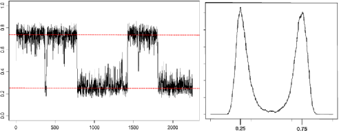
Figure 1: Sample path $X_{N}(t)$ (left: $x$-axis${}=t$, $y$-axis${}=X_{N}(t)=N^{-1}X(t)$) and its occupation density (right: $x$-axis${}={}$state space of $X_{N}\subset[0,1]$, $y$-axis${}={}$proportion of time $X_{N}$ spends in each state by time $t=2500$) from the system (25)–(28) with birth–death splitting, under standard mass-action scaling for reactions and $\gamma(\varepsilon,N)=\frac{1}{2}\varepsilon^{2}N^{2}$ (parameters $N=1500$, $\varepsilon^{2}=0.02$). Dashed red lines indicate quasi-equilibria at $1/4$ and $3/4$.

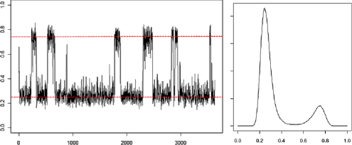
Figure 2: Sample path $X_{N}(t)$ [left: $x$-axis${}=t$, $y$-axis${}=X_{N}(t)$] and its occupation density (right: $x$-axis${}={}$state space of $X_{N}\subset[0,1]$, $y$-axis${}={}$proportion of time $X_{N}$ spends in each state by time $t=4000$) for the system (25)–(28) with birth–death splitting, under standard mass-action scaling for reactions and $\gamma(\varepsilon,N)=\frac{1}{2}\varepsilon^{2}N^{2}$ (parameters $N=500$, $\varepsilon^{2}=2\times 10^{-4}$). Dashed red lines indicate quasi-equilibria at $1/4$ and $3/4$ as above.

If we take $\varepsilon^{2}\ll 1/N$, then transitions between stable equilibria are based only on the scaled rates for the reaction system (25)–(28),

$$\tilde{r}_{+}(x)=1-x+\tfrac{32}{3}x^{2}(1-x)\quad\mbox{and}\quad\tilde{r}_{-}(x)=x+\tfrac{16}{3}x(1-x).$$

By Proposition 3.3 the values of the quasipotential for the birth–death Markov process are

$$\imath_{x_{1},x_{2}}=\int_{x_{1}}^{x_{2}}\ln\biggl{(}\frac{\tilde{r}_{-}(x)}{\tilde{r}_{+}(x)}\biggr{)}\,dx=\int_{{1}/4}^{{1}/2}\ln\biggl{(}\frac{x+({16}/{3})x(1-x)}{1-x+({32}/{3})x^{2}(1-x)}\biggr{)}\,dx\stackrel{{\scriptstyle\cdot}}{{=}}0.006713$$

and

$$\imath_{x_{3},x_{2}}=\int_{x_{3}}^{x_{2}}\ln\biggl{(}\frac{\tilde{r}_{-}(x)}{\tilde{r}_{+}(x)}\biggr{)}\,dx\stackrel{{\scriptstyle\cdot}}{{=}}0.005534.$$

Note that here the values for the quasipotential are no longer equal, and the process will take longer to get out of the neighborhood of the equilibrium $x_{1}=\frac{1}{4}$. Figure 2 shows a simulation of a sample path of the rescaled process $X_{N}$ for $\gamma(N)=\varepsilon^{2}N$ with the choice of parameters $N=500$, but $\varepsilon^{2}=2\times 10^{-4}$. In this case $1/N\gg\varepsilon^{2}$ and we expect the transitions to be due to noise from the reactions arising from finite-$N$ effects. Based on the above calculation we expect the process to be switching away from $B_{0.1}(x_{1})$ at rate $R=e^{-N\imath_{x_{1},x_{2}}}=e^{-3.356629}\stackrel{{\scriptstyle\cdot}}{{=}}0.035$ and away from $B_{0.1}(x_{3})$ at a rate $R^{\prime}=e^{-N\imath_{x_{3},x_{2}}}=e^{-2.769957}\stackrel{{\scriptstyle\cdot}}{{=}}0.062$; indeed, the time spent near $x_{1}$ is appreciably larger than the time spent near $x_{3}$.

We make a particular note that the reaction system considered here is very sensitive to the exact values given for the reaction constants; a small change in these would preserve the double-well potential, but would lead to nonequal depth of the two wells for the quasipotential, and hence instead of a limiting bistable behavior would lead to a limiting metastable behavior as in case (i) of Proposition 3.2. In the next section we discuss the conditions on the scaling of the reaction and splitting/resampling which yield behavior that can also be described as bistable, but where the underlying mechanism is qualitatively different and the restrictions on the reaction system are negligible.

4 Bistable behavior from fast splitting

We next consider the case $\varepsilon_{A}\approx\infty$, and assume that time has been rescaled so that $\tilde{c}_{\sigma^{2}}=\lim_{N\to\infty}c_{\sigma^{2}}(N)\in(0,\infty)$ and $\tilde{c}_{\mu}=\lim_{N\to\infty}c_{\mu}(N)\approx 0$. This is a more unconventional scaling, in which the noise (from balanced reactions and splitting) overwhelms the contribution due to the drift (from biased reactions).

One way to model this with a diffusion would be to introduce a time-scale separation with an additional small parameter $\varepsilon$ in the scaling of all reactions rather than in the rate of splitting. Suppose all reaction constants scale as $\kappa_{\zeta}^{ab}=\varepsilon\tilde{\kappa}_{\zeta}^{ab}N^{1-(a+b)}$, while the rate of splitting $\gamma(x,N)$ satisfies assumption (${7}^{*}$). For any fixed $\varepsilon>0$, the resulting limit of the rescaled process $X_{N}$ would be

$$d\tilde{X}^{\varepsilon}(t)=\varepsilon\tilde{\phi}\bigl{(}\tilde{X}^{\varepsilon}(t)\bigr{)}\,dt+\tilde{\gamma}\tilde{\sigma}\bigl{(}\tilde{X}^{\varepsilon}(t)\bigr{)}\,dB(t),\qquad\tilde{X}^{\varepsilon}\in[0,1],$$ (33)

where $B$ is a standard Brownian motion, and we have the case of a diffusion with a small drift. Note that although $\tilde{\sigma}^{2}(0)=\tilde{\sigma}^{2}(1)=0$ [by assumption (7)], the boundaries $\{0,1\}$ are not absorbing, since there is at least one biased reaction that allows escape from either boundary $\tilde{\phi}(0)>0,\tilde{\phi}(1)<0$ [by assumption (2)]. Other than at the boundaries the contribution of the drift is essentially negligible, and $\tilde{X}^{\varepsilon}$ is approximately a martingale. Most attempts to escape a boundary are followed by the return to the same boundary point; only some end up at the opposite one. In the limit as $\varepsilon\to 0$, the rate of escapes from the boundaries for $\tilde{X}^{\varepsilon}$ vanishes, and there is no switching.

However, under the right conditions, the limit of the original rescaled process will spend almost all of its time at one boundary or the other, switching between the two on a reasonable time-scale, creating again a bistable system. How the effect of the attempts to escape the boundary appears in the limit depends on the rate of the attempts, and the time spent between the boundaries. In order to make a precise statement we need to examine the behavior of the rescaled process $X_{N}$ directly and specify a general set of conditions for a Markov jump process to exhibit this type of switching behavior.

4.1 Stochastic switching

The unscaled process $X_{A}$ is a Markov chain on $\{0,1,\ldots,N\}$ with transitions that are due to the reactions $(a,b,\zeta)\in\mathcal{I}$, as well as the splitting mechanism with distribution $p_{x,y},{(x,y)\in\{0,1,\ldots,N\}^{2}}$. The rates of these transitions from $X_{A}=x$ are equal to $\sum_{(a,b,\zeta)\in\mathcal{I}}\lambda_{\zeta}^{ab}(x)=\sum_{(a,b,\zeta)\in\mathcal{I}}\kappa_{\zeta}^{ab}(N)(x)_{a}(N-x)_{b}$ from the reaction system and $\gamma(x,N)$ from the splitting, respectively. We denote the total combined rate of $X_{A}$ from $i\in\{0,\ldots,n\}$ to $j\in\{0,\ldots,n\}$ by

$$r_{ij}=\sum_{(a,b,j-i)\in\mathcal{I}}\kappa_{j-i}^{ab}(N)i_{a}(N-i)_{b}+\gamma(i,N)p_{i,j}.$$

Transitions due to splitting can have jumps whose size can in principle be as large as $N-1$ (such as those of the Wright–Fisher splitting process example in Section 2.2), although with very small probability. However, a splitting mechanism is absorbing at $\{0,N\}$, $p_{0,0}=p_{N,N}=1$, and the rates of jumps off the boundaries $x\in\{0,N\}$ are created by reactions using only molecules of $B$ (for $x=0$), or using only molecules of $A$ (for $x=N$), with rates

$$r_{0j}=\sum_{(0,b,j)\in\mathcal{I}}\kappa_{j}^{0j}(N)(N)_{b},\qquad r_{Nj}=\sum_{(a,0,N-j)\in\mathcal{I}}\kappa_{N-j}^{a0}(N)(N)_{a}.$$

By assumption (2) in Section 2.1, there exist $j,j^{\prime}\in\{1,\ldots,N-1\}$ such that $r_{0j},r_{Nj^{\prime}}\neq 0$. The leading powers of $N$, $\max_{(0,b,j)\in\mathcal{I}}\{b\}>0$ and$\max_{(a,0,N-j)\in\mathcal{I}}\{a\}>0$, respectively, will determine the rate at which attempts to counteract absorption at the boundaries happen, and in particular, this implies that $r_{0j}$, $r_{Nj}\to\infty$ as $N\to\infty$ [allowing for upcoming condition (34)].

Define an excursion of $X_{A}$ to be any segment $X_{A}(t),t\in[t_{1},t_{2})$ such that $X_{A}(t_{1}-),X_{A}(t_{2})\in\{0,N\}$ and $X_{A}(t)\notin\{0,N\}$ for $t\in[t_{1},t_{2})$. Call an excursion on $[t_{1},t_{2})$ “successful” if $X_{A}(t_{1}-)\neq X_{A}(t_{2})$, and “unsuccessful” otherwise. For $0\leq j\leq N$, let $\tau_{j}:=\inf\{t\geq 0\dvtx X_{A}(t)=j\}$ be the first hitting time of state $j$, and let $\tau_{0,N}=\tau_{0}\land\tau_{N}$ denote the first hitting time of either boundary state. Let

$$e_{j0} = \mathbf{E}\bigl{[}\tau_{0,N}|X_{A}(0)=j,X_{A}(\tau_{0,N})=0\bigr{]},$$

$$e_{jN} = \mathbf{E}\bigl{[}\tau_{0,N}|X_{A}(0)=j,X_{A}(\tau_{0,N})=N\bigr{]}$$

be the expected hitting time of the two boundaries from $j$ and $\pi_{jN}$ be the probability that an excursion from $j$ hits the $N$ boundary first

$$\pi_{jN}=\mathbf{P}\bigl{[}X_{A}(\tau_{0,N})=N|X_{A}(0)=j\bigr{]},$$

and thus $\pi_{j0}=1-\pi_{jN}$ is the probability it first hits the $0$ boundary. The values of $\{e_{j\cdot},\pi_{jN}\}_{j\in\{1,\ldots,N-1\}}$ can be determined by setting up and solving the appropriate linear functionals of the generator for the Markov process $X_{A}$; explicit expressions, however, may be hard to come by for general processes.

Excursions of $X_{A}$ depend on transitions from both reactions and the splitting mechanism. However, if the noise overwhelms the drift, then at each step in the interior transition rates are dominated by those from the balanced reactions and the splitting mechanism. In particular, this will imply that in the interior $X_{A}$ behaves approximately like a martingale, and will allow us to approximate the probability of switching from one boundary point to the other in terms of the relative rates of biased reactions versus balanced reactions and splitting. We will estimate $e_{j0},e_{jN},\pi_{jN}$ in an example to come, and exhibit more explicit conditions than the ones below in the case when the reactions and splitting yield a birth–death process for $X_{A}$.

We first state general conditions under which the rescaled process $X_{N}=X_{A}/N$ can be approximated by a simple Markov jump process. Suppose that there exists two scaling parameters: the order of magnitude of the rate of reactions on the boundary $\omega_{N}\to\infty$, and a time scaling parameter $\beta_{N}>0$ for the rescaled process $X_{N}$, such that

$$\frac{1}{\omega_{N}}\sum_{j}r_{0j}\to\tilde{r}_{+},\qquad\frac{1}{\omega_{N}}\sum_{j}r_{Nj}\to\tilde{r}_{-},$$ (34)

$$\beta_{N}\sum_{j}r_{0j}\pi_{jN}\to\tilde{r}_{01},\qquad\beta_{N}\sum_{j}r_{Nj}\pi_{j0}\to\tilde{r}_{10},$$ (35)

$$\frac{1}{\beta_{N}\omega_{N}}\sum_{j}r_{0j}e_{jN},\qquad\sum_{j}r_{0j}e_{j0},$$

(36)

$$\frac{1}{\beta_{N}\omega_{N}}\sum_{j}r_{Nj}e_{j0},\qquad\sum_{j}r_{Nj}e_{jN}\to 0,$$

with $\tilde{r}_{+},\tilde{r}_{-},\tilde{r}_{01},\tilde{r}_{10}\in(0,\infty)$. Since $r_{0j},r_{Nj}\to\infty$, there is no need to change the time-scale for the process. These conditions imply that there are many excursions in any finite time interval $[0,t]$, only a small fraction of which are successful, and during which the total time spent is very small. Consequently, the rescaled process will spend most of its time on one boundary until the first time a successful excursion takes it to the other boundary. Let $\tilde{T}_{N}^{0}=\inf\{t\geq 0\dvtx X_{A}(t)=0\}$, and

$$T_{N}^{i}=\inf\bigl{\{}t>\tilde{T}_{N}^{i-1}\dvtx X_{A}(t)=N\bigr{\}},\qquad\tilde{T}_{N}^{i}=\inf\bigl{\{}t>T_{N}^{i}\dvtx X_{A}(t)=0\bigr{\}},$$

$$\eqntext{i=1,2\ldots}$$ (37)

be a sequence of times at which $X_{A}$ first reaches a boundary different from the one where it was most recently. Also, define the measure-valued process $(\nu^{N}_{t})_{t\geq 0}$ for some $\rho_{N}>0$ such that $\frac{\rho_{N}}{\beta_{N}}\to 0$ by

$$\nu^{N}_{t}(f)=\frac{1}{\rho_{N}}\int_{\beta_{N}t}^{\beta_{N}t+\rho_{N}}f\bigl{(}X_{N}(s)\bigr{)}\,ds$$

for any (bounded continuous) function $f$ on $\{0,\frac{1}{N},\ldots,1\}$; this $(\nu_{t}^{N})$ approximates the law of the location of the rescaled process $X_{N}(t)=X_{A}(t)/N$ on a short time interval of length $\rho_{N}$.

Proposition 4.1.

If $X_{A}$ satisfies (34)–(4.1), then

$$\lim_{N\to\infty}\mathbf{P}\bigl{[}T_{N}^{i}-\tilde{T}_{N}^{i-1}>t\beta_{N}\bigr{]}=e^{-\tilde{r}_{01}t},\qquad\lim_{N\to\infty}\mathbf{P}\bigl{[}T_{N}^{i+1}-\tilde{T}_{N}^{i}>t\beta_{N}\bigr{]}=e^{-\tilde{r}_{10}t}$$

$$\eqntext{\forall t>0,}$$ (38)

and we have convergence in law on the space of cadlag paths (with the Skorokhod topology) $(\nu^{N}_{t})_{t\geq 0}\Rightarrow(\nu_{t})_{t\geq 0}$ to a jump process

$$\nu_{t}=\cases{\delta_{0},&\quad$T_{2i}\leq t<T_{2i+1},$\vspace*{2pt}\cr\delta_{1},&\quad$T_{2i+1}\leq t<T_{2i+2},$}\qquad i=0,1,2,\ldots,$$

where $\{T_{2i+1}-T_{2i}\}_{i\geq 0}$ and $\{T_{2i+2}-T_{2i+1}\}_{i\geq 0}$ are two independent sequences of i.i.d. exponential variables with rates $\tilde{r}_{01}$ and $\tilde{r}_{10}$, respectively.

The rescaled process $X_{N}$ can therefore be approximated by a jump Markov process $(J(t))_{t\geq 0}$ on $\{0,1\}$ with transition rates $\tilde{r}_{01}$ from ${0\to 1}$, and $\tilde{r}_{10}$ from $1\to 0$ in the following sense: the occupation times of $X_{N}$ on $\{0,1\}$ converge to the respective occupation times of $J$, and the times of successful excursions of $X_{N}$ from $0\to 1$ and from $1\to 0$ converge to the respective transitions of $J$. We cannot expect a stronger kind of convergence than stated, since, for example, convergence in law of $X_{N}$ to $J$ in the Skorokhod topology is precluded by the fact that for arbitrarily large $N$, there remain unsuccessful excursions of $X_{N}$ that stray from their originating boundary by a distance which is bounded away from $0$.

A different set of conditions from those in (4.1) for the length of excursions away from the boundaries, where in the limit we get four nonzero limiting constants $\tilde{e}_{01},\tilde{e}_{00},\tilde{e}_{10},\tilde{e}_{11}$, would imply convergence to a limiting process which spends a nontrivial fraction of time away from the boundary. The limiting process would behave similar to a diffusion with “sticky” boundaries; see KT , Section 15.8C.

Proof of Proposition 4.1 For each $i\geq 0$, define a sequence of times after $\tilde{T}_{N}^{i}$ at which excursions from $0$ start $\tilde{\sigma}_{N}^{i,i^{\prime}}$ and end $\tilde{\tau}_{N}^{i,i^{\prime}}$, by letting $\tilde{\tau}_{N}^{i,0}=\tilde{T}_{N}^{i}$, and for $i^{\prime}=1,2,\ldots$

$$\tilde{\sigma}_{N}^{i,i^{\prime}} = \inf\bigl{\{}\tilde{\tau}_{N}^{i,i^{\prime}-1}<t\dvtx X_{A}(t)\neq 0,X_{A}(t-)=0\bigr{\}},$$

$$\tilde{\tau}_{N}^{i,i^{\prime}} = \inf\bigl{\{}\tilde{\tau}_{N}^{i,i^{\prime}-1}<t\dvtx X_{A}(t)=0,X_{A}(t-)\neq 0\bigr{\}}$$

and let $s(i)=\inf\{i^{\prime}\geq 1\dvtx\tilde{\tau}_{N}^{i,i^{\prime}}>T_{N}^{i+1}\}$ be the index of the first excursion from $0$ that is successful, hence $\tilde{\tau}_{N}^{i,s(i)}=\tilde{T}^{i+1}_{N}$. Note that $X_{A}(t)=0,\forall t\in[\tilde{\tau}_{N}^{i,i^{\prime}-1},\tilde{\sigma}_{N}^{i,i^{\prime}})$ and that $\sum_{i^{\prime}\leq s(i)}(\tilde{\sigma}_{N}^{i,i^{\prime}}-\tilde{\tau}_{N}^{i,i^{\prime}-1})$ is the time spent at $0$ between successful excursions, while $X_{A}\neq 0$ for $t\in[\tilde{\sigma}_{N}^{i,i^{\prime}},\tilde{\tau}_{N}^{i,i^{\prime}})$, and thus $\sum_{i^{\prime}<s(i)}(\tilde{\tau}_{N}^{i,i^{\prime}}-\tilde{\sigma}_{N}^{i,i^{\prime}})$ is the time spent on unsuccessful excursions.

Consider the time interval $[\tilde{T}_{N}^{i},T_{N}^{i+1}]-\bigcup_{i^{\prime}<s(i)}[\tilde{\sigma}_{N}^{i,i^{\prime}},\tilde{\tau}_{N}^{i,i^{\prime}})$ from which subintervals for unsuccessful excursions are excised. Excursions from $0$ are started at overall rate $\sum_{j^{\prime}}r_{0j^{\prime}}$, and since excursions whose first step is to $j$ are successful with probability $\pi_{jN}$, successful excursions are started at rate $\sum_{j}r_{0j}\pi_{jN}$. So

$$W_{N}^{i}:=\tilde{\sigma}_{N}^{i,s(i)}-\tilde{T}_{N}^{i}-\sum_{i^{\prime}<s(i)}\bigl{(}\tilde{\tau}_{N}^{i,i^{\prime}}-\tilde{\sigma}_{N}^{i,i^{\prime}}\bigr{)}\sim\operatorname{exponential}\biggl{(}\sum_{j}r_{0j}\pi_{jN}\biggr{)}$$

and

$$s(i)\sim\operatorname{geometric}\biggl{(}\frac{\sum_{j}r_{0j}\pi_{jN}}{\sum_{j}r_{0j}}\biggr{)}.$$

Also, for any $i^{\prime}<s(i)$, the unsuccessful excursion times $\tilde{\tau}_{N}^{i,i^{\prime}}-\tilde{\sigma}_{N}^{i,i^{\prime}}$ are independent and identically distributed with

$$\mathbf{E}\bigl{[}\tilde{\tau}_{N}^{i,i^{\prime}}-\tilde{\sigma}_{N}^{i,i^{\prime}}\bigr{]}=\sum_{j}\frac{r_{0j}}{\sum_{j^{\prime}}r_{0j^{\prime}}}\mathbf{E}\bigl{[}\tau_{0,N}|X_{A}(0)=j,X_{A}(\tau_{0,N})=0\bigr{]},$$

while $T_{N}^{i+1}-\tilde{\sigma}_{N}^{i,s(i)}$ is a subinterval for a successful excursion with

$$\mathbf{E}\bigl{[}T_{N}^{i+1}-\tilde{\sigma}_{N}^{i,s(i)}\bigr{]}=\sum_{j}\frac{r_{0j}}{\sum_{j^{\prime}}r_{0j^{\prime}}}\mathbf{E}\bigl{[}\tau_{0,N}|X_{A}(0)=j,X_{A}(\tau_{0,N})=N\bigr{]}.$$

Let

$$U_{N}^{i}:=\sum_{i^{\prime}<s(i)}\bigl{(}\tilde{\tau}_{N}^{i,i^{\prime}}-\tilde{\sigma}_{N}^{i,i^{\prime}}\bigr{)}\quad\mbox{and}\quad S_{N}^{i}:=T_{N}^{i+1}-\tilde{\sigma}_{N}^{i,s(i)},$$

so that $T_{N}^{i+1}-\tilde{T}_{N}^{i}=W_{N}^{i}+U_{N}^{i}+S_{N}^{i}$. Assumption (35) implies $W_{N}^{i}/\beta_{N}\Rightarrow\operatorname{exponential}(\tilde{r}_{01}$) as $N\to\infty$. We next show convergence for both $U_{N}^{i}\mathop{\to}0$ and $S_{N}^{i}\mathop{\to}0$ in probability as $N\to\infty$, which will imply that $(T_{N}^{i+1}-\tilde{T}_{N}^{i})/\beta_{N}\Rightarrow\operatorname{exponential}(\tilde{r}_{01}$).

We first note that

$$\mathbf{E}\bigl{[}S_{N}^{i}\bigr{]} = \mathbf{E}\bigl{[}T_{N}^{i+1}-\tilde{\sigma}_{N}^{i,s(i)}\bigr{]}=\sum_{j}\frac{r_{0j}}{\sum_{j^{\prime}}r_{0j^{\prime}}}e_{jN}$$

$$= \frac{1}{\sum_{j^{\prime}}(r_{0j^{\prime}}/\omega_{N})}\frac{1}{\beta_{N}\omega_{N}}\sum_{j}r_{0j}e_{jN}\cdot\beta_{N};$$

therefore, $\mathbf{E}[S_{N}^{i}/\beta_{N}]\to 0$, since the first fraction converges to $1/\tilde{r}_{+}$, and the second to $0$, by (34) and (4.1), respectively. Similarly, for each unsuccessful excursion $1\leq i^{\prime}<s(i)$

$$\mathbf{E}\bigl{[}\tilde{\tau}_{N}^{i,i^{\prime}}-\tilde{\sigma}_{N}^{i,i^{\prime}}\bigr{]}=\frac{1}{\omega_{N}}\frac{1}{\sum_{j^{\prime}}(r_{0j^{\prime}}/\omega_{N})}\sum_{j}r_{0j}e_{j0},$$

and since $s(i)$ is geometric,

$$\mathbf{E}\bigl{[}s(i)\bigr{]}=\frac{\sum_{j}r_{0j}}{\sum_{j}r_{0j}\pi_{jN}}={\omega_{N}}\frac{\sum_{j}r_{0j}/\omega_{N}}{\sum_{j}r_{0j}\pi_{jN}}.$$

We have

$$\mathbf{E}\bigl{[}U_{N}^{i}\bigr{]}=\mathbf{E}\biggl{[}\sum_{i^{\prime}<s(i)}\bigl{(}\tilde{\tau}_{N}^{i,i^{\prime}}-\tilde{\sigma}_{N}^{i,i^{\prime}}\bigr{)}\biggr{]}\leq\mathbf{E}\bigl{[}s(i)\bigr{]}\mathbf{E}\bigl{[}\tilde{\tau}_{N}^{i,i^{\prime}}-\tilde{\sigma}_{N}^{i,i^{\prime}}\bigr{]}=\frac{\sum_{j}r_{0j}e_{j0}}{\beta_{N}\sum_{j}r_{0j}\pi_{jN}}\cdot\beta_{N}$$

and so $\mathbf{E}[U_{N}^{i}/\beta_{N}]\to 0$, since by (35) the denominator converges to $\tilde{r}_{01}$, and by (4.1) the numerator goes to $0$. Hence for any $\delta>0$ we have $\mathbf{P}[S_{N}^{i}>\delta]\leq\frac{\mathbf{E}[S_{N}^{i}]}{\delta}\to 0$ and $\mathbf{P}[U_{N}^{i}>\delta]\leq\frac{\mathbf{E}[U_{N}^{i}]}{\delta}\to 0$.

A completely analogous proof shows that $(\tilde{T}_{N}^{i}-T_{N}^{i})\beta_{N}\Rightarrow\operatorname{exponential}(\tilde{r}_{10}$), and the claim about the probability measure $\nu_{t}$ is immediate from the fact that $\mathbf{E}[U_{N}^{i}+S_{N}^{i}]\to 0$.

To verify condition (34) one only needs to use the rates of biased reactions on the boundary. For (35), note the fact that if not for biased reactions, the process would be a martingale; if the rates of the biased reactions are overpowered by those of the balanced reactions and splitting [as quantified in (35)], then the process is approximately a martingale. Conditions in (4.1) predominantly depend on how fast the rates of the balanced reactions and splitting are, as they determine the length of excursions of the process.

These conditions are the easiest to verify when the reactions as well as splitting/resampling mechanism make only unit net changes at each step, so that $X_{A}$ is a birth–death process with $r_{ij}=0$ if $|i-j|>1$. In this case one can specify more precise conditions on the rates $r_{ij}$ that will ensure that (34)–(4.1) hold. We consider the case when the time is already rescaled, that is, $\beta_{N}=1$, and the rate of reactions on the boundaries is $\omega_{N}=N$. We use the following notation for birth and death rates:

$$r_{+}(i):=r_{i(i+1)},\qquad r_{-}(i):=r_{i(i-1)},\qquad\varepsilon_{N}(i)=\frac{r_{-}(i)}{r_{+}(i)}-1,$$

with $\varepsilon_{N}(i)$ quantifying the strength of the bias at state $i$ [we stress its dependence on $N$ via transition rates $r_{\pm}(i)$].

Proposition 4.2.

If $X_{A}$ is a birth–death chain whose rates satisfy

$$\frac{r_{+}(0)}{N} \to \tilde{r}_{+}\in(0,\infty),\qquad\frac{r_{-}(N)}{N}\to\tilde{r}_{-}\in(0,\infty),$$ (39)

$$\sum_{i=1}^{N-1}\bigl{|}\varepsilon_{N}(i)\bigr{|} \to 0\quad\mbox{and}$$ (40)

$$\sum_{i=1}^{N-1}\frac{N-i}{r_{+}(i)} \to 0,\qquad\sum_{i=1}^{N-1}\frac{i}{r_{-}(i)}\to 0,$$ (41)

then conditions (34)–(4.1) hold with $\omega_{N}=N$, $\beta_{N}=1$ and $\tilde{r}_{01}=\tilde{r}_{+}$, $\tilde{r}_{10}=\tilde{r}_{-}$.

Analogous to the general case, (39) depends only on the rates of biased reactions on the boundaries, (40) reflects the fact that off of the boundaries the drift of the biased reactions is much weaker than the noise of the balanced reactions and splitting and (41) is an estimate on the speed of the balanced reactions and splitting.

Proof of Proposition 4.2 (34) is immediate from (39) and $\omega_{N}=N$. To verify (35) we solve for $\pi_{jN},j\in\{1,\ldots,N-1\}$.

Lemma 4.1.

If (40) holds, then $N\pi_{1N}\to 1$ and $N\pi_{(N-1)0}\to 1$.

Let $\varphi$ be such that $\varphi(X_{A})$ is a martingale, that is, let $\varphi(x)=\mathbf{E}[\varphi(X_{A}(\tau_{0,N}))|X(0)=x]$ for $x\in\{1,\ldots,N-1\}$ and $\varphi(0)=0,\varphi(1)=1$. Standard result for birth–death processes, using a recursive equation for $\psi(x)=\varphi(x)-\varphi(x-1)$, gives

$$\varphi(x)=\sum_{i=1}^{x}\psi(i)=\sum_{i=1}^{x}\prod_{j=1}^{i-1}\frac{r_{-}(j)}{r_{+}(j)}.$$

By the optional stopping theorem for the stopping time $\tau_{0,N}$,

$$\varphi(i)=\mathbf{E}\bigl{[}\varphi\bigl{(}X_{A}(\tau_{0,N})\bigr{)}|X(0)=i\bigr{]}=\pi_{i0}\varphi(0)+\pi_{iN}\varphi(N),$$

so $\pi_{iN}={(\varphi(i)-\varphi(0))}/{(\varphi(N)-\varphi(0))}=\varphi(i)/\varphi(N)$, and

$$\pi_{1N}=\frac{1}{\varphi(N)}=\Biggl{(}\sum_{i=1}^{N}\prod_{j=1}^{i-1}\frac{r_{-}(j)}{r_{+}(j)}\Biggr{)}^{-1}=\Biggl{(}\sum_{i=1}^{N}\prod_{j=1}^{i-1}\bigl{(}1+\varepsilon_{N}(j)\bigr{)}\Biggr{)}^{-1}=\frac{1}{Nc(N)},$$

where $c(N)=\frac{1}{N}\sum_{i=1}^{N}\prod_{j=1}^{i-1}(1+\varepsilon_{N}(j))$.

Condition (40) implies that $\sup_{1\leq j\leq N-1}\{|\varepsilon_{N}(j)|\}\to 0$, so let $N_{0}$ be such that $\forall N>N_{0}$ and $\forall j\in\{1,\ldots,N-1\}$, $|\varepsilon_{N}(j)|<1/3$. Since $\forall x\in[0,1/3),1-x\geq e^{-x-x^{2}}$, and $\forall x\in\mathbb{R},1+x\leq e^{x}$, we have that uniformly for all $1\leq a,b\leq N-1$, where $N>N_{0}$

$$\qquad\prod_{j=a}^{b}\bigl{(}1+\varepsilon_{N}(j)\bigr{)}\leq\prod_{j=1}^{N-1}\bigl{(}1+\bigl{|}\varepsilon_{N}(j)\bigr{|}\bigr{)}\leq\prod_{j=1}^{N-1}e^{|\varepsilon_{N}(j)|}=\exp\Biggl{(}\sum_{j=1}^{N-1}\bigl{|}\varepsilon_{N}(j)\bigr{|}\Biggr{)}$$ (42)

and

$$\prod_{j=a}^{b}\bigl{(}1+\varepsilon_{N}(j)\bigr{)} \geq \prod_{j=a}^{b}\bigl{(}1-\bigl{|}\varepsilon_{N}(j)\bigr{|}\bigr{)}\geq\prod_{j=1}^{N-1}\bigl{(}1-\bigl{|}\varepsilon_{N}(j)\bigr{|}\bigr{)}$$

$$\geq \prod_{j=1}^{N-1}\exp\bigl{(}-\bigl{|}\varepsilon_{N}(j)\bigr{|}-\bigl{|}\varepsilon_{N}(j)\bigr{|}^{2}\bigr{)}$$

$$= \exp\Biggl{(}-\sum_{j=1}^{N-1}\bigl{(}\bigl{|}\varepsilon_{N}(j)\bigr{|}+\bigl{|}\varepsilon_{N}(j)\bigr{|}^{2}\bigr{)}\Biggr{)}$$

hence $N\pi_{1N}=1/c(N)\to 1$.

To get $N\pi_{(N-1)0}\to 1$, if we flip the state space by letting $\check{\iota}=N-i$, then the new boundaries are $\check{0}=N$ and $\check{N}=0$, and we get a birth–death process $\check{X}_{A}$ whose rates are precisely the flip of those for $X_{A}$. That is, the rates of $\check{X}_{A}$ are $\check{r}_{+}(\check{\iota})=r_{-}(N-i)$, $\check{r}_{-}(\check{\iota})=r_{+}(N-i)$, and their ratio is

$$1+\check{\varepsilon}_{N}({\check{\iota}})=\frac{\check{r}_{-}(\check{\iota})}{\check{r}_{+}(\check{\iota})}=\frac{r_{+}(N-i)}{r_{-}(N-i)},$$

giving the same product of ratios as for the original process.

$$\prod_{\check{\iota}=1}^{N-1}\bigl{(}1+\check{\varepsilon}_{N}({\check{\iota}})\bigr{)}=\prod_{j=1}^{N-1}\bigl{(}1+\varepsilon_{N}(j)\bigr{)}.$$

Hence, the exact argument above now applied to $\check{X}_{A}$ gives $N\check{\pi}_{\check{1}\check{N}}=\break N\pi_{(N-1)0}\to 1$ as well.

Once we have the result of Lemma 4.1, it is immediate that $N\pi_{1N}\to 1,N\pi_{(N-1)0}$ imply (35) with $\tilde{r}_{01}=\tilde{r}_{+},\tilde{r}_{10}=\tilde{r}_{-}$.

To verify (4.1) we next solve for $e_{j},j\in\{1,\ldots,N-1\}$, where $e_{j}=\mathbf{E}[\tau_{0,N}|\break X_{A}(0)=j]$ for $j\in\{1,\ldots,N-1\}$, and $e_{0}=e_{N}=0$.

Lemma 4.2.

If (40) and (41) hold, then $Ne_{1}\to 0$ and $Ne_{N-1}\to 0$.

The expected time of an excursion satisfies the recursion

$$e_{i}=\frac{1}{r_{-}(i)+r_{+}(i)}+\frac{r_{-}(i)}{r_{-}(i)+r_{+}(i)}e_{i-1}+\frac{r_{+}(i)}{r_{-}(i)+r_{+}(i)}e_{i+1},$$

which gives

$$r_{+}(i)(e_{i+1}-e_{i})-r_{-}(i)(e_{i}-e_{i-1})=-1;$$

letting $f(i)=e_{i}-e_{i-1}$ gives the recursive equation

$$f(i+1)=-\frac{1}{r_{+}(i)}+\frac{r_{-}(i)}{r_{+}(i)}f(i)=-\frac{1}{r_{+}(i)}+\bigl{(}1+\varepsilon_{N}(i)\bigr{)}f(i).$$

Note that except for the $-\frac{1}{r_{+}(i)}$ term, this is reminiscent of the recursion for $\psi(i)=\frac{r_{-}(i)}{r_{+}(i)}\psi(i-1)$. Hence

$$f(k)=f(1)\prod_{j=1}^{k-1}\bigl{(}1+\varepsilon_{N}(j)\bigr{)}-\sum_{i=1}^{k-1}\frac{1}{r_{+}(i)}\prod_{j=i+1}^{k-1}\bigl{(}1+\varepsilon_{N}(j)\bigr{)}.$$

To find $f(1)=e_{1}-e_{0}=e_{1}$ we impose the condition $\sum_{i=1}^{N}f(i)=e_{N}-e_{0}=0$ and get

$$e_{1}=\Biggl{(}\sum_{k=1}^{N}\sum_{i=1}^{k-1}\frac{1}{r_{+}(i)}\prod_{j=i+1}^{k-1}\bigl{(}1+\varepsilon_{N}(j)\bigr{)}\Biggr{)}\bigg{/}\Biggl{(}\sum_{k=1}^{N}\prod_{j=1}^{k-1}\bigl{(}1+\varepsilon_{N}(j)\bigr{)}\Biggr{)}.$$

Let $\eta_{N}=\sup_{1\leq a,b\leq N-1}|\prod_{a}^{b}(1+\varepsilon_{N}(j))-1|$. Then (40) implies $\eta_{N}\to 0$ for $N>N_{0}$ via (42) and (4.1). We have

$$e_{1} \leq \Biggl{(}\sum_{k=1}^{N}\sum_{i=1}^{k-1}\frac{1}{r_{+}(i)}(1+\eta_{N})\Biggr{)}\bigg{/}\Biggl{(}\sum_{k=1}^{N}(1-\eta_{N})\Biggr{)}$$

$$= \frac{1+\eta_{N}}{(1-\eta_{N})N}\sum_{k=1}^{N}\sum_{i=1}^{k-1}\frac{1}{r_{+}(i)}=\frac{1+\eta_{N}}{(1-\eta_{N})N}\sum_{i=1}^{N-1}\frac{N-i}{r_{+}(i)},$$

and thus (41) implies $Ne_{1}\to 0$.

To obtain $Ne_{N-1}\to 0$ we can flip the process and consider $\check{X}_{A}$ with the flipped rates as in the proof of Lemma 4.1. Now, in addition to (40), we also require the flip version of the first condition in (41),

$$\sum_{\check{\iota}=1}^{N-1}\frac{\check{N}-\check{\iota}}{\check{r}_{+}(\check{\iota})}=\sum_{i=1}^{N-1}\frac{N-i}{r_{-}(N-i)}=\sum_{i=1}^{N-1}\frac{i}{r_{-}(i)}\to 0,$$

which are guaranteed by the second condition in (41).

Once we have the results of both Lemmas 4.1 and 4.2, we can deduce that $Ne_{1}\to 0$ and $Ne_{N-1}\to 0$, which imply (4.1). Namely, from $e_{1}=e_{1N}\pi_{1N}+e_{10}\pi_{10}$,

$$e_{1N}\leq\frac{e_{1}}{\pi_{1N}}=\frac{Ne_{1}}{N\pi_{1N}}\to 0$$

since Lemma 4.1 ensures convergence of the denominator to $1$ and Lemma 4.2 of the numerator to 0. Similarly

$$Ne_{10}\leq\frac{Ne_{1}}{\pi_{10}}\leq\frac{Ne_{1}}{r_{-}(0)/(r_{+}(0)+r_{-}(0))}\to 0$$

since $\pi_{10}$ contains the positive probability (independent of $N$) of an immediate return to $0$.

For a reaction system and splitting with unit net changes only, since splitting is unbiased we have $p_{i,i+1}=p_{i,i-1}=\frac{1}{2}$, for $i\neq 0,N$, and the contribution to $r_{+}(i)$ and $r_{-}(i)$ from splitting is $\frac{1}{2}\gamma(i,N)$. Let us write $\gamma(i,N)=\gamma(N)p_{i}$ where $\gamma(N)$ depends on $N$ only (i.e., is state independent) and $p_{i}=O(1)$. Then, in any state, the contribution of the splitting is of $O(\gamma(N))$, while the contribution of the reaction system is of $O(N)$ due to the standard scaling of reaction rates. Hence, we have the following result.

Theorem 4.1.

If the reaction system has increments of size $\{1,-1\}$ only; contains reactions $aA\to(a-1)A+B$, $bB\to A+(b-1)B$ some $a,b>0$; has rates with standard scaling $\kappa^{ab}_{\zeta}(N)=\tilde{\kappa}_{\zeta}^{ab}N^{1-(a+b)}$; and if the splitting mechanism has increments of size $\{1,-1\}$, $p_{0,0}=p_{N,N}=1$, with rate is $\gamma(i,N)=\gamma(N)p_{i}$ where $\gamma(N)$ and $p_{i}=O(1)$ satisfy

$$\qquad\frac{N}{\gamma(N)}\sum_{i=1}^{N-1}\frac{1}{p_{i}}\to 0,\qquad\frac{1}{\gamma(N)}\sum_{i=1}^{N-1}\frac{i}{p_{i}}\to 0,\qquad\frac{1}{\gamma(N)}\sum_{i=1}^{N-1}\frac{N-i}{p_{i}}\to 0;$$ (44)

then the results of Proposition 4.2 apply with $\beta_{N}=1$ and $\tilde{r}_{01}=\sum_{(0,b,1)\in\mathcal{I}}\tilde{\kappa}^{0b}_{1},\break\tilde{r}_{10}=\sum_{(a,0,-1)\in\mathcal{I}}\tilde{\kappa}^{a0}_{-1}$.

The transition rates for $X_{A}$ are given by

$$r_{+}(i) = \frac{1}{2}\gamma(N)p_{i}+N\sum_{(a,b,1)\in\mathcal{I}}\tilde{\kappa}^{ab}_{1}(i/N)_{a,N}(1-i/N)_{b,N},$$

$$\eqntext{i=0,\ldots,N-1,}$$ (45)

$$r_{-}(i) = \frac{1}{2}\gamma(N)p_{i}+N\sum_{(a,b,-1)\in\mathcal{I}}\tilde{\kappa}^{ab}_{-1}(i/N)_{a,N}(1-i/N)_{b,N},\qquad i=1,\ldots,N.$$

On the boundary the rates are

$$r_{+}(0)=N\sum_{(0,b,1)\in\mathcal{I}}\tilde{\kappa}_{1}^{0b},\qquad r_{-}(N)=N\sum_{(a,0,-1)\in\mathcal{I}}\tilde{\kappa}_{-1}^{a0},$$

and (39) holds with $\tilde{r}_{+}=\sum_{(0,b,1)\in\mathcal{I}}\tilde{\kappa}_{1}^{0b},\tilde{r}_{-}=\sum_{(a,0,-1)\in\mathcal{I}}\tilde{\kappa}_{-1}^{a0}$. Also,

$$\varepsilon_{N}(i) = \frac{({1}/2)\gamma(N)p_{i}+N\sum_{(a,b,-1)\in\mathcal{I}}\tilde{\kappa}^{ab}_{-1}(i/N)_{a,N}(1-i/N)_{b,N}}{({1}/2)\gamma(N)p_{i}+N\sum_{(a,b,1)\in\mathcal{I}}\tilde{\kappa}^{ab}_{1}(i/N)_{a,N}(1-i/N)_{b,N}}-1$$

$$= \biggl{(}N\biggl{(}\sum_{(a,b,1)\in\mathcal{I}}\tilde{\kappa}^{ab}_{-1}(i/N)_{a,N}(1-i/N)_{b,N}$$

$$\hskip 20.0pt{}-\sum_{(a,b,1)\in\mathcal{I}}\tilde{\kappa}^{ab}_{1}(i/N)_{a,N}(1-i/N)_{b,N}\biggr{)}\biggr{)}$$

$${}\Big{/}\biggl{(}({1}/2)\gamma(N)p_{i}+N\sum_{(a,b,1)\in\mathcal{I}}\tilde{\kappa}^{ab}_{1}(i/N)_{a,N}(1-i/N)_{b,N}\biggr{)}$$

$$\leq \frac{2NR\max_{(a,b,\zeta)\in\mathcal{I}}\tilde{\kappa}_{\zeta}^{ab}}{\gamma(N)p_{i}}$$

since $\tilde{\kappa}^{ab}_{\zeta}\geq 0$, where $R<\infty$ is the number of reactions in the system. Therefore

$$\sum_{i=1}^{N-1}\bigl{|}\varepsilon_{N}(i)\bigr{|}\leq 2R\max_{(a,b,\zeta)\in\mathcal{I}}\bigl{\{}\tilde{\kappa}_{\zeta}^{ab}\bigr{\}}\frac{N}{\gamma(N)}\sum_{i=1}^{N-1}\frac{1}{p_{i}},$$

and the first condition in (44) ensures that $\sum_{i=1}^{N-1}|\varepsilon_{N}(i)|\to 0$ and (40) holds. On the other hand,

$$\sum_{i=1}^{N-1}\frac{i}{r_{-}(i)} = \sum_{i=1}^{N-1}\frac{i}{({1}/2)\gamma(N)p_{i}+\sum_{(a,b,-1)\in\mathcal{I}}\tilde{\kappa}^{ab}_{-1}(i/N)^{a-1}(1-i/N)^{b}}$$

$$\leq \frac{2}{\gamma(N)}\sum_{i=1}^{N-1}\frac{i}{p_{i}}$$

and

$$\sum_{i=1}^{N-1}\frac{N-i}{r_{+}(i)}\leq\frac{2}{\gamma(N)}\sum_{i=1}^{N-1}\frac{N-i}{p_{i}}$$

so the last two conditions in (44) ensure that (41) is satisfied as well.

4.2 Example: Bistable behavior from fast splitting

We revisit the same example of the reaction system we analyzed in Section 3.3:

$$A \stackrel{{\scriptstyle\kappa^{10}_{-1}}}{{\to}} B,$$ (46)

$$B \stackrel{{\scriptstyle\kappa^{01}_{1}}}{{\to}} A,$$ (47)

$$A+B \stackrel{{\scriptstyle\kappa^{11}_{-1}}}{{\to}} 2B,$$ (48)

$$2A+B \stackrel{{\scriptstyle\kappa^{21}_{1}}}{{\to}} 3A$$ (49)

with the standard mass-action scaling, $\kappa^{ab}_{\zeta}=N^{-(a+b)+1}\tilde{\kappa}^{ab}_{\zeta}$. In this system the only reactions which counteract the absorption on the boundaries are the first two unimolecular reactions. Also, note that all system reactions change the molecular count of $A$ only by increments of size $1$.

We chose the same simple splitting mechanism as before, since conditions (40), (41) and (44) are much easier to verify than conditions (35), (4.1). Recall that, if we were to assume $\gamma(N)=\frac{1}{2}\varepsilon^{2}N^{2}$ for some small $\varepsilon^{2}>0$, then the limiting process for $X_{N}$ would be the diffusion process $\tilde{X}_{\varepsilon}$ in (3.3); the splitting noise is even less present if we were to assume $\gamma(N)=\frac{1}{2}N$, as shown in Section 3.3. In contrast, if we assume the rate $\gamma(N)$ grows fast enough so that $N^{2}\ln{N}/\gamma(N)\to 0$, then we can show that the conditions in Proposition 4.2 are satisfied, and the behavior of the limiting process for $X_{N}$ is described by a different two-state jump Markov process.

There are only two reactions in (46)–(49) active on the boundaries, so $\tilde{r}_{01}=\tilde{\kappa}^{01}_{1}$ and $\tilde{r}_{10}=\tilde{\kappa}^{10}_{-1}$. To verify (44), note that we have $\gamma(i,N)=\gamma(N)p_{i}$ with $p_{i}=\frac{i}{N}(1-\frac{i}{N})={i(N-i)}/{N^{2}}$, so

$$\frac{N}{\gamma(N)}\sum_{i=1}^{N-1}\frac{1}{p_{i}}=\frac{N^{3}}{\gamma(N)}\sum_{i=1}^{N-1}\frac{1}{i(N-i)}=\frac{N^{2}}{\gamma(N)}\sum_{i=1}^{N-1}\biggl{(}\frac{1}{i}+\frac{1}{N-i}\biggr{)}=\frac{2N^{2}h_{N}}{\gamma(N)}$$

using partial fractions $\frac{1}{i(N-i)}=\frac{1}{N}(\frac{1}{i}+\frac{1}{(N-i)})$, where $h_{N}$ is the $N$th harmonic sum. Also

$$\frac{1}{\gamma(N)}\sum_{i=1}^{N-1}\frac{i}{p_{i}}=\frac{N^{2}}{\gamma(N)}\sum_{i=1}^{N-1}\frac{1}{N-i}=\frac{N^{2}h_{N}}{\gamma(N)}$$

and

$$\frac{1}{\gamma(N)}\sum_{i=1}^{N-1}\frac{N-i}{p_{i}}=\frac{1}{\gamma(N)}\sum_{i=1}^{N-1}\frac{1}{i}=\frac{N^{2}h_{N}}{\gamma(N)}$$

as well. Hence, $N^{2}{\ln N}/{\gamma(N)}\to 0$ ensures that all conditions in (44) hold.

This example shows that for any reaction system with unit increments whose drift has a double well potential, and for this particular choice of the splitting mechanism, we can identify orders of magnitude for $\gamma(N)$ that lead to different limiting behaviors:

$\bullet$ If $\gamma(N)\ll N$, bistability is caused by large deviations of the Markov jump process, and the rescaled process transitions between neighborhoods of the drift equilibirum points on a time-scale of order $e^{N(\gamma(N))^{-1}\imath_{x_{i},x_{2}}}$, with $N(\gamma(N))^{-1}\to\infty$.

$\bullet$ If $\gamma(N)\sim\varepsilon^{2}N^{2}$, $\varepsilon^{2}>0$ a constant, bistability is caused by large deviations of a diffusion with a small perturbation coefficient, with transitions between neighborhoods of the drift equilibirum points on a time-scale of order $e^{\varepsilon^{-2}I_{x_{i},x_{2}}}$.

$\bullet$ If $\gamma(N)\gg N^{2}\ln{N}$, bistability is caused by excessive noise, and switching between the boundary points occurs on a time-scale of order $1$.

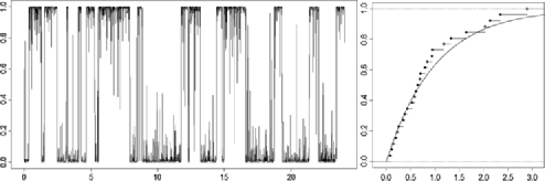
Figure 3: Sample path $X_{N}(t)$ (left: $x$-axis${}=t$, $y$-axis${}=X_{N}(t)=N^{-1}X(t)\subset[0,1]$) of the system (25)–(28) with (31) splitting, under standard mass-action scaling for reactions and $\gamma(N)=\frac{1}{2}N^{3}$ (parameter $N=200$); and the distribution of switching times plotted (dots) in terms of quantiles (right: $x$-axis${}=t$, $y$-axis${}={}$fraction of switching times of length $\leq t$). Solid line ($1-e^{-t}$) indicates the quantiles of the exponential (mean $1$) distribution for comparison.

Note that the order of magnitude $N^{2}$ only represents the scale on which we have assumed that the variance of the splitting mechanism is in the diffusive case [see assumption (${7}^{*}$) in Section 2.2]. Also note that existence of two stable states in the deterministic model for the reaction system is not needed for the result of this section. We chose the same reaction system in order to make the comparison with the results in Section 3 and emphasize the difference between the effects of “slow” and “fast” splitting on the same reaction system.

Figure 3 shows an exact simulation of a sample path of the rescaled process $X_{N}=N^{-1}X_{A}$ for a relatively short period of time, spending most of its time at boundaries $\{0\}\cup\{1\}$, switching between them at approximately rates $\tilde{r}_{01}=\tilde{\kappa}^{01}_{1}=1,\tilde{r}_{10}=\tilde{\kappa}^{10}_{-1}=1$; see Section 3.3 for coefficient values. Switching between states occurs at a time-scale $\beta_{N}=1$, and since $\tilde{r}_{01}=\tilde{\kappa}^{01}_{1}=1,\tilde{r}_{10}=\tilde{\kappa}^{10}_{-1}=1$ the distribution of switching times should approximately be an exponential distribution (mean $1$) distribution. This is shown in the quantile plot in Figure 3, where the fraction of switching times of length $\leq t$ is plotted against the same fraction $1-e^{-t}$ for the exponential (mean $1$) distribution.

5 Discussion

We showed that there are two different types of stochastic bistable behavior in which the system spends most of its time at or near one of two states and switches between them. For one of these types of bistability, because the magnitude of noise is high, it can occur even in a system whose deterministic model would not allow for a possibility of bistability at all. The detreministic system can have unique stable points, as, for example, in the neutral Wright–Fisher model with mutation. For the other type of bistability, where the noise is relatively low, one needs the reaction system to have two deterministic stable points, as, for example, in the Schlögl model. The important point is what constitutes “high” and “low” levels of noise: the determining quantity $\varepsilon_{A}(N)$ (11) depends on the relative size in terms of $N$ of the variance to the average change in the system, where $N$ is a scaling parameter for the size of the system. We referred to $\varepsilon_{A}(N)\approx 0$ as “slow” splitting, and to $\varepsilon_{A}(N)\approx\infty$ as “fast” splitting, interpreted relative to the reaction dynamics.

We discussed the differences in the qualitative signatures of bistability in the two cases:

• In case of “slow” splitting, the states where the process spends most of its time are determined by the drift of the deterministic model for the reaction system; in contrast, in case of “fast” splitting, they are simply the two extremes for the size of the system.

• In case of “slow” splitting, the rate of switching is determined by the relative magnitude of the splitting variance to the reaction drift and by the size of the potential barrier in the deterministic model for the system; on the other hand, in case of “fast” splitting, the rates of switching are determined only by the standardized rates of the reactions that are realizable from one of the extremes for the system size.

• In case of “slow” splitting, the time-scale $\beta_{\varepsilon}$ or $\beta_{\varepsilon_{N}}$ on which the switching happens is exponential in (some increasing function of) the size of the system; in contrast, in case of “fast” splitting, the time-scale $\beta_{N}$ is at most polynomial.

We also showed that the observables of bistability (switching states and rates) are not sensitive to precise specification of the reaction system, as they depend only on: equilibrium points, size of potential barrier in “slow” splitting, and drift values at boundaries in “fast” splitting. However, bistability is very sensitive to the distributional form of the splitting/resampling mechanism: the variance of its distribution determines the potential barrier in “slow” splitting, and the harmonic sum of its transition probabilities determines the threshold for appearance of “fast” splitting.

In the context of cellular systems of biochemical reactions, the problem of determining the partitioning errors due to cell division is experimentally extremely challenging (Huh and Paulsson Pa1 , Pa2 ). The measurements for single cells rely on count estimates for related species rather than the molecular species of interest. In addition, in order to estimate the magnitude of intracellular noise, one has to separate the intrinsic from the extrinsic sources of randomness. How random is cell division, and how it compares in magnitude to the biochemical noise is a question that is very much open. However, since our analysis only depends on a few general features of the splitting mechanism (unbiasedness and time-scale of the rate), it is also possible that stochastic bistability is achieved by a set of auxiliary reactions, instead of splitting, acting on a different time-scale from the rest of the system. For example, the protein bursting mechanism may act as the driver of stochastic bistability (Zong et al. ZSSSG , Kaufman et al. KYMvO ).

One can try to rely on the qualitative signatures of bistability in order to assess which of the two types of bistability we discussed is relevant in a specific cellular biochemical systems. When the switching times are orders of magnitude greater than the molecular count of the switching species, as in the lysogenic switch of E. coli, the “slow” splitting may be the more likely mechanism. This evaluation is sensitive to the choice of time units, given which both the splitting and reaction rates should be of reasonable orders of magnitude in terms of the molecular count. It is natural to chose units of time corresponding to cell-doubling or cell-division time (the splitting rate is then of order 1—and the range of splitting rates in our model, in any of the different cases, is at most linear). In an experimental analysis of this system, Zong et al. ZSSSG observed that the switching times of the cell are exponential in the number of protein burst events, and correspond to a calculation of the rare event probability of the bursts, as can be interpreted by large deviations in our “low” auxiliary noise (“slow” splitting) type of bistability. In contrast, when the switching times are relatively short, as in the gene expression switch in S. cerevisiae, the “fast” splitting is the probable mechanism. In the engineered chemical reaction network version of this system, Kaufmann et al. KYMvO show that increasing the protein burst size (increasing the auxiliary noise) leads to more highly correlated switching behavior in different cell lineages, as could be inferred from properties of our “high” auxiliary noise (“fast” splitting) bistability type.

References

- (1) {barticle}[pbm] \bauthor\bsnmAcar, \bfnmMurat\binitsM., \bauthor\bsnmMettetal, \bfnmJerome T.\binitsJ. T. and \bauthor\bparticlevan \bsnmOudenaarden, \bfnmAlexander\binitsA. (\byear2008). \btitleStochastic switching as a survival strategy in fluctuating environments. \bjournalNat. Genet. \bvolume40\bpages471–475.\biddoi=10.1038/ng.110, issn=1546-1718, pii=ng.110, pmid=18362885\bptokimsref \endbibitem
- (2) {barticle}[pbm] \bauthor\bsnmAvery, \bfnmSimon V.\binitsS. V. (\byear2006). \btitleMicrobial cell individuality and the underlying sources of heterogeneity. \bjournalNat. Rev. Microbiol. \bvolume4 \bpages577–587. \biddoi=10.1038/nrmicro1460, issn=1740-1526, pii=nrmicro1460, pmid=16845428 \bptokimsref \endbibitem
- (3) {barticle}[mr] \bauthor\bsnmBall, \bfnmKaren\binitsK., \bauthor\bsnmKurtz, \bfnmThomas G.\binitsT. G., \bauthor\bsnmPopovic, \bfnmLea\binitsL. and \bauthor\bsnmRempala, \bfnmGreg\binitsG. (\byear2006). \btitleAsymptotic analysis of multiscale approximations to reaction networks. \bjournalAnn. Appl. Probab. \bvolume16 \bpages1925–1961. \biddoi=10.1214/105051606000000420, issn=1050-5164, mr=2288709 \bptokimsref \endbibitem
- (4) {barticle}[auto:STB—2013/10/14—10:36:11] \bauthor\bsnmBishop, \bfnmL. M.\binitsL. M. and \bauthor\bsnmQian, \bfnmH.\binitsH. (\byear2010). \btitleStochastic bistability and bifurcation in a mesoscopic signaling system with autocatalytic kinase. \bjournalBiophysical Journal \bvolume98 \bpages111. \bptokimsref \endbibitem
- (5) {barticle}[pbm] \bauthor\bsnmBrehm-Stecher, \bfnmByron F.\binitsB. F. and \bauthor\bsnmJohnson, \bfnmEric A.\binitsE. A. (\byear2004). \btitleSingle-cell microbiology: Tools, technologies, and applications. \bjournalMicrobiol. Mol. Biol. Rev. \bvolume68 \bpages538–559. \biddoi=10.1128/MMBR.68.3.538-559.2004, issn=1092-2172, pii=68/3/538, pmcid=515252, pmid=15353569 \bptokimsref \endbibitem
- (6) {barticle}[mr] \bauthor\bsnmChvátal, \bfnmV.\binitsV. (\byear1979). \btitleThe tail of the hypergeometric distribution. \bjournalDiscrete Math. \bvolume25 \bpages285–287. \biddoi=10.1016/0012-365X(79)90084-0, issn=0012-365X, mr=0534946 \bptokimsref \endbibitem
- (7) {bbook}[mr] \bauthor\bsnmDembo, \bfnmAmir\binitsA. and \bauthor\bsnmZeitouni, \bfnmOfer\binitsO. (\byear1998). \btitleLarge Deviations Techniques and Applications, \bedition2nd ed. \bseriesApplications of Mathematics (New York) \bvolume38. \bpublisherSpringer, \blocationNew York. \bidmr=1619036 \bptokimsref \endbibitem
- (8) {bbook}[mr] \bauthor\bsnmDurrett, \bfnmRichard\binitsR. (\byear1996). \btitleStochastic Calculus: A Practical Introduction. \bpublisherCRC Press, \blocationBoca Raton, FL. \bidmr=1398879 \bptokimsref \endbibitem
- (9) {bbook}[mr] \bauthor\bsnmDurrett, \bfnmRichard\binitsR. (\byear2008). \btitleProbability Models for DNA Sequence Evolution, \bedition2nd ed. \bpublisherSpringer, \blocationNew York. \bidmr=2439767 \bptokimsref \endbibitem
- (10) {barticle}[auto:STB—2013/10/14—10:36:11] \bauthor\bsnmElowitz, \bfnmM. B.\binitsM. B., \bauthor\bsnmLevine, \bfnmA. J.\binitsA. J., \bauthor\bsnmSiggia, \bfnmE. D.\binitsE. D. and \bauthor\bsnmSwain, \bfnmP. S.\binitsP. S. (\byear2002). \btitleStochastic gene expression in a single cell. \bjournalScience Signalling \bvolume297 \bpages5584. \bptokimsref \endbibitem
- (11) {bbook}[mr] \bauthor\bsnmEthier, \bfnmStewart N.\binitsS. N. and \bauthor\bsnmKurtz, \bfnmThomas G.\binitsT. G. (\byear1986). \btitleMarkov Processes: Characterization and Convergence. \bpublisherWiley, \blocationNew York. \biddoi=10.1002/9780470316658, mr=0838085 \bptokimsref \endbibitem
- (12) {bbook}[mr] \bauthor\bsnmFreidlin, \bfnmM. I.\binitsM. I. and \bauthor\bsnmWentzell, \bfnmA. D.\binitsA. D. (\byear1998). \btitleRandom Perturbations of Dynamical Systems, \bedition2nd ed. \bseriesGrundlehren der Mathematischen Wissenschaften \bvolume260. \bpublisherSpringer, \blocationNew York. \biddoi=10.1007/978-1-4612-0611-8, mr=1652127 \bptokimsref \endbibitem
- (13) {barticle}[mr] \bauthor\bsnmGalves, \bfnmAntonio\binitsA., \bauthor\bsnmOlivieri, \bfnmEnzo\binitsE. and \bauthor\bsnmVares, \bfnmMaria Eulália\binitsM. E. (\byear1987). \btitleMetastability for a class of dynamical systems subject to small random perturbations. \bjournalAnn. Probab. \bvolume15 \bpages1288–1305. \bidissn=0091-1798, mr=0905332 \bptokimsref \endbibitem
- (14) {barticle}[pbm] \bauthor\bsnmHuh, \bfnmDann\binitsD. and \bauthor\bsnmPaulsson, \bfnmJohan\binitsJ. (\byear2011). \btitleNon-genetic heterogeneity from stochastic partitioning at cell division. \bjournalNat. Genet. \bvolume43 \bpages95–100. \biddoi=10.1038/ng.729, issn=1546-1718, mid=NIHMS297867, pii=ng.729, pmcid=3208402, pmid=21186354 \bptnotecheck year\bptokimsref \endbibitem
- (15) {barticle}[auto:STB—2013/10/14—10:36:11] \bauthor\bsnmHuh, \bfnmD.\binitsD. and \bauthor\bsnmPaulsson, \bfnmJ.\binitsJ. (\byear2011). \btitleRandom partitioning of molecules at cell division. \bjournalProc. Natl. Acad. Sci. USA \bvolume108 \bpages15004–15009. \bptokimsref \endbibitem
- (16) {bbook}[mr] \bauthor\bsnmKarlin, \bfnmSamuel\binitsS. and \bauthor\bsnmTaylor, \bfnmHoward M.\binitsH. M. (\byear1981). \btitleA Second Course in Stochastic Processes. \bpublisherAcademic Press, \blocationNew York. \bidmr=0611513 \bptokimsref \endbibitem
- (17) {barticle}[auto:STB—2013/10/14—10:36:11] \bauthor\bsnmKaufmann, \bfnmB. B.\binitsB. B., \bauthor\bsnmYang, \bfnmQ.\binitsQ., \bauthor\bsnmMettetal, \bfnmJ. T.\binitsJ. T. and \bauthor\bparticlevan \bsnmOudenaarden, \bfnmA.\binitsA. (\byear2007). \btitleHeritable stochastic switching revealed by single cell genealogy. \bjournalPLOS Biology \bvolume5 \bpages1973–1980. \bptokimsref \endbibitem
- (18) {barticle}[auto] \bauthor\bsnmKurtz, \bfnmT. G.\binitsT. G. (\byear1970). \btitleSolutions of ordinary differential equations as limits of pure jump Markov processes. \bjournalJ. Appl. Probab. \bvolume7 \bpages49–58. \bptnotecheck year\bptokimsref \endbibitem
- (19) {barticle}[mr] \bauthor\bsnmKurtz, \bfnmT. G.\binitsT. G. (\byear1971). \btitleLimit theorems for sequences of jump Markov processes approximating ordinary differential processes. \bjournalJ. Appl. Probab. \bvolume8 \bpages344–356. \bidissn=0021-9002, mr=0287609 \bptokimsref \endbibitem
- (20) {barticle}[mr] \bauthor\bsnmKurtz, \bfnmThomas G.\binitsT. G. (\byear1977/78). \btitleStrong approximation theorems for density dependent Markov chains. \bjournalStochastic Process. Appl. \bvolume6 \bpages223–240. \bidissn=0304-4149, mr=0464414 \bptokimsref \endbibitem
- (21) {bbook}[mr] \bauthor\bsnmKurtz, \bfnmThomas G.\binitsT. G. (\byear1981). \btitleApproximation of Population Processes. \bseriesCBMS-NSF Regional Conference Series in Applied Mathematics \bvolume36. \bpublisherSIAM, \blocationPhiladelphia, PA. \bidmr=0610982 \bptokimsref \endbibitem
- (22) {barticle}[pbm] \bauthor\bsnmMcAdams, \bfnmH. H.\binitsH. H. and \bauthor\bsnmArkin, \bfnmA.\binitsA. (\byear1999). \btitleIt’s a noisy business! Genetic regulation at the nanomolar scale. \bjournalTrends Genet. \bvolume15 \bpages65–69. \bidissn=0168-9525, pii=S0168-9525(98)01659-X, pmid=10098409 \bptokimsref \endbibitem
- (23) {bbook}[mr] \bauthor\bsnmOlivieri, \bfnmEnzo\binitsE. and \bauthor\bsnmVares, \bfnmMaria Eulália\binitsM. E. (\byear2005). \btitleLarge Deviations and Metastability. \bseriesEncyclopedia of Mathematics and Its Applications \bvolume100. \bpublisherCambridge Univ. Press, \blocationCambridge. \biddoi=10.1017/CBO9780511543272, mr=2123364 \bptokimsref \endbibitem
- (24) {barticle}[auto:STB—2013/10/14—10:36:11] \bauthor\bsnmRobert, \bfnmL.\binitsL., \bauthor\bsnmPaul, \bfnmG.\binitsG., \bauthor\bsnmChen, \bfnmY.\binitsY., \bauthor\bsnmTaddei, \bfnmF.\binitsF., \bauthor\bsnmBaigl, \bfnmD.\binitsD. and \bauthor\bsnmLindner, \bfnmA. B.\binitsA. B. (\byear2010). \btitlePre-dispositions and epigenetic inheritance in the Escherichia coli lactose operon bistable switch. \bjournalMolecular Systems Biology \bvolume6 \bpages1. \bptokimsref \endbibitem
- (25) {barticle}[auto:STB—2013/10/14—10:36:11] \bauthor\bsnmSamoilov, \bfnmM.\binitsM., \bauthor\bsnmPlyasunov, \bfnmS.\binitsS. and \bauthor\bsnmArkin, \bfnmA.\binitsA. (\byear2005). \btitleStochastic amplification and signaling in enzymatic futile cycles through noise-induced bistability with oscillations. \bjournalProc. Natl. Acad. Sci. USA \bvolume102 \bpages2310–2315. \bptokimsref \endbibitem
- (26) {barticle}[auto:STB—2013/10/14—10:36:11] \bauthor\bsnmSchlögl, \bfnmF.\binitsF. (\byear1972). \btitleChemical reaction models for non-equilibrium phase transitions. \bjournalZeitschrift Für Physik A \bvolume253 \bpages147–161. \bptokimsref \endbibitem
- (27) {bbook}[mr] \bauthor\bsnmShwartz, \bfnmAdam\binitsA. and \bauthor\bsnmWeiss, \bfnmAlan\binitsA. (\byear1995). \btitleLarge Deviations for Performance Analysis: Queues, Communications, and Computing. \bpublisherChapman & Hall, \blocationLondon. \bidmr=1335456 \bptokimsref \endbibitem
- (28) {barticle}[auto:STB—2013/10/14—10:36:11] \bauthor\bsnmVelella, \bfnmM.\binitsM. and \bauthor\bsnmQian, \bfnmH.\binitsH. (\byear2009). \btitleStochastic dynamical and non-equilibrium thermodynamics of a bistable chemical system: The Schlögl model revisited. \bjournalJournal of the Royal Society Interface \bvolume6 \bpages925–940. \bptokimsref \endbibitem
- (29) {barticle}[pbm] \bauthor\bsnmZong, \bfnmChenghang\binitsC., \bauthor\bsnmSo, \bfnmLok Hang\binitsL. H., \bauthor\bsnmSepúlveda, \bfnmLeonardo A.\binitsL. A., \bauthor\bsnmSkinner, \bfnmSamuel O.\binitsS. O. and \bauthor\bsnmGolding, \bfnmIdo\binitsI. (\byear2010). \btitleLysogen stability is determined by the frequency of activity bursts from the fate-determining gene. \bjournalMol. Syst. Biol. \bvolume6 \bpages440. \biddoi=10.1038/msb.2010.96, issn=1744-4292, pii=msb201096, pmcid=3010116, pmid=21119634 \bptokimsref \endbibitem