Link overlaps at Criticality and Universality in Ising Spin Glasses

Abstract

Extensive simulations are made of link and spin overlaps in four and five dimensional Ising Spin Glasses (ISGs). Moments and moment ratios of the mean link overlap distributions (the variance, the kurtosis and the skewness) show clear critical behavior around the ISG ordering temperature. The link overlap measurements can be used to identify the ISG transition accurately; the link overlap is often a more efficient tool in this context than the spin overlap because the link overlap inter-sample variability is much weaker. Once the transition temperature is accurately established, critical exponents can be readily estimated by extrapolating measurements made in the thermodynamic limit regime. The data show that the bimodal and Gaussian spin glass susceptibility exponents $\gamma$ are different from each other, both in dimension $5$ and in dimension $4$. Hence ISG critical exponents are not universal in a given dimension, but depend on the form of the interaction distribution.

I Introduction

We have studied the equilibrium link and spin overlap distributions (defined below, Eqs. (2) and (3)) in some detail for Ising Spin Glasses (ISGs) on [hyper]cubic lattices with bimodal and Gaussian near neighbor interaction distributions in dimension five and with bimodal near neighbor interactions in dimension four.

The Hamiltonian is as usual

$$\mathcal{H}=-\sum_{ij}J_{ij}S_{i}S_{j}$$ (1)

with the near neighbor symmetric bimodal ($\pm J$) or Gaussian interaction distributions normalized to $\langle J_{ij}^{2}\rangle=1$. Throughout we will quote inverse temperatures $\beta=1/T$.

The link overlap parameter caracciolo:90 in ISG numerical simulations is the bond analogue of the intensively studied spin overlap. In both cases two replicas (copies) $A$ and $B$ of the same physical system are first generated and equilibrated; updating is then continued and the ”overlaps” between the two replicas are recorded over long time intervals. The spin overlap at any instant $t$ corresponds to the fraction $q(t)$ of spins in $A$ and $B$ having the same orientation (both up or both down), and the normalized overall distribution over time is written $P(q)$. The link overlap corresponds to the fraction $q_{\ell}(t)$ of links (or bonds or edges) between spins which are either both satisfied or both dissatisfied in the two replicas; the normalized overall distribution over time is written $Q(q_{\ell})$. The explicit definitions are for the spin overlap

$$q(t)=\frac{1}{N}\,\sum_{i=1}^{N}S_{i}^{A}(t)S_{i}^{B}(t)$$ (2)

and for the link overlap

$$q_{\ell}(t)=\frac{1}{N_{\ell}}\sum_{ij}S_{i}^{A}(t)S_{j}^{A}(t)S_{i}^{B}(t)S_{j}^{B}(t)$$ (3)

where $N$ is the number of spins per sample and $N_{\ell}$ the number of links; near neighbor spins $i$ and $j$ are linked, as denoted by $ij$. We will indicate means taken over time for a given sample by $\langle\cdots\rangle$ and means over sets of samples by $[\cdots]$. The physical distinction between the information obtained from $P(q)$ and $Q(q_{\ell})$ is frequently illustrated in terms of a low temperature domain picture bokil:00 . ”Overlap equivalence” has been proved in contucci:06 .

The critical behavior of the link overlaps in ISGs has not been studied before, as far as we are aware. It turns out that the moments and moment ratios of the link overlap distributions have characteristic forms as functions of temperature around $\beta_{c}$ and that these data can be used to supplement and improve on information from spin overlap measurements.

It is widely considered to be self-evident that just as the standard universality rules hold exactly at ferromagnetic ordering transitions, they should hold also for ISG transitions. Early exponent estimates were erratic (see a summary in Ref. katzgraber:06 ). Recent careful comparisons between the critical exponent estimates for bimodal and Gaussian interaction distribution ISGs have indeed concluded that both in $3$d katzgraber:06 ; hasenbusch:08 and in $4$d jorg:08 the exponents for the two systems are the same to within numerical precision. High Temperature Series Expansion (HTSE) analyses also concluded that the estimates for the exponent $\gamma$ for different ISGs were compatible with universality to within the precision of the method daboul:04 . However, the application of the standard universality rules to ISGs has been questioned on the basis of dynamic simulations bernardi:96 ; henkel:05 and it is relevant that the critical exponents in $3$d Heisenberg spin glasses have been shown experimentally to depend on the strength of the Dzyaloshinsky-Moriya anisotropy campbell:10 , and so are not universal.

The present simulation results concern ISGs in the high dimensions $d=5$ and $d=4$, where independent information from HTSE can be used in conjunction with the numerical data. Once accurate values of ordering temperatures have been obtained using information from a combination of spin overlap, link overlap and HTSE data, the critical exponent $\gamma$ can readily be estimated from the temperature variation of the spin glass susceptibility in the paramagnetic state. The data presented below show that in the same dimension, bimodal and Gaussian ISGs have different values for $\gamma$, so the standard simple universality rules are not obeyed.

II Spin overlap parameters

The spin glass susceptibility is defined by

$$\chi(\beta,L)=N\,[\langle q(t)^{2}\rangle]$$ (4)

where $q(t)$ is the spin overlap Eqn. (2). The standard Binder cumulant criterion which is widely used to estimate the ordering temperature $\beta_{c}$ in ISGs consists of the observation of intersections of mean spin overlap kurtosis curves as functions of temperature for different sample sizes $L$. We use ”$P$ kurtosis” Eqn. (5) to specify the kurtosis of the spin overlap distribution to distinguish it from the kurtosis of the link overlap distribution, the ”$Q$ kurtosis” Eqn. (16). A mean $P$ kurtosis can be defined either as

$$P_{k}(\beta,L)=\left[\frac{\langle q^{4}\rangle}{\langle q^{2}\rangle^{2}}\right]$$ (5)

which we will use here, or alternatively

$$P_{km}(\beta,L)=\frac{[\langle q^{4}\rangle]}{[\langle q^{2}\rangle^{2}]}$$ (6)

which is the definition more frequently used. $P$ kurtosis data are generally expressed in terms of the Binder cumulant $g(\beta,L)=[3-P_{km}(\beta,L)]/2$. One drawback to this procedure for estimating $\beta_{c}$ is that the inter-sample variability of $\langle q^{2}\rangle$ and a fortiori of $\langle q^{4}\rangle$ are strong at $\beta_{c}$ in ISGs. The normalized variation of the ISG susceptibility (the non-self-averaging parameter)

$$A=U_{22}=[\langle q^{2}\rangle^{2}]/[\langle q^{2}\rangle]^{2}-1$$ (7)

is typically about $0.20$ at $\beta_{c}$ hukushima:00 ; palassini:03 ; hasenbusch:08 , and results on large numbers of samples must be recorded at each size to overcome statistical fluctuations in the mean $P$ kurtosis. There are in general finite size corrections so

$$P_{k}(\beta_{c},L)=P_{k}(\beta_{c},\infty)(1+c_{k}L^{-\omega})$$ (8)

with prefactor $c_{k}$ and exponent $\omega$ which are a priori unknown. Delicate extrapolation to infinite $L$ is required to estimate the thermodynamic limit critical temperature. To obtain the intersection point of curves $P_{k}(\beta,L)$ and $P_{k}(\beta,L^{{}^{\prime}})$ it is necessary to equilibrate samples up to the larger size $L^{{}^{\prime}}$ while the position of the intersection point is affected mainly by the larger finite size correction of the smaller size $L$.

As well as higher order moment ratios, there are other dimensionless parameters of the spin overlap distributions which also can be studied, if the one-sided distributions of the absolute value of the spin overlap $P_{\mathrm{abs}}(|q|)$ are recorded. These include the second moment ratio

$$P_{W}=\left[\frac{\langle q^{2}\rangle}{\langle|q|\rangle^{2}}\right],$$ (9)

the mean skewness of the absolute spin overlap distribution

$$P_{\mathrm{absskew}}=\left[\frac{\langle(|q|-\langle|q|\rangle)^{3}\rangle}{\langle(|q|-\langle|q|\rangle)^{2}\rangle^{3/2}}\right],$$ (10)

and the mean kurtosis of the absolute spin overlap distribution

$$P_{\mathrm{abskurt}}=\left[\frac{\langle(|q|-\langle|q|\rangle)^{4}\rangle}{\langle(|q|-\langle|q|\rangle)^{2}\rangle^{2}}\right]$$ (11)

It turns out that the first two moment ratio parameters are of the standard phenomenological coupling form; at $\beta=0$ each takes up a standard value corresponding to that of a one-sided Gaussian, and then decreases towards a low value at high $\beta$. As functions of $\beta$ at fixed $L$, at $\beta_{c}$ to leading order the curves go through a size-independent critical value and have a maximum slope $[\mathrm{d}P(\beta,L)/\mathrm{d}\beta]_{c}$ whose value increases as $L^{1/\nu}$. The parameters generally show finite size corrections. On the other hand data on the novel parameter $P_{\mathrm{abskurt}}(\beta,L)$ defined by Eqn. (11) shows a deep dip as a function of temperature for each $L$. With increasing $L$ the dip narrows and the position of the minimum is tending towards $\beta_{c}$ subject to a weak finite size correction. $P_{\mathrm{abskurt}}(\beta,L)$ behaves in quite different ways in the ISGs and in the ferromagnet lundow:12 . This spin overlap based parameter is obviously a useful supplementary measurement for estimating critical temperatures.

We will not discuss here the correlation length ratio $\xi(\beta,L)/L$ which is a widely used phenomenological coupling parameter independent of the spin overlap distribution.

III Link overlaps

Turning to the link overlaps, for the Gaussian ISG it has been shown katzgraber:01 that in equilibrium

$$R(\beta)=\frac{[\langle q_{\ell}(L,\beta)\rangle]}{(1-[\langle U(L,\beta)\rangle]/\beta)}=1$$ (12)

where $[\langle U\rangle(\beta,L)]$ is the mean energy per bond. The $5$d Gaussian ISG data presented here satisfy this equilibrium condition over the full temperature range used; the bimodal samples equilibrated faster than the Gaussian ones and were equilibrated for as long times so we will consider that for present purposes effective equilibration has usually been reached. However, the data show that the condition Eqn. (12) is necessary but is not stringent enough to guarantee true equilibration. A stricter and more general condition, which can be applied whatever the interaction distribution, is that all spin overlap or link overlap parameters for each individual sample should vary smoothly with temperature. By inspection of the individual sample data sets it can be seen if and when the equilibrium condition begins to break down as the temperature is lowered. This test shows that for the same $L$ some samples equilibrate more easily than others, as noted in Ref. janus:10 . What has not been remarked on is that ”simple” samples, where the spin overlap distribution is tending to two pure peaks beyond the ordering transition and $\langle q_{\ell}\rangle$ is high, equilibrate more easily than ”complex” samples, those for which the spin overlap distribution remains multi-peaked and $\langle q_{\ell}\rangle$ is low even at low temperatures.

For the symmetric bimodal ISG there are simple rules on the mean link overlap $\langle q_{\ell}\rangle$. If $p_{s}(\beta)$ is the probability that a bond is satisfied, by definition

$$U(\beta)\equiv 2p_{s}(\beta)-1$$ (13)

and for symmetric interaction distributions where the Nishimori point is at $\beta=0$ (uncorrelated satisfied bond positions) a strict lower limit on $\langle q_{\ell}\rangle$ is given by

$$[\langle q_{\ell}(L,\beta)\rangle]\geq p_{s}^{2}+(1-p_{s})^{2}-2p_{s}(1-p_{s})\equiv[U(L,\beta)^{2}]$$ (14)

In the high temperature limit $|U|(\beta)\to\tanh(\beta)$ so $R(\beta)\to 3$. As $\beta$ increases $R(\beta)$ drops and appears to tend gradually towards $1$.

For a pure near neighbor ferromagnet (so with translational invariance) $[\langle q_{\ell}\rangle(\beta,L)]/[U(\beta,L)^{2}]=1$ at all temperatures lundow:12 . For the bimodal ISG this ratio is equal to $1$ for small $\beta$ but then gradually grows as $\beta$ increases and certain bonds become preferentially satisfied.

Certain moments and moment ratios for the link overlap distributions $Q(q_{\ell})$ show characteristic critical behavior in the ISGs, as they do in a ferromagnet lundow:12 . Link overlap data for a given $\beta$ and $L$ can be recorded for virtually no extra computational cost in a simulation designed for spin overlap measurements, while the inter-sample variability of the link overlap distributions at $\beta_{c}$ is considerably weaker than that of the spin overlap distributions. This implies that measurements on mean link overlap values require far fewer samples than those on mean spin overlap values, or alternatively that with the same number of samples the mean link overlap measurements are more precise than the mean spin overlap measurements. Thus link overlap based data are more efficient for obtaining accurate estimates of critical temperatures, and so of critical exponents, than are spin overlap data.

As well as the mean link overlap $[\langle q_{\ell}\rangle]$, and the variance of the link overlap

$$Q_{\mathrm{var}}=N_{\ell}\,\left[\langle(q_{\ell}-\langle q_{\ell}\rangle)^{2}\rangle\right]$$ (15)

we have recorded three dimensionless moment ratios for each sample and their averages over all samples. These are the $Q$ kurtosis

$$Q_{k}(\beta,L)=\left[\frac{\left\langle\left(q_{\ell}-\langle q_{\ell}\rangle\right)^{4}\right\rangle}{\left\langle\left(q_{\ell}-\langle q_{\ell}\rangle\right)^{2}\right\rangle^{2}}\right],$$ (16)

the $Q$ skewness

$$Q_{s}(\beta,L)=\left[\frac{\left\langle\left(q_{\ell}-\langle q_{\ell}\rangle\right)^{3}\right\rangle}{\left\langle\left(q_{\ell}-\langle q_{\ell}\rangle\right)^{2}\right\rangle^{3/2}}\right],$$ (17)

and $Q_{w}$ which is the mean squared signal to noise ratio, or the mean of the inverse square of the coefficient of variation. This has a clumsy name but a simple definition:

$$Q_{w}=\left[\frac{\langle q_{\ell}\rangle^{2}}{N_{\ell}\langle(q_{\ell}-\langle q_{\ell}\rangle)^{2}\rangle}\right]$$ (18)

As we will see, its derivative with respect to $\beta$ has a minimum which location is very close to $\beta_{c}$. Finally, the quantity $Q_{v}$ is defined as the squared ratio of the mean deviation and the standard deviation (thus a relative of $P_{W}$ above) i.e.

$$Q_{v}=\left[\frac{\langle|q_{\ell}-\langle q_{\ell}\rangle|\rangle^{2}}{\langle(q_{\ell}-\langle q_{\ell}\rangle)^{2}\rangle}\right]$$ (19)

Obviously $Q_{v}$ can only be found by storing the actual distributions $Q(q_{\ell})$ for individual samples during simulation rather than just the raw moments.

At high temperatures, i.e. $\beta\to 0$, for both bimodal and Gaussian ISG interactions the $Q(q_{\ell})$ distributions become symmetric, Gaussian, and centered on $q_{\ell}=0$, so $Q_{k}(0)=3,Q_{s}(0)=0,Q_{w}(0)=0$. As $\beta$ is increased through $\beta_{c}$ the $Q(q_{\ell})$ distributions become fat tailed and asymmetric, so $Q_{k}(\beta,L)$ and $Q_{s}(\beta,L)$ show peaks in the region of $\beta_{c}$.

The amplitudes of the peaks decrease with increasing $L$; this could be called an ”evanescent” critical phenomenon as it will disappear in the thermodynamic limit. Allowing for a weak finite size correction term, the positions of the maxima $\beta_{\mathrm{max}}$ for each set of peaks tend towards $\beta_{c}$ with increasing $L$.

Physically, the peaks in the excess $Q$ kurtosis (”fat tailed” distributions) and the $Q$ skewness near $\beta_{c}$ in ISGs must be related to the build up of inhomogeneous temporary correlated spin clusters around criticality. The data show that these clusters do not produce a visible effect on the form of the $Q(q_{\ell})$ distribution until $L$ is smaller than the thermodynamic correlation length $\xi(\beta)$, which is related to the typical cluster size. For larger $L$ the cluster effects average out in $Q(q_{\ell})$. Only when the ratio $L/\xi(\beta)$ is smaller than some value so that a cluster can englobe the entire sample do deviations from the Gaussian form appear. As $\xi(\beta)$ diverges at $\beta_{c}$, the $Q$ kurtosis and the $Q$ skewness will each tend to a peak for fixed $L$, and the peaks can be expected to be situated exactly at $\beta_{c}$ in the large $L$ limit. Indeed analogous behavior can be observed in a pure Ising ferromagnet, with excess $Q$ kurtosis and $Q$ skewness peak positions tending towards $\beta_{c}$ with increasing $L$ lundow:12 .

The $Q_{\mathrm{var}}(\beta,L)$ and $Q_{w}(\beta,L)$ parameters are closely related as $[\langle q_{\ell}\rangle(\beta,L)]$ becomes almost independent of $L$ at large $L$. We will show data for $\ln(Q_{\mathrm{var}}(\beta,L)-1)$ and $Q_{w}(\beta,L)$. Both of these parameters have basically the form of a phenomenological coupling, with curves for different $L$ intersecting at crossing points $\beta_{\mathrm{cross}}(L,L^{{}^{\prime}})$ which approach $\beta_{c}$ as $L$ and $L^{{}^{\prime}}$ are increased. The corrections to scaling for the two parameters are slightly different. As the inter-sample variability for these parameters is much weaker in the region of $\beta_{c}$ than is the equivalent variability for the phenomenological couplings based on spin overlap distributions, they provide an accurate tool for estimations of the critical temperature.

IV Critical exponent estimates

The thermodynamic limit spin glass susceptibility including the Wegner confluent correction to scaling term wegner:72 is

$$\chi(\tau)=C_{\chi}\tau^{-\gamma}(1+a_{\chi}\tau^{\theta}+b_{\chi}\tau+\cdots).$$ (20)

with the natural ISG scaling variable $\tau=1-(\beta/\beta_{c})^{2}$ daboul:04 ; campbell:06 . The analogous correlation length expression is campbell:06

$$\xi(\tau)/\beta=C_{\xi}\tau^{-\nu}(1+a_{\nu}\tau^{\theta}+b_{\nu}\tau+\cdots).$$ (21)

with the same exponent $\theta$. (Unfortunately ISG susceptibility and correlation length data are most frequently analyzed using the scaling variable $t=(T-T_{c})/T_{c}=\beta_{c}/\beta-1$ which is inappropriate for ISGs except as an approximation in a narrow region around the critical point.) Once the value of $\beta_{c}$ can be considered to be precisely determined, a further step is to make a plot of the temperature dependent effective exponent $\gamma(\tau)$ butera:02 ; campbell:06 from the spin glass susceptibility data $\chi(\beta)$, with the definition

$$\gamma(\tau)=-\mathrm{d}\ln(\chi(\beta))/\mathrm{d}\ln(\tau)$$ (22)

and the temperature dependent effective exponent $\nu(\tau)$ can be defined by

$$\nu(\tau)=-\mathrm{d}\ln(\xi(\beta)/\beta)/\mathrm{d}\ln(\tau)$$ (23)

In a [hyper]cubic lattice, from the second term in the ISG HTSE the limiting effective exponent at infinite temperature $\gamma(1)=2d\beta_{c}^{2}$ exactly, where $2d$ is the number of nearest neighbors. The ratio $\gamma(0)/\gamma(1)$ is directly related to the strength and sign of the confluent correction coefficient $a_{\chi}$. If the remaining correction terms are negligible, then to leading order

$$a_{\chi}\sim\frac{\gamma(0)-2d\beta_{c}^{2}}{\theta}$$ (24)

which gives a criterion for the strength and sign of the confluent correction to scaling term (but not for the value of the exponent $\theta$) once $\beta_{c}$ and $\gamma(0)$ have been estimated.

As long as $L\gg\xi(\beta)$ the finite size numerical data are $L$ independent and so are effectively in the thermodynamic limit infinite size regime. The region where this condition holds for each $L$ can be seen by inspection of $\gamma_{\mathrm{eff}}(\tau,L)$ and other parameters such as $\nu_{\mathrm{eff}}(\tau,L)$. $\chi(\beta)$ and $d\chi/d\beta^{2}$ can be readily evaluated by direct summation of the terms given in Ref. daboul:04 , from small $\beta$ down to some $\beta$ beyond which the contribution of further terms of greater than $15$th order become non-negligible. These HTSE data can be used as a check on the numerical data; in all cases agreement was good. Then from Eqn. (20) one can plot

$$\gamma(\tau)=\gamma_{c}-\mathrm{d}\ln\left(1+a_{\chi}\tau^{\theta}+b_{\chi}\tau+\cdots\right)/\mathrm{d}\ln\tau\\ =\gamma_{c}-\left(a_{\chi}\theta\tau^{\theta}+b_{\chi}\tau+\cdots\right)$$ (25)

and

$$\chi(\beta)\tau^{\gamma_{c}}=C_{\chi}\left(1+a_{\chi}\tau^{\theta}+b_{\chi}\tau+\cdots\right)$$ (26)

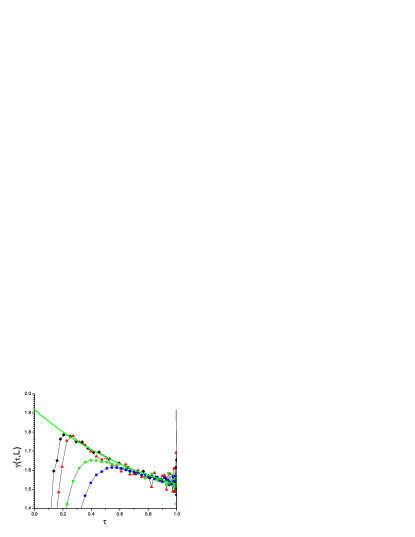
Figure 20: (Color online) The effective exponent $\gamma(\tau)$ Eqn. (22) for the bimodal $5$d ISG samples with $L=4,5,6,8$ (size coding as in Fig. 1), assuming $\beta_{c}=0.3925$. The extrapolation to $\tau=0$ gives $\gamma=1.92(5)$.

Luckily, according to daboul:04 for the systems studied $\theta$ is of the order of or a little greater than $1$, so the leading and subleading corrections have about the same exponent. An adequate analysis can be made using a joint effective correction term with a single effective $\theta$. Then extrapolation to criticality at $\tau=0$ can be made by first estimating the parameters $\gamma_{c}$ from the plot of $\gamma_{\mathrm{eff}}(\tau)$, Eqn. (25). Then, with fixed $\beta_{c}$ and $\gamma(0)$ the scaled spin glass susceptibility can be plotted in the form $\chi(\tau)\tau^{\gamma}$ against $\tau^{\theta}$ , Eqn. (26), with the correction to scaling exponent $\theta$ chosen such that the plot is a straight line over the thermodynamic limit data region. The parameters $C_{\chi}$ and $a_{\chi}$ can be read off this plot. All the parameters are adjusted until the fits to both equations (26) and (25) are optimised for the thermodynamic limit data. In practice the fits lead to accurately determined values for $\gamma_{c}$ and the other parameters, see e.g. Fig. 20. This value is fully reliable under the unique condition that $\beta_{c}$ has been correctly determined. An accurate knowledge of $\beta_{c}$ is essential; there is a one-to-one relationship between the estimate for the critical $\gamma(0)$ and the value of $\beta_{c}$ taken to construct the plot.

It can be noted that in the thermodynamic limit regime $L>\xi(\tau)$ there is ”self-averaging”, or in other words all individual ISG samples of a system have the same properties and in particular the same spin glass susceptibility. Thus in this regime there is no real need to average over large numbers of samples to obtain accurate measurements of the mean $\chi(\tau)$. In addition, equilibration in the thermodynamic limit region is relatively rapid so measurements are very reliable and not subject to equilibration difficulties. On the contrary, in the regime near, at and beyond $\beta_{c}$ ”lack of self-averaging” sets in; the inter-sample variability is important. The non-self-averaging parameters are size independent hukushima:00 ; palassini:03 at and beyond $\beta_{c}$ so however large the individual ISG samples they are all different from each other; there is a wide distribution of values of the spin glass susceptibility and other properties. The onset of a non-zero variability is a spin glass criterion for an approach to the transition temperature which obviously has no equivalent in pure systems such as simple ferromagnets. Even in diluted ferromagnets the non-self-averaging is non-zero in the thermodynamic limit only at $\beta=\beta_{c}$.

V Numerical simulations

For equilibration and measurements we used standard heat bath updating (without parallel tempering) on randomly selected sites. The samples (usually $64$) started off at infinite temperature and was then gradually cooled before reaching their final designated temperature. For temperatures near $T_{c}$ this means that each sample went through at least $10^{7}$, sometimes $10^{8}$, sweeps before any measurements took place. Normally there were about 10 sweeps between measurements, depending on temperature, maintaining on average $L^{d}$ spin flips between each measurement. For each sample and temperature we collected between $10^{6}$ and $10^{7}$ measurements depending on lattice size. The test for equilibration was discussed above. It can be noted that a sample with $L=8$ in dimension $5$ corresponds to as many individual spins as a sample with $L=32$ in dimension $3$.

VI Bimodal ISG in dimension five

No detailed numerical simulation measurements have been reported before for ISGs in dimension five. However, the analysis of a $15$ term High Temperature Series Expansion (HTSE) calculation daboul:04 gave the estimate $\beta_{c}^{2}=0.154(3)$, i.e. $\beta_{c}=0.3925(35)$, with a critical exponent $\gamma=1.95(15)$, for the bimodal ISG in $5$d. We have re-analyzed the two series in an unorthodox but transparent manner, Appendix I, and obtain values for $\beta_{c}$ and $\gamma$ very close to the central values in the original HTSE analysis but with additional information as to the strength of the correction to scaling term in the two cases. It can be seen that the correction to scaling is strong in the $5$d bimodal case (and practically negligible in the $5$d Gaussian case).

Numerical data derived from the various $P(q)(\beta,L)$ and $Q(q_{\ell})(\beta,L)$ distributions, all taken in the same runs on the same sets of samples for each $L$, are shown in Figures 1 to 7. The error bars correspond to inter-sample variability for each particular parameter.

The spin overlap $P(q)$ based phenomenological couplings $P$ kurtosis Eqn. (5), $P_{W}$ Eqn. (9), and the skewness of the absolute $P$ distribution Eqn. (10) show very similar forms. Because of the strong dispersion of individual sample parameter values, crossing points derived from the present data with a modest number of samples scatter and cannot provide an accurate estimate for $\beta_{c}$. The data are broadly compatible with the central HTSE estimate but on their own do not provide anything like a critical test, which for these parameters would require averaging over a much larger number of samples.

With the present sets of of samples, the most useful spin overlap parameter is the kurtosis of the absolute value distribution, $P_{\mathrm{abskurt}}(\beta,L)$ Eqn. (11). It shows a strong dip for each $L$ in the region of the HTSE $\beta_{c}$ estimate. The center of the dip as a function of temperature can be estimated quite accurately for each $L$. When the central dip positions are plotted against $1/L$ and extrapolated to $1/L=0$, the data give an estimate $\beta_{c}=0.392(3)$. This is the most precise estimate obtained from the spin overlap distributions and is fully consistent with the HTSE central value.

The link overlap parameters $Q_{w}(\beta,L)$ and $\ln(Q_{\mathrm{var}}-1)(\beta,L)$ show much smaller inter-sample variability than the parameters based on spin overlap. By luck $\ln(Q_{\mathrm{var}}-1)(\beta,L)$ has negligible finite size correction to scaling for the $5$d bimodal case; the curves for different $L$ all intersect at the same $\beta_{\mathrm{cross}}(L,L^{{}^{\prime}})=0.392(1)$, which coincides with the central value for $\beta_{c}$ from the HTSE estimate $\beta_{c}=0.3925(35)$ daboul:04 . This result both validates the assumption that this link overlap parameter is a bona fide phenomenological coupling, and improves the precision on the value of the critical temperature. For $Q_{w}(\beta,L)$ there are weak finite size corrections to scaling, but the intersection points $\beta_{\mathrm{cross}}(L,L^{{}^{\prime}})$ as functions of $L^{{}^{\prime}}$ for fixed $L$ can be extrapolated to infinite $L^{{}^{\prime}}$ to obtain an estimate $\beta_{c}=0.392(3)$ which is again in agreement with the HTSE value. In addition the (negative) maximum in the derivative $\mathrm{d}Q_{w}(\beta,L)/\mathrm{d}\beta$ deepens with increasing $L$ and its position $\beta_{\mathrm{max}}(L)$ can with extrapolation also be used to estimate $\beta_{c}$. The intersection criterion and the maximum slope criterion conveniently bracket the critical $\beta_{c}$ more and more closely as the sizes are increased. From these $Q_{\mathrm{var}}$ and $Q_{w}$ numerical data alone one can thus derive a very precise estimate $\beta_{c}=0.392(1)$, entirely consistent with the HTSE central estimate. The $Q$ kurtosis $Q_{k}$ and $Q$ skewness $Q_{s}$ peak positions are subject to finite size corrections but are also consistent with this estimate for $\beta_{c}$.

Thus the $5$d bimodal ISG is a particularly favorable case to validate the assumption that the link overlap parameters show strictly critical forms in ISGs as they do in a ferromagnet lundow:12 .

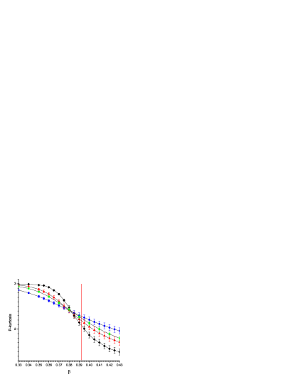
Figure 1: (Color online) The mean $P$ kurtosis Eqn. (5) for $5$d bimodal interaction samples with $L=4$ (blue circles), $L=5$ (green squares), $L=6$ (red triangles) and $L=8$ (black diamonds). The vertical red line corresponds to the HTSE $\beta_{c}$ central value daboul:04 .

Figure 2: (Color online) The mean $P_{W}$ parameter Eqn. (9) for the sets of $5$d bimodal interaction samples with $L=4,5,6,8$ (sizes coded as in Fig. 1). The vertical red line corresponds to the HTSE $\beta_{c}$ central value.

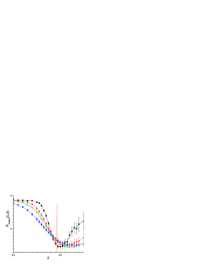
Figure 3: (Color online) The mean kurtosis of the absolute value spin overlap distribution, $P_{\mathrm{abskurt}}(\beta,L)$, Eqn. (11), for the sets of $5$d bimodal interaction samples $L=4,5,6,8$ (sizes coded as in Fig. 1). The vertical red line corresponds to the HTSE $\beta_{c}$ central value.

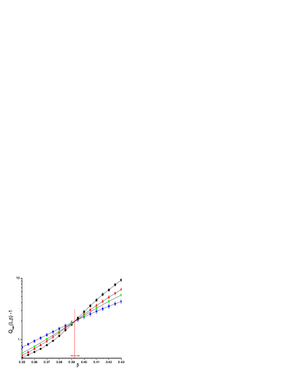
Figure 4: (Color online) The logarithm of the $Q$ variance Eqn. (15) minus $1$, $\ln(Q_{\mathrm{var}}-1)(\beta,L)$, for the sets of $5$d bimodal interaction samples with $L=4,5,6,8$ (sizes coded as in Fig. 1). The vertical red line corresponds to the HTSE $\beta_{c}$ central value. The horizontal red line represents the HTSE $\beta_{c}$ range daboul:04 .

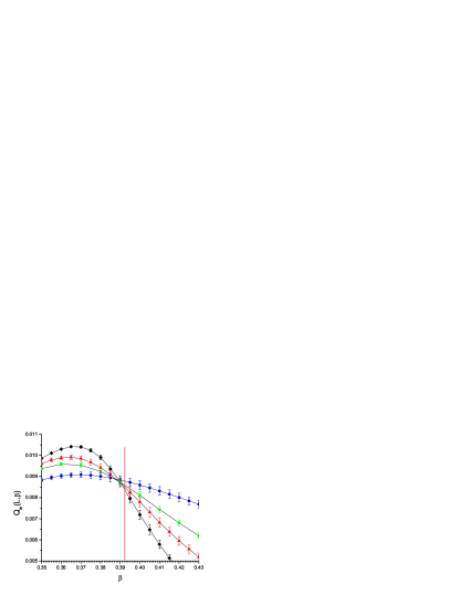
Figure 5: (Color online) The inverse normalized $Q$ variance $Q_{w}(\beta,L)$ Eqn. (18), for the sets of $5$d bimodal interaction samples with $L=4,5,6,8$ (sizes coded as in Fig. 1). The vertical red line corresponds to the HTSE $\beta_{c}$ central value.

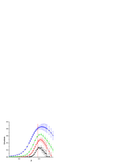
Figure 6: (Color online) The $Q$ kurtosis Eqn. (16), $Q_{k}(\beta,L)$, for the sets of $5$d bimodal interaction samples with $L=4,5,6,8$ (sizes coded as in Fig. 1). The vertical red line corresponds to the HTSE $\beta_{c}$ central value.

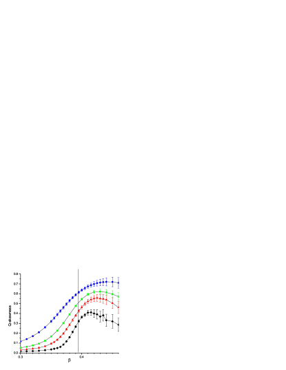
Figure 7: (Color online) The $Q$ skewness Eqn. (17), $Q_{s}(\beta,L)$, for the sets of $5$d bimodal interaction samples with $L=4,5,6,8$ (sizes coded as in Fig. 1). The vertical red line corresponds to the HTSE $\beta_{c}$ central value.

VII The Gaussian ISG in dimension 5

The critical temperature was estimated from the HTSE analysis to correspond to $\beta_{c}^{2}=0.174,0.176(3)$ or $0.177(3)$ according to the different analysis techniques daboul:04 , i.e. $\beta_{c}=0.420(3)$. The spin glass critical exponent was estimated by the HTSE analysis to be $\gamma=1.75(15)$.

The data for spin and link overlap moments and moment ratios are shown in Figs 8 to 11. The general form for each parameter is similar to that for the $5$d bimodal ISG, with the appropriate $\beta_{c}=0.421(2)$ being estimated from the absolute P kurtosis and from $Q_{w}$ allowing for corrections to scaling, in agreement with the central value from the HTSE analysis.

In the data for for the $Q$ kurtosis and the $Q$ skewness, Fig. 10 and Fig. 11, the peak positions are tending towards $\beta_{c}$ with increasing $L$ more slowly than in the bimodal case. This may be due to strong finite size corrections or possibly a peculiarity of the Gaussian interaction distribution.

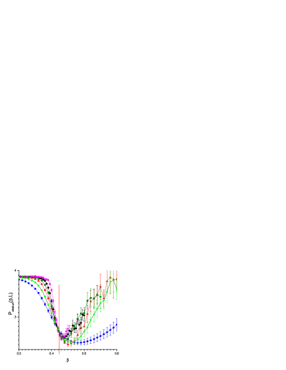
Figure 8: (Color online) The $P_{\mathrm{abskurt}}(\beta,L)$, Eqn. (11), for the sets of $5$d Gaussian interaction samples with $L=4,5,6,7,8,10$ (blue circles, green inverted triangles, red triangles, olive squares, black diamonds, pink left triangles) . The vertical red line corresponds to the HTSE central value $\beta_{c}=0.421$.

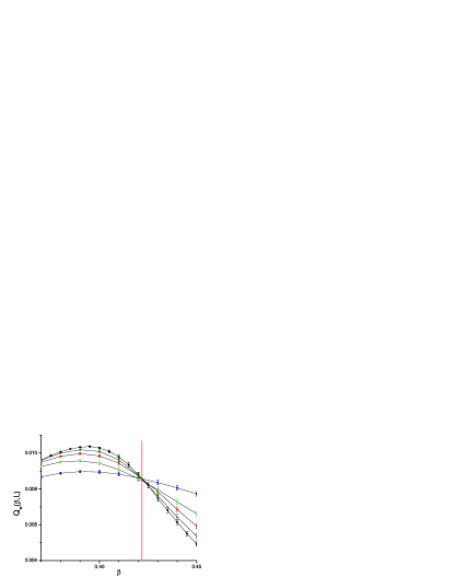
Figure 9: (Color online) The $Q_{w}(\beta,L)$ parameter of Eqn. (18), for the sets of $5$d Gaussian interaction samples with $L=4,5,6,7,8$ (sizes coded as in Fig. 8). The vertical red line corresponds to the HTSE central value $\beta_{c}=0.421$.

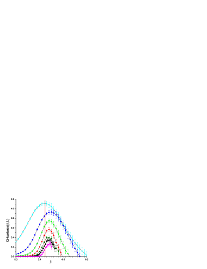
Figure 10: (Color online) The $Q$ kurtosis $Q_{k}(\beta,L)$ Eqn. (16), for the sets of $5$d Gaussian interaction samples with $L=3,4,5,6,7,8,10$ (sizes coded as in Fig. 8). The vertical red line corresponds to the HTSE central value$\beta_{c}=0.421$.

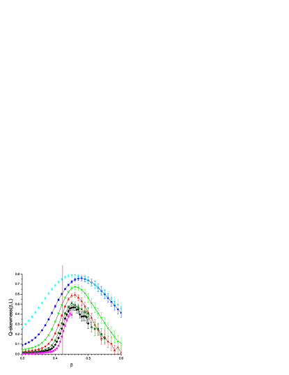
Figure 11: (Color online) The $Q$ skewness $Q_{s}(\beta,L)$ Eqn. (17), for the sets of $5$d Gaussian interaction samples with $L=3,4,5,6,7,8,10$ (cyan stars, blue circles, green inverted triangles, red triangles, olive squares, black diamonds, pink left triangles) . The vertical red line corresponds to the HTSE central value $\beta_{c}=0.421$.

VIII The bimodal ISG in dimension 4

From an analysis of HTSE data for the $4$d bimodal ISG, Daboul et al daboul:04 estimate $\beta_{c}^{2}=0.26(2)$, i.e. $\beta_{c}=0.51(2)$. (HTSE estimates in $4$d are intrinsically less precise than in $5$d). A critical temperature $\beta_{c}=0.493(7)$ was estimated marinari:99 from simulation measurements of high statistical accuracy to $L=10$ using the Binder parameter crossing point criterion, but corrections to scaling were not allowed for. A further estimate is $\beta_{c}=0.5025(25)$ bernardi:97 from unpublished Binder parameter data to $L=12$ by A.P. Young. From extensive domain wall free energy measurements to $L=10$ Hukushima gives an estimate $T_{c}=2.00(4)$ hukushima:99 , i.e. $\beta_{c}=0.50(1)$. In fact the raw data show significant finite size corrections, which affect the extrapolated estimate for the value of $\beta_{c}$ in the infinite size limit. This can be seen clearly in the data shown in Fig. $4$ of Ref. hukushima:99 ; the crossing points $T_{\mathrm{cross}}(L,L^{{}^{\prime}})$ evolve regularly from the smallest sizes to the largest sizes measured : $T_{\mathrm{cross}}(4,6)\sim 2.20,T_{\mathrm{cross}}(6,8)\sim 2.06,T_{\mathrm{cross}}(8,10)\sim 2.00$. By inspection, the infinite size limit crossing temperature must be distinctly lower than $T=2.00$, i.e. $\beta_{c}>0.50$ hukushima .

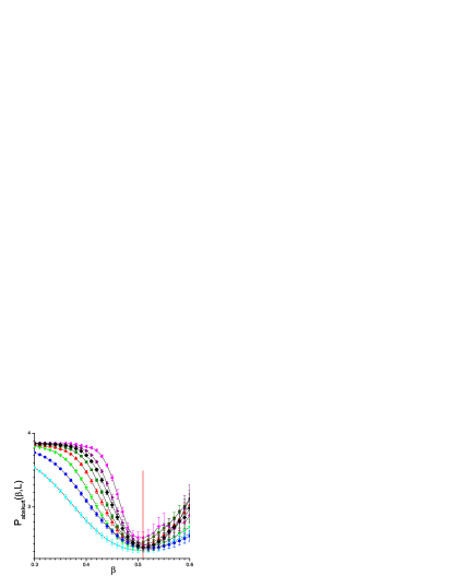
Figure 12: (Color online) The absolute $P$ kurtosis $P_{\mathrm{abskurt}}(\beta,L)$, Eqn. (11), for the sets of $4$d bimodal interaction samples with $L=3,4,5,6,7,8,9,12$ (cyan stars, blue circles, green inverted triangles, red triangles, olive squares, black diamonds, purple right triangles, pink left triangles). The vertical red line corresponds to the HTSE central value $\beta_{c}=0.51$

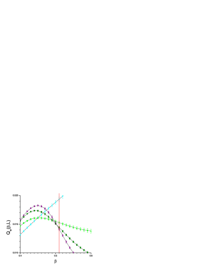
Figure 13: (Color online) The parameter $Q_{w}(\beta,L)$, Eqn. (18), for odd $L$ sets of $4$d bimodal interaction samples with $L=3,5,7,9$ (size coding as in Fig. 12). The vertical red line corresponds to the HTSE central value $\beta_{c}=0.51$

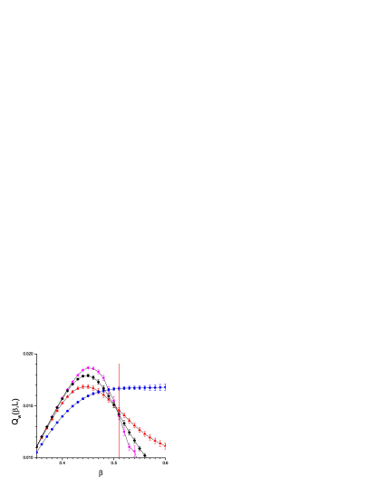
Figure 14: (Color online) The parameter $Q_{w}(\beta,L)$, Eqn. (18), for even $L$ sets of $4$d bimodal interaction samples with $L=4,6,8,12$ (size coding as in Fig. 12). The vertical red line corresponds to the HTSE central value $\beta_{c}=0.51$

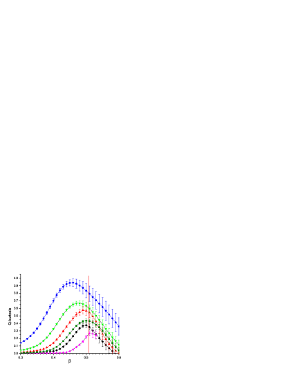
Figure 15: (Color online) The $Q$ kurtosis $Q_{k}(\beta,L)$, Eqn. (16), for sets of $4$d bimodal interaction samples with $L=4,5,6,7,8$ and $12$ (size coding as in Fig. 12). The vertical red line corresponds to the HTSE central value $\beta_{c}=0.51$

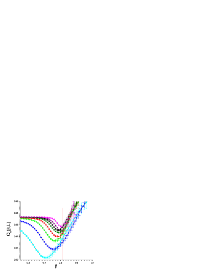
Figure 16: (Color online) The $Q$ deviation ratio $Q_{v}(\beta,L)$, Eqn. (19), for sets of $4$d bimodal interaction samples with $L=3,4,5,6,7,8,9$ and $12$ (size coding as in Fig. 12). The vertical red line corresponds to the HTSE central value $\beta_{c}=0.51$.

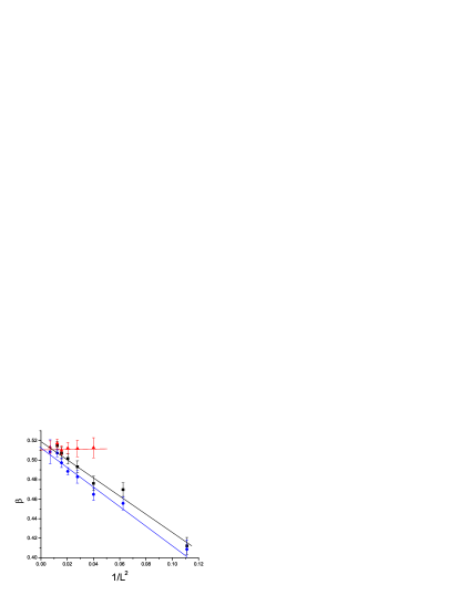
Figure 17: (Color online) The $Q$ kurtosis $Q_{k}(\beta,L)$ peak temperature $\beta_{\mathrm{max}}(L)$ (black squares), the $Q_{v}$ minimum location (blue circles) and the $\mathrm{d}Q_{w}/\mathrm{d}\beta$ minimum location (red triangles) against $1/L^{2}$ for sets of $4$d bimodal interaction samples with $L=3,4,5,6,7,8,9$. See Figs. 13, 14, 15 and 16 (derivative). The extrapolation to infinite $L$ gives $\beta_{c}=0.510(5)$. Error bars were obtained from statistical resampling of half the data set.

Simulations were carried out on sets of $64$ samples of size $L=3,4,5,6,7,8,9$ and $12$. As in $5$d the phenomenological couplings based on the spin overlap were strongly affected by the inter-sample variability; much larger sets would have been needed to obtain crossing point data for these parameters of similar statistical precision as in the earlier results for the Binder parameter. However, the position of $\beta_{\mathrm{dip}}$, the minimum of the dip in $P_{\mathrm{abskurt}}$, Fig 12, is independent of $L$ at $\beta_{\mathrm{dip}}=0.506(3)$ to within the statistical precision.

For the link overlap parameter $Q_{w}(\beta,L)$, Fig. 13 and Fig. 14, the inter-sample variability is much weaker than for the spin overlap phenomenological coupling parameters, so the crossing points for successive $L$ are better determined, but there are both finite size corrections with the crossing points evolving towards larger $\beta_{\mathrm{cross}}(L,L^{{}^{\prime}})$ with increasing $L,L^{{}^{\prime}}$, and odd-even effects in $L$.

Extrapolating to $1/L=0$ the $\beta_{\mathrm{cross}}(L−1,L+1)$ values for crossing points between $Q_{w}(\beta,L−1)$ and $Q_{w}(\beta,L+1)$ in Figs. 13 and 14 leads to the estimate $\beta_{c}=0.515(5)$ from this criterion. The deviation ratio $Q_{v}$, Fig. 16, also shows weak sample variability with a distinct minimum approaching $\beta_{c}$. The $Q$ kurtosis $Q_{k}(\beta,L)$, Fig. 15, and $Q$ skewness $Q_{s}(\beta,L)$ peak positions evolve with increasing $L$ towards limiting $\beta$ values for $1/L=0$ which are consistent with the estimate from $dQ_{w}/d\beta$, Fig. 17. It can be concluded that $\beta_{c}=0.510(5)$ in full agreement with the central HTSE estimate daboul:04 and with the previous numerical measurements once finite size corrections are fully allowed for.

IX The Gaussian ISG in dimension 4

High precision simulation measurements have been published for the $4$d Gaussian ISG, and for a $4$d diluted bimodal ISG jorg:08 . The critical temperature for the $4$d Gaussian ISG was estimated from Binder parameter and correlation length ratio measurements to be $\beta_{c}=0.554(3)$ in full agreement with earlier simulation estimates $0.555(3)$ parisi:96 ; ney:98 and with the HTSE estimate $\beta_{c}^{2}=0.314(4)$, i.e. $\beta_{c}=0.560(3)$.

Link overlap data for the parameter $Q_{w}$ measured for $64$ samples at each size are shown in Fig. 18 and 19. It can be seen that there are systematic finite size effects for the positions of the intersections between curves for different $L$, but these corrections have already become almost negligible by the largest sizes studied here as can be seen in Fig. 19. Even with the modest number of samples in these simulations, the link overlap $Q_{w}$ data provide an accurate independent estimate $\beta_{c}=0.554(2)$ which confirms the value of Ref. jorg:08 .

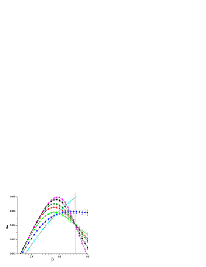
Figure 18: (Color online) The link overlap parameter $Q_{w}(\beta,L)$ for the $4$d Gaussian, $L=3,4,5,6,7,8,10$ (size coding as in Fig. 12)

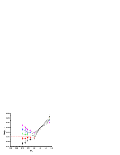
Figure 19: (Color online) The link overlap parameter $Q_{w}(\beta,L)$ for the $4$d Gaussian against $1/L$ for fixed $\beta$. Pink diamonds, blue inverted triangles, green triangles, red circles, black squares for $\beta=0.53,0.54,0.55,0.56,0.57$. The horizontal dashed line indicates the critical behavior in the large $L$ limit.

X The critical exponent $\gamma$

Daboul et al daboul:04 concluded that in each dimension the HTSE critical bimodal and Gaussian $\gamma$ values for the different interaction distributions which they studied were compatible with universality in ISGs to within the uncertainties of the HTSE analysis. However, their error bars for each $\gamma$ value were relatively large, as they did not have access to simulation data which supplement the HTSE calculations and which refine both the $\beta_{c}$ and the $\gamma$ estimates.

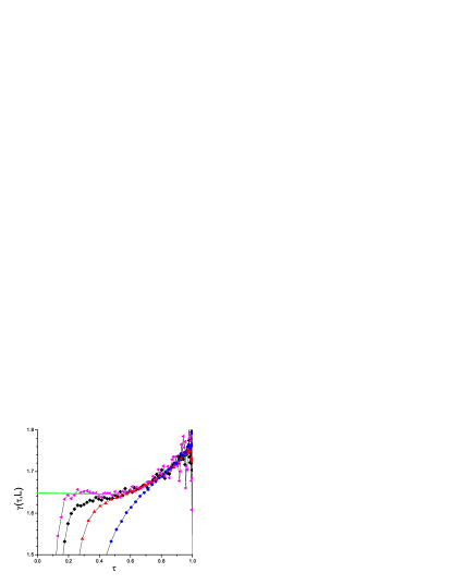
Figure 21: (Color online) The effective exponent $\gamma(\tau)$ Eqn. (22) for Gaussian $5$d ISG samples with $L=4,6,8,10$ (size coding as in Fig. 8), assuming $\beta_{c}=0.421$. The extrapolation to $\tau=0$ gives $\gamma=1.66(3)$.

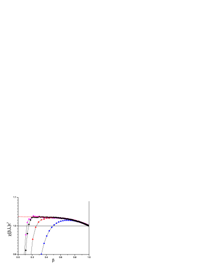
Figure 23: (Color online) The reduced susceptibility $\chi(\tau)\tau^{\gamma}$ for the Gaussian $5$d ISG samples $L=4,6,8,10$ (size coding as in Fig. 8), assuming $\beta_{c}=0.421$, $\gamma=1.66$. The overall thermodynamic limit fit is $\chi(\tau)=1.03\tau^{-1.66}[1+\cdots]$.

The effective $\gamma(\tau,L)$ values are defined by Eqn. (22), see the ”Critical exponent estimates” section. For the $5$d bimodal and $5$d Gaussian systems $\gamma(\tau,L)$ is shown in Fig. 20 and Fig. 21, with in each case $\tau=1-(\beta/\beta_{c})^{2}$, the data being plotted using the optimal values $\beta_{c}(\mathrm{bimodal})=0.392$ and $\beta_{c}(\mathrm{Gaussian})=0.421$ as quoted above. See also Figs. 22 and 23 for a plots of the reduced susceptibility in these cases with the assumed values of $\beta_{c}$ and critical exponents.

It can be noted that in $5$d a sample with $L=8$ is ”large” in the sense that for this size $\chi(\tau,L)$ remains in the thermodynamic limit until $\tau\sim 0.2$. To approach $\beta/\beta_{c}=1$ equally closely in $3$d would require samples with $L\sim 100$. The difference is a consequence of the much higher value of the exponent $\nu$ in dimension $3$, which is not far from the lower critical dimension where $\nu$ diverges.

For the $5$d bimodal ISG the plot of the effective $\gamma(\tau)$ shows a critical limit for the extrapolated thermodynamic limit regime $\gamma(0)=1.92(5)$, and a strong correction to scaling with exponent $\theta\sim 1$. With this value of $\gamma$ in hand $\chi(\tau)\tau^{\gamma}$ can be plotted as a function of $\tau$, Fig. 22, which can be fitted by $\chi(\tau)\tau^{\gamma}=0.59(1+0.69\tau)$. So finally for the $5$d bimodal ISG, in Eqn. (20) $\gamma=1.92(5),\theta\sim 1,C_{\chi}=0.59,a_{\chi}=0.69$. As $\theta\sim 1$ the second correction term in Eqn. (20) cannot be distinguished from the leading term. The fit curve for $\gamma_{\mathrm{eff}}(\tau)$ in Fig. 23 is the derivative of $\chi(\tau)$ with the same parameters. The parameter set including the sign and the approximate strength of $a_{\chi}$ are consistent with those which can be estimated entirely independently from the HTSE data (see Appendix I). The critical $\gamma$ and $\theta$ values are consistent with but more accurate than the HTSE value $\gamma=1.95(15)$ and $\theta\sim 1.1$ of Daboul et al daboul:04 .

For the $5$d Gaussian ISG the plot of the effective $\gamma(\tau)$ shows a critical limit $\gamma(0)=1.66(3),C_{\chi}=1.03$. The Daboul et al HTSE estimate is $\gamma=1.75(15)$. The correction to scaling is very weak except for a high order term in the region far from criticality, so no estimate can be made for $\theta$. Again the HTSE data, as analysed in Appendix I, are in complete agreement with all these conclusions : a very similar critical temperature, a very similar critical exponent, and the same weak correction to critical scaling.

The principal conclusion which can be drawn from the $5$d results, both from the simulations and from the HTSE data analyses, is that the critical exponent $\gamma=1.92(5)$ for the bimodal ISG is significantly higher than the critical $\gamma=1.66(3)$ for the Gaussian ISG.

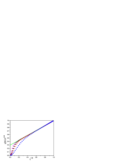
Figure 27: (Color online) The reduced susceptibility $\chi(\tau)\tau^{\gamma}$ for the bimodal $4$d ISG samples $L=4,6,8,12$ (size coding as in Fig. 12), assuming $\beta_{c}=0.51$, $\gamma=3.2$, $\theta=1.6$. The overall thermodynamic limit fit is $\chi(\tau)=0.30\tau^{-3.2}[1+2.3\tau^{1.6}]$.

The $4$d bimodal $\gamma(\tau)$ plots assuming $\beta_{c}=0.51$ are shown in Figs. 24 and 25. Extrapolating the thermodynamic limit regime curve to $\tau=0$ gives a critical exponent estimate $\gamma(0)=3.25(10)$ where the error bar corresponds principally to the residual uncertainty in $\beta_{c}$. The fit parameters to $\chi(\tau)\tau^{\gamma}$, Fig. 27, are $C_{\chi}=0.30$, $a_{\chi}=2.3$ and $\theta\sim 1.6$, so there is a very strong correction to scaling.

The estimate quoted from the HTSE analysis daboul:04 was $\gamma=2.5(3)$, for the same central value of $\beta_{c}$ as in the present work. We do not understand this. The raw HTSE susceptibility data are in excellent agreement with the numerical data (as they should be) and show a $\gamma_{\mathrm{eff}}(\tau)$ which is increasing rapidly as criticality is approached; $\gamma_{\mathrm{eff}}(\tau)$ is already greater than $2.5$ by $\tau=0.5$.

A re-analysis of unpublished $4$d bimodal $\chi(\beta)$ and $\xi(\beta)$ data of Ref. hukushima , are in full agreement with the present data as far as $\chi(\beta)$ is concerned. Fixing $\beta_{c}=0.51$ and defining $\nu_{\mathrm{eff}}(\tau)=\mathrm{d}\ln(\xi(\tau)/\beta)/\mathrm{d}\ln(\tau)$ campbell:06 , leads to an estimate for the correlation length critical exponent $\nu=1.30(5)$.

High precision simulation measurements have been made of the $4$d Gaussian ISG and of a $4$d diluted bimodal ISG jorg:08 . The critical temperature for the $4$d Gaussian ISG was estimated from Binder parameter and correlation length ratio measurements to be $\beta_{c}=0.554(3)$ in full agreement with earlier simulation estimates $0.555(3)$ parisi:96 ; ney:98 and with the HTSE estimate $\beta_{c}^{2}=0.314(4)$ i.e. $\beta_{c}=0.560(3)$.

For the Gaussian and the diluted bimodal ISG jorg:08 the critical exponents were estimated to be $\eta=-0.275(25)$ and $\nu=1.02(2)$ so $\gamma=(2-\eta)\nu=2.32(8)$, and $\eta=-0.275(25),\nu=1.025(15)$ so $\gamma=2.33(6)$ respectively. The simulation data showed that critical finite size corrections to scaling are weak. This is consistent with the criterion for $a_{\chi}$ given above. With the Gaussian critical parameters : $a_{\chi}\sim\gamma-z\beta_{c}^{2}=2.32(8)-2.45(2)=-0.13(10)$; the Wegner susceptibility correction to scaling amplitude will be small. Simulation and HTSE data for $\gamma_{\mathrm{eff}}(\tau)$ assuming $\beta_{c}=0.554$ are shown in Fig. 26; it can be seen that the corrections to scaling are indeed small, and by extrapolation to $\tau=0$ we find a critical $\gamma=2.35(2)$ in full agreement with Ref. jorg:08 . This can taken as a validation of the methodology used in the present work.

Naturally it was concluded in Ref. jorg:08 that as diluted bimodal and Gaussian $4$d ISGs have the same critical exponents to within the statistical uncertainties, universality is confirmed. However, the critical $\gamma=3.25(10)$ estimated above for the undiluted $4$d bimodal ISG is significantly higher than the $\gamma\sim 2.33$ values estimated for the Gaussian and the diluted bimodal ISGs. It happens that at the particular diluted bimodal bond concentration studied in Ref. jorg:08 , $p=0.35$, the kurtosis of the bond distribution is $1/0.35$, so almost exactly equal to the Gaussian distribution kurtosis which is $3$. It is tempting to speculate that there could be a universality rule for ISGs such that at fixed dimension, the exponents depend on the kurtosis of the interaction distribution, just as the critical temperature of an ISG in each dimension is a function of the kurtosis of the interaction distribution campbell:05 . For the moment we have not studied the ISGs in dimension $3$.

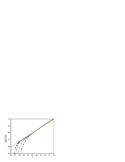
Figure 22: (Color online) The reduced susceptibility $\chi(\tau)\tau^{\gamma}$ for the bimodal $5$d ISG samples $L=4,5,6,8$ (size coding as in Fig. 8), assuming $\beta_{c}=0.3925$, $\gamma=1.92$. The overall thermodynamic limit fit is $\chi(\tau)=0.59\tau^{-1.92}[1+0.69\tau]$.

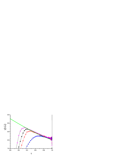
Figure 24: (Color online) The effective exponent $\gamma(\tau)$ Eqn. (22) for the bimodal $4$d ISG samples with $L=4,6,8,12$ (size coding as in Fig. 12), assuming $\beta_{c}=0.51$. The extrapolation to $\tau=0$ gives $\gamma=3.2(1)$

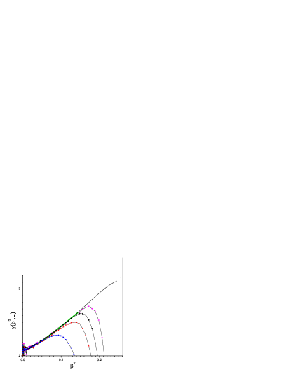
Figure 25: (Color online) The effective $\gamma(\beta^{2},L)$ presented in a different way for the bimodal $4$d ISG, assuming the HTSE critical temperature squared $\beta_{c}^{2}=0.26$. The simulation data $L=4,6,8,12$ have the same color coding as in Fig. 12. The thick green curve shows the explicitly summed HTSE data from the series given in daboul:04 . The thin black curve is the optimal polynomial fit to the thermodynamic limit regime data (series and numerical) extrapolated to $\beta_{c}^{2}$. The right hand side vertical line is at $\beta_{c}^{2}=0.26$.

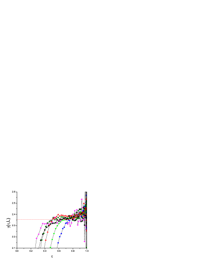
Figure 26: (Color online) The effective exponent $\gamma(\tau)$ Eqn. (22) for the Gaussian $4$d ISG samples with $L=4,5,6,7,8,10$ (size coding as in Fig. 12), assuming $\beta_{c}=0.554$. The extrapolation to $\tau=0$ gives $\gamma=2.35(2)$.The thick red curve shows the explicitly summed HTSE data from the series given in daboul:04 .

XI Conclusion

The moments and moment ratios of the link overlap distributions in ISGs show well defined critical properties, analogous to those observed for the link overlap distribution moments in a simple ferromagnet lundow:12 . The inter-sample variability of the link overlap parameters in the ISGs is weaker than that of the spin overlap parameters, so link overlap critical measurements, even with modest numbers of independent samples, are intrinsically more precise than spin overlap measurements. With larger numbers of samples, similar to those used in earlier simulation studies (e.g. Ref. jorg:08 ), and with negligible supplementary computational cost, extremely accurate $\beta_{c}$ values could be obtained from link overlap parameters.

Link overlap critical data have been used here to supplement spin overlap data and HTSE analyses in order to obtain accurate estimates for the ordering temperatures of ISGs in dimensions $4$ and $5$. We have also introduced a useful spin overlap dimensionless parameter, the absolute P distribution kurtosis $P_{\mathrm{abskurt}}$, Eqn. (11), which has not been previously studied. The $\beta_{c}$ values estimated from these simulations are all in excellent agreement with the entirely independent central estimates from HTSE analyses daboul:04 , but the estimates for the critical exponent $\gamma$ are more accurate. It should again be underlined that to obtain precise estimates of critical exponents it is essential to first establish reliable values for the critical temperatures. Once the ordering temperatures in hand, the effective critical exponents $\gamma(\tau)$ can be readily and reliably estimated from the appropriate derivative of the spin glass susceptibility simulation data, Eqn. (22), which can be extrapolated to $\tau=0$ to obtain $\gamma$.

The present critical $\gamma$ estimates – 5d bimodal $\gamma=1.92(5)$, 5d Gaussian $\gamma=1.66(3)$, 4d bimodal $\gamma=3.2(1)$, 4d Gaussian $\gamma=2.35(2)$ – can be compared with values obtained from analyses of the HTSE coefficients daboul:04 for both $5$d and $4$d, and compared with published simulation results jorg:08 for the $4$d Gaussian case. The simulation data show that both in $5$d and $4$d the critical $\gamma$ value for the bimodal ISG is significantly higher than the critical $\gamma$ values for the Gaussian ISG.

The well established universality rules which apply to standard second order transitions are that systems having the same spatial and spin dimensionalities all have identical critical exponents. From the present data it can be concluded empirically that different, more complicated, rules govern universality classes in Ising spin glasses. It should be remembered that ISG transitions are qualitatively very different from standard second order transitions. For an Ising ferromagnet in the regime below the Curie temperature there are just two mirror image families of spin up and spin down states. For an ISG the non-self-averaging behavior means that at and beyond $\beta_{c}$ even in the thermodynamic limit each individual sample has different properties, in particular a different spin overlap distribution and so a different spin glass susceptibility. It is not obvious that the powerful renormalization arguments which are so effective in standard transitions can be applied in the same manner in this context. It would be of interest to explore from fundamental principles which relevant parameters determine critical exponents in the spin glass family of transitions.

There are rare known cases of non-universality, such as the eight vertex model baxter:71 and the Ashkin-Teller model kadanoff:77 , which in the language of conformal invariance are all related to field theoretical models with central charge $c\geq 1$ (see e.g. sowinski:13 ). However, it is not clear to us if this is relevant to the ISG situation.

XII Acknowledgements

We are very grateful to K. Hukushima for comments and communication of unpublished data. The computations were performed on resources provided by the Swedish National Infrastructure for Computing (SNIC) at High Performance Computing Center North (HPC2N).

XIII Appendix

HTSE calculations in ISGs daboul:04 produce a set of terms for the spin glass susceptibility of the form

$$\chi(\beta^{2})=1+a_{1}\beta^{2}+a_{2}\beta^{4}+\cdots$$ (27)

Each coefficient $a_{i}$ is exact, but the series is in practice limited in length. The published ISG calculations have $15$ terms.

This series can be compared to the mathematical identity

$$(1-x)^{-\gamma}=1+\gamma x+\frac{\gamma(1+\gamma)}{2}x^{2}\\ +\frac{\gamma(1+\gamma)(2+\gamma)}{6}x^{3}+\cdots$$ (28)

for which the ratio of successive coefficients $a_{n}$ is

$$\frac{a_{n+1}}{a_{n}}=1+\frac{\gamma-1}{n+1}.$$ (29)

In the simplest case of a physical system with a critical spin glass susceptibility $\chi(\beta^{2})=C_{\chi}(1-\beta^{2}/\beta_{c}^{2})^{-\gamma}$, the ratio of successive terms $a_{n+1}/a_{n}$ in Eqn. (27) would be $(1/\beta_{c}^{2})(1+(\gamma-1)/(n+1))$. This suggests a graphical analysis in terms of a plot of this ratio against $1/(n+1)$, which is indeed a traditional technique for analyzing HTSE coefficients fisher:64 ; butera:02 . There are two complications. One is the Wegner confluent correction to scaling wegner:72 ; the critical susceptibility is

$$\chi(\tau)=C_{\chi}(\tau)^{-\gamma}\left(1+a_{\chi}\tau^{\theta}+\cdots\right)$$ (30)

where $\tau=1-\beta^{2}/\beta_{c}^{2}$. The ratios become (see butera:02 )

$$\frac{a_{n+1}}{a_{n}}=\frac{1}{\beta_{c}^{2}}\left(1+\frac{\gamma-1}{n+1}-\frac{a_{\chi}\theta\Gamma(\gamma)}{\Gamma(\gamma-\theta)(n+1)^{1+\theta}}\right)$$ (31)

so the initial slope is still $(\gamma-1)/\beta_{c}^{2}$ but there is a higher order term, which means that the plot of the ratio against $1/(n+1)$ becomes curved. This behavior is simply a reflection of the true temperature dependence of $\chi(\tau)$.

The second more annoying complication consists of series of ”parasitic” terms with alternating signs which arise from the presence of anti-ferromagnetic poles daboul:04 . Although when summed to infinite $n$ they give a zero or negligible contribution to the true susceptibility $\chi(\tau)$, in the ISG case they can lead to dramatic oscillations in the ratios $a_{n+1}/a_{n}$, Fig. 28 and Fig. 29. The series can nevertheless be analyzed, at least in dimension $4$d and above, using the Padé approximant technique, accompanied by methods known as $M1$ and $M2$ daboul:04 .

An unorthodox but transparent variant on the graphical method is the following. Suppose the initial series for $\chi(\beta)$ at some temperature $\beta<\beta_{c}$, terminating with term $n$, is written

$$\chi(n,x)=1+a_{1}x+a_{2}x^{2}+a_{3}x^{3}+\cdots+a_{n}x^{n}.$$ (32)

where $x=\beta^{2}$. Then terms can be regrouped

$$\chi^{*}(n+1,x)=1+\left(\frac{3a_{1}}{4}+\frac{a_{2}x}{4}\right)x\\ +\left(\frac{a_{1}}{4x}+\frac{a_{2}}{2}+\frac{a_{3}x}{4}\right)x^{2}\\ +\left(\frac{a_{2}}{4x}+\frac{a_{3}}{2}+\frac{a_{4}x}{4}\right)x^{3}+\cdots\\ +\left(\frac{a_{n}}{4x}+\frac{a_{n+1}}{2}+\frac{a_{n+2}x}{4}\right)x^{n+1}\\ =1+a^{*}_{1}x+\cdots+a^{*}_{n+1}x^{n+1}\\ =1+a_{1}x+\cdots+a_{n}x^{n}\\ +\frac{3a_{n+1}}{4}x^{n+1}+\frac{a_{n+2}}{4}x^{n+2}$$ (33)

The two sums $\chi(n,x)$ and $\chi^{*}(n+1,x)$ are identical up to the $n$th term. The series do not terminate in exactly the same place, but this is irrelevant as the aim is to extrapolate to infinite $n$ so as to obtain the true total $\chi(x)$. The essential point is that the sets of ratios of the successive coefficients $R^{*}(n+1)=a^{*}_{n+1}/a^{*}_{n}$ in the regrouped $\chi^{*}$ series now evolve smoothly with $1/(n+1)$, as can be seen in Figs. 30 and 31, and can be readily extrapolated to infinite $n$. This was certainly not the case for the raw series. The sum of the extrapolated regrouped terms can be considered a very good estimate of the true $\chi(x)$. It turns out that for the $5$d bimodal and Gaussian ISGs the set of regrouped term ratios are very insensitive to the choice of the trial $\beta^{2}$, and so the fit parameters for a representative $\beta^{2}$ provide good estimates for the true critical physical parameters. A simple fit $R^{*}(1/(n+1))=A+B(1/(n+1)+C(1/(n+1)^{2})$ provides estimates of the intercept $A=1/\beta_{c}^{2}$, the initial slope $B=(\gamma-1)/\beta_{c}^{2}$ and the strength of the Wegner correction to scaling $C=-a_{\chi}\theta\Gamma(\gamma)/(\Gamma(\gamma-\theta)\beta_{c}^{2})$ (For the fit we have assumed for convenience $\theta\sim 1$ daboul:04 but other values can be chosen for $\theta$ ). From Fig. 30, $\beta_{c}=0.3905,\gamma=1.85$ and $a_{\chi}\sim 2.0$ for the bimodal $5$d ISG, and from Fig. 31, $\beta_{c}=0.420,\gamma=1.68$ and $a_{\chi}\sim 0$ for the Gaussian $5$d ISG. The values of the critical temperatures and the critical exponents $\gamma$ are in excellent agreement with but appear to be more accurate than the central values from the much more sophisticated analysis of Daboul et al daboul:04 . In addition, this method provides an estimate of the strength of the Wegner correction term, which was not explicitly cited as a result of the analysis in Ref. daboul:04 .

It is important to underline that this technique is an analysis of the exact HTSE coefficients and so is entirely independent of the simulation data. Nevertheless the method again leads to a value for the bimodal critical exponent $\gamma\sim 1.85$ which is quite different from the Gaussian critical exponent $\gamma\sim 1.65$, in full agreement with the conclusions drawn from the simulation data.

In Ref.  daboul:04 the estimations of the critical exponents $\gamma$ in dimensions $7$ and $8$, above the upper critical dimension, are quoted as being greater than the exact theoretical value $\gamma=1$, which is suprising. The data can be reconciled with theory if there are strong correction terms. Thus the explicitly calculated $\chi(\tau)$ data points can be fitted by $\chi(\tau)=2.0\tau^{-1}[1-0.5\tau^{0.24}]$ in dimension $7$ and by $\chi(\tau)=1.6\tau^{-1}[1-0.375\tau^{0.30}]$ in dimension $8$. It can be remembered that there are corrections to scaling above the upper critical dimension in the pure ferromagnetic Ising model berche:08 .

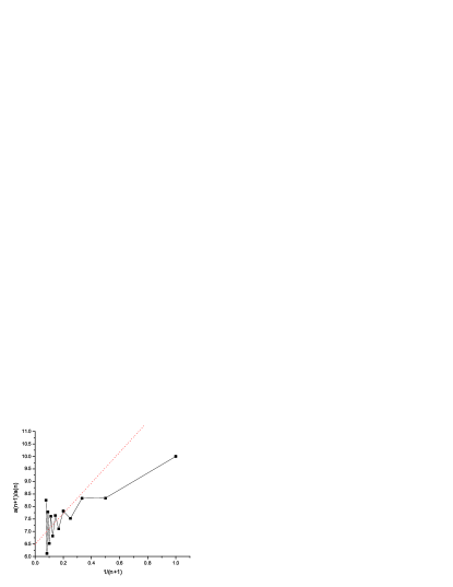
Figure 28: (Color online) The raw coefficient ratios $a(n+1)/a(n)$ in the HTSE susceptibility series for the bimodal ISG in dimension 5 ($a(n)$ data from daboul:04 ).

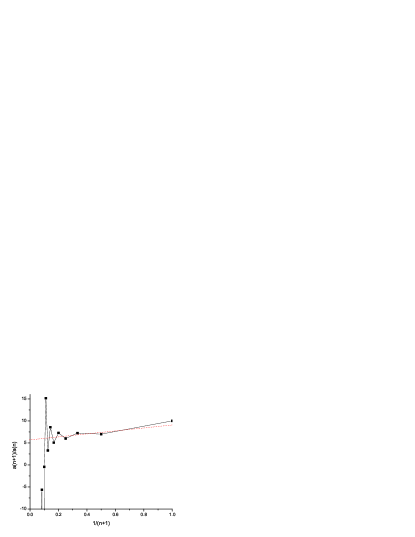
Figure 29: (Color online)The raw coefficient ratios $a(n+1)/a(n)$ in the HTSE susceptibility series for the Gaussian ISG in dimension 5 ($a(n)$ data from daboul:04 ).

Figure 30: (Color online) The regrouped coefficient ratios $a^{*}(n+1)/a^{*}(n)$ in the HTSE susceptibility series for the bimodal ISG in dimension 5 for $\beta^{2}=9$.

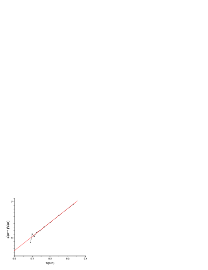
Figure 31: (Color online) The regrouped coefficient ratios $a^{*}(n+1)/a^{*}(n)$ in the HTSE susceptibility series for the Gaussian ISG in dimension 5 for $\beta^{2}=10$.

References

- (1) S. Caracciolo, G. Parisi, S. Patarnello, and N. Sourlas, J. Phys. (Paris) 51, 1877 (1990).
- (2) H. Bokil, B. Drossel, and M. A. Moore, Phys. Rev. B 62, 946 (2000).
- (3) P. Contucci, C. Giardina, C. Giberti, and C. Vernia, Phys. Rev. Lett. 96, 217204 (2006).
- (4) H.G. Katzgraber, M. K¨orner, and A. P. Young, Phys. Rev. B 73, 224432 (2006).
- (5) M. Hasenbusch, A. Pelissetto, and E. Vicari, Phys. Rev. B 78, 214205 (2008).
- (6) T. Jörg and H. G. Katzgraber, Phys.Rev.B 77, 214426 (2008).
- (7) D. Daboul, I. Chang and A. Aharony, Eur. Phys. J. B 41, 231 (2004).
- (8) L. W. Bernardi, S. Prakash, and I. A. Campbell, Phys. Rev. Lett. 77, 2798 (1996).
- (9) M. Henkel and M. Pleimling, Europhys. Lett. 69, 524 (2005).
- (10) I. A. Campbell and D. C. M. C. Petit, J. Phys. Soc. Japan, 79, 011006 (2010)
- (11) K. Hukushima and H. Kawamura, Phys. Rev. E 62, 3360 (2000).
- (12) M. Palassini, M. Sales and F. Ritort, Phys. Rev. B 68, 224430 (2003).
- (13) P.H. Lundow and I.A. Campbell, arXiv:1211.2006.
- (14) H. G. Katzgraber, M. Palassini, and A. P. Young, Phys. Rev. B, 63, 184422 (2001).
- (15) R. Alvarez Banos et al. (Janus Collaboration), J. Stat. Mech. 2010, P06026.
- (16) F. Wegner, Phys. Rev. B 5, 4529 (1972).
- (17) I. A. Campbell, K. Hukushima, and H. Takayama, Phys. Rev. Lett. 97, 117202 (2006).
- (18) P. Butera and M. Comi, Phys. Rev. B 65, 144431 (2002).
- (19) E. Marinari and F. Zuliani, J. Phys. A 32, 7447 (1999).
- (20) L. W. Bernardi and I. A. Campbell, Phys. Rev. B 56, 5271 (1997).
- (21) K. Hukushima, Phys. Rev. E 60, 3606 (1999).
- (22) K. Hukushima, private communication.
- (23) G. Parisi, F. Ricci-Tersenghi, and J. J. Ruiz-Lorenzo, J. Phys. A 29, 7943 (1996).
- (24) M. Ney-Nifle, Phys. Rev. B 57, 492 (1998).
- (25) I.A. Campbell, Phys. Rev. B 72, 092405 (2005).
- (26) R. Baxter, Phys. Rev. Lett. 26, 832 (1971)
- (27) L.P. Kadanoff, Phys. Rev. Lett. 39, 903 (1977)
- (28) T. Sowiński, R. W. Chhajlany, O. Dutta, L. Tagliacozzo and M. Lewenstein, arXiv:1304.4835
- (29) M. E. Fisher and D. S. Gaunt, Phys. Rev. A 133, 224 (1964).
- (30) B. Berche, C. Chatelain, C. Dhall, R. Kenna, R. Low, and J.-C.Walter, J. Stat. Mech. 2008, P11010.