Performance Evaluation of Sparse Matrix Multiplication Kernels on Intel Xeon Phi

Abstract

Intel Xeon Phi is a recently released high-performance coprocessor which features $61$ cores each supporting $4$ hardware threads with $512$-bit wide SIMD registers achieving a peak theoretical performance of 1Tflop/s in double precision. Many scientific applications involve operations on large sparse matrices such as linear solvers, eigensolver, and graph mining algorithms. The core of most of these applications involves the multiplication of a large, sparse matrix with a dense vector (SpMV). In this paper, we investigate the performance of the Xeon Phi coprocessor for SpMV. We first provide a comprehensive introduction to this new architecture and analyze its peak performance with a number of micro benchmarks. Although the design of a Xeon Phi core is not much different than those of the cores in modern processors, its large number of cores and hyperthreading capability allow many application to saturate the available memory bandwidth, which is not the case for many cutting-edge processors. Yet, our performance studies show that it is the memory latency not the bandwidth which creates a bottleneck for SpMV on this architecture. Finally, our experiments show that Xeon Phi’s sparse kernel performance is very promising and even better than that of cutting-edge general purpose processors and GPUs.

1 Introduction

Given a large, sparse, $m\times n$ matrix $\mathbf{A}$, an input vector $\mathbf{x}$, and a cutting edge shared-memory multi/many core architecture Intel Xeon$\textregistered$ Phi, we are interested in analyzing the performance obtained while computing

$$\mathbf{y}\leftarrow\mathbf{A}\mathbf{x}$$

in parallel. The computation, known as the sparse-matrix vector multiplication (SpMV), and some of its variants, such as the sparse-matrix matrix multiplication (SpMM), form the computational core of many applications involving linear systems, eigenvalues, and linear programs, i.e., most large scale scientific applications. For this reason, they have been extremely intriguing in the context of high performance computing (HPC). Efficient shared-memory parallelization of these kernels is a well studied area  [1, 2, 3, 9, 18], and there exist several techniques such as prefetching, loop transformations, vectorization, register, cache, TLB blocking, and NUMA optimization, which have been extensively investigated to optimize the performance [7, 11, 12, 18]. In addition, company-built support is available for many parallel shared-memory architectures, such as Intel’s MKL and NVIDIA’s cuSPARSE. Popular 3rd party sparse matrix libraries such as OSKI [17] and pOSKI [8] also exist.

Intel Xeon Phi is a new coprocessor with many cores, hardware threading capabilities, and wide vector registers. The novel architecture is of interest for HPC community: the Texas Advanced Computing Center has built the Stampede cluster which is equipped with Xeon Phi and many other computing centers are following. Furthermore, some effort has been pushed to have a fast MPI implementation [13]. Although Intel Xeon Phi has been released recently, performance evaluations already exist in literature [6, 15, 16]. Eisenlohr et al. investigated the behavior of dense linear algebra factorization on Xeon Phi [6] and Stock et al. proposed an automatic code optimization approach for tensor contraction kernels [16]. Both of these works work on dense and regular data. in a previous work, two of the authors evaluates the scalability of graph algorithms, coloring and breadth first search (BFS) [15]. None of these works give absolute performance values and to the best of our knowledge there exist no such work in the literature. Although similar to BFS, SpMV and SpMM are different kernels (in terms of synchronization, memory access, and load balancing), and as we will show, the new coprocessor is very promising and can even perform better than existing cutting-edge CPUs and accelerators while handling sparse linear algebra.

Accelerators/coprocessors are designed for specific tasks. They do not only achieve a good performance but also reduce the energy usage per computation. Up to now, GPUs have been successful w.r.t. these criteria and they reported to perform well especially for regular computations. However, the irregularity and sparsity of SpMV-like kernels create several problems for these architectures. In this paper, we analyze how Xeon Phi performs on two popular sparse linear algebra kernels, SpMV and SpMM. [4] studied the performance of a Conjugate Gradient application which uses SpMV, however this study concerns only a single matrix and is application oriented. To the best of our knowledge, we give the first analysis of the performance of the coprocessor on these kernels.

We conduct several experiments with 22 matrices from UFL Sparse Matrix Collection. To have architectural baselines, we also measured the performance of two dual Intel Xeon processors, X5680 (Westmere) E5-2670 (Sandy Bridge), and two NVIDIA Tesla$\textregistered$ GPUs C2050 and K20, on these matrices. Overall, Xeon Phi’s sparse matrix performance is very promising and even better than that of general purpose CPUs and the GPUs we used in our experiments. Furthermore, its large registers and extensive vector instruction support boost its performance and make it a candidate for both scientific computing and throughput oriented server-side code for SpMV/SpMM-based services such as product/friend recommendation.

Having 61 cores and hyperthreading capability can help the Intel Xeon Phi to saturate the memory bandwidth during SpMV, which is not the case for many cutting edge processors. Yet, our analysis showed that the memory latency, not the memory bandwidth, is the bottleneck and the reason for not reaching to the peak performance. As expected, we observed that the performance of the SpMV kernel highly depends on the nonzero pattern of the matrix and its sparsity: when the nonzeros in a row are aligned and packed in cachelines in the memory, the performance would be much better. We investigate two different approaches of densifying the computation either by ordering the matrix via the well known reverse Cuthill-McKee ordering RCM [5] or changing the nature of the computation by register blocking.

The paper is organized as follows: Section 2 presents a brief architectural overview of the Intel Xeon Phi coprocessor along with some detailed read and write memory bandwidth micro benchmarks. Section 3 describes the sparse-matrix multiplication kernels and Sections 4 and 5 analyze Xeon Phi’s performance on these kernels. The performance comparison against other cutting-edge architectures is given in Section 6. Section 7 concludes the paper.

2 The Intel Xeon Phi Coprocessor

In this work, we use a pre-release KNC card SE10P. The card has 8 memory controllers where each of them can execute 5.5 billion transactions per second and has two 32-bit channels. That is the architecture can achieve a total bandwidth of 352GB/s aggregated across all the memory controllers. There are 61 cores clocked at 1.05GHz. The cores’ memory interface are 32-bit wide with two channels and the total bandwidth is 8.4GB/s per core. Thus, the cores should be able to consume 512.4GB/s at most. However, the bandwidth between the cores and the memory controllers is limited by the ring network which connects them and theoretically supports at most 220GB/s.

Each core in the architecture has a 32kB L1 data cache, a 32kB L1 instruction cache, and a 512kB L2 cache. The architecture of a core is based on the Pentium architecture: though its design has been updated to 64-bit. A core can hold 4 hardware contexts at any time. And at each clock cycle, instructions from a single thread are executed. Due to the hardware constraints and to overlap latency, a core never executes two instructions from the same hardware context consecutively. In other words, if a program only uses one thread, half of the clock cycles are wasted. Since there are 4 hardware contexts available, the instructions from a single thread are executed in-order. As in the Pentium architecture, a core has two different concurrent instruction pipelines (called U-pipe and V-pipe) which allow the execution of two instructions per cycle. However, some instructions are not available on both pipelines: only one vector or floating point instruction can be executed at each cycle, but two ALU instructions can be executed in the same cycle.

Most of the performance of the architecture comes from the vector processing unit. Each of Intel Xeon Phi’s cores has 32$\times$512-bit SIMD registers which can be used for double or single precision, that is, either as a vector of 8$\times$64-bit values or as a vector of 16$\times$32-bit values, respectively. The vector processing unit can perform many basic instructions, such as addition or division, and mathematical operations, such as sine and sqrt, allowing to reach 8 double precision operations per cycle (16 single precision). The unit also supports Fused Multiply-Add (FMA) operations which are typically counted as two operations for benchmarking purposes. Therefore, the peak performance of the SE10P card is 1.0248 Tflop/s in double precision (2.0496 Tflop/s in single precision) and half without FMA.

2.1 Read-bandwidth benchmarks

We first try to estimate what is the maximum achievable read bandwidth in Xeon Phi. By benchmarking the performance on simple operations by different number of cores and threads per core, we can have an idea about where the performance bottlenecks come from. To that end, we choose the array sum kernel which just computes the sum of large arrays. And we measure the amount of effective (application) bandwidth reached. To compute the sum, each core first allocates 16MB of data and then each thread reads the whole data. To minimize cache reusage, each thread starts from a different array. All the results of this experiment are presented in Figure 1 where the aggregated bandwidth is reported for char and int data types.

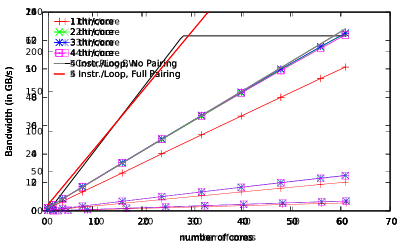
(a) Simple sum, char, -O1

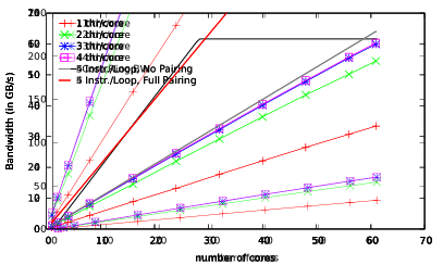
(b) Simple sum, int, -O1

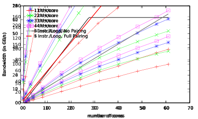
(c) Vectorization

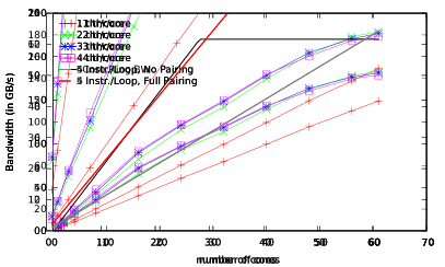
(d) Vectorization + prefetching

Figure 1: The read bandwidth obtained by Intel Xeon Phi on our micro-benchmarks containing different array sum operations. In (a) and (b), an upper bound on bandwidth is computed by the 1.05Ghz core speed where 4 instructions are required per int and 5 instructions (including an additional casting) is required per char. In (c) and (d), the theoretical upper bound on maximum bandwidth, $\max$(8.4GB/s $\times$ #cores, 220GB/s), due to maximum per core and ring bandwidths is shown.

First we sum the array as a set of 8-bit integers, i.e., char data type. The benchmark is compiled via -O1 optimization flag so as to prevent the compiler optimizations with possible undesired effects. The results are shown in Figure 1(a). The bandwidth peaks at 12GB/s when using 2 threads per core and 61 cores. The bandwidth scales linearly with the number of cores indicating that the benchmark does not saturate the memory bus. Moreover, additional threads per core do not bring significant performance improvements which indicates a full usage of the computational resources in the cores. To show that we have plotted peak effective bandwidth one can expect to achieve if instructions can utilize both pipelines (denoted as Full Pairing in the figure) or not (denoted as No Pairing). For this particular code, compiled executable have 5 instructions per loop. As seen in the figure, best achieved performance aligns well with No Pairing line, indicating that those 5 instructions were not paired, and this benchmark is instruction bound.

The second benchmark performs the summation on the arrays containing 32-bit ints. Again, we employ the -O1 optimization flag. The results are presented in Figure 1(b). This code has 4 instructions in the loop and process 4 times more data in each instruction, hence the performance is roughly scaled 5 times. The performance still scales linearly with the number of cores indicating the performance is not bounded by the speed of the memory interconnect. The peak bandwidth, 60.0GB/s, is achieved by using 4 threads per core. There is only a small difference with the bandwidth achieved using 3 threads (59.9GB/s), which implies that the benchmark is still instruction bound. Though we can notice that 2 threads were not enough to achieve peak bandwidth (54.4GB/s) and at least 3 threads are necessary to hide memory latency.

The third benchmark also considers the array as a set of 32-bit integers but uses vector operations to load and sum 16 of them at a time, i.e., it processes 512 bits, a full cacheline, at once. The results are presented in Figure 1(c). The bandwidth peaks at 171GB/s when 61 cores and 4 threads per core are used. This benchmark is more memory intensive than the previous ones, and even 3 threads per core can not hide memory latency. Moreover, although it is not very clear in the figure, the bandwidth scales sub-linearly with the increasing number of cores. This indicates the bandwidth is getting closer to the speed of the actual memory bus.

The fourth benchmark tries to improve on the previous one by removing the necessity of hiding the memory latency via using memory prefetching. The results are presented in Figure 1(d). The bandwidth peaks at 183GB/s when 61 cores and 2 threads per core are used (representing 3GB/s per core). The bandwidth with a single thread per core is relatively worse (149GB/s) and scales linearly with the number of cores. However, with 2 threads, the performance no longer scales linearly from 24 cores and seems to have almost plateaued at 61 cores. A single core can sustain 4.8GB/s of read bandwidth when it is alone accessing the memory.

2.2 Write-bandwidth benchmarks

After the read bandwidth, we also want to investigate how write bandwidth behaves with a set of micro benchmarks in which each thread allocates a local 16MB buffer and fills it with some predetermined value. The results are presented in Figure 2.

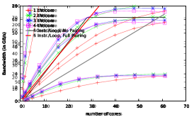
(a) Store

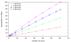
(b) Vectorization + No-Read hint

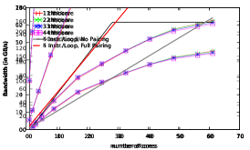
(c) Vectorization + No-Read hint + No global ordering

Figure 2: The write bandwidth obtained by Intel Xeon Phi on three micro-benchmarks using different approaches for memsetting the buffer. In (c), the theoretical upper bound on maximum bandwidth due to maximum per core and ring bandwidths is shown.

From the previous micro benchmarks on read bandwidth, it should be clear that non-vectorized loops will not perform well since they will be instruction bound, so we do not consider non-vectorized cases. The first benchmark uses fills the memory by crafting a buffer in a 512-bit SIMD register and writing a full cache line at once using the simple store instruction. As shown in Figure 2(a), when all 61 cores are used, a bandwidth of 65-70GB/s is achieved for each thread per core configuration. The second benchmark writes to memory using the No-Read hint. This bypasses the Read For Ownership protocol which forces to read a cacheline even before overwriting its whole content. Note that the protocol is important in case of partial cacheline updates. The results of that benchmark are presented in Figure 2(b). The achieved bandwidth scales linearly up to 100GB/s using 61 cores and 4 threads per core. It also improves linearly with the number of threads which indicates that the cores are stalling write operations.

The third benchmark uses a different instruction to perform the memory write. Regular write operations enforces that the writes are committed to the memory in the same order the instructions were emitted. This property is crucial to ensure the coherency in many shared memory parallel algorithms. The instruction used in this benchmark allow the writes to be Non-Globally Ordered. (This also uses the No-Read hint). The results of the benchmark are presented in Figure 2(c). With this instruction, the 100GB/s bandwidth obtained in the previous experiment is achieved with only 24 cores. The bandwidth peaks at 160GB/s when all 61 cores are used (representing 2.6GB/s per core). Note that it can be achieved by using a single thread per core. This instruction allows not to stall the threads until the internal buffer of the architecture is full, and a single thread can manage to fill it up.A single core can sustain 5.6GB/s of write bandwidth when it is alone accessing the memory.

3 Sparse Multiplication Kernels

The most well-known sparse-matrix kernel is in the form $\mathbf{y}\leftarrow\mathbf{A}\mathbf{x}$ where $\mathbf{A}$ is an $m\times n$ sparse matrix, and $\mathbf{x}$ and $\mathbf{y}$ are $n\times 1$ and $m\times 1$ column vectors (SpMV). In this kernel, each nonzero is accessed, multiplied with an $\mathbf{x}$-vector entry, and the result is added to a $\mathbf{y}$-vector entry once. That is, there are two reads and one read-and-write per each nonzero accessed. Another widely-used sparse multiplication kernel is the sparse matrix-dense matrix multiplication (SpMM) in which $\mathbf{x}$ and $\mathbf{y}$ are $n\times k$ and $m\times k$ dense matrices. In SpMM, there are $k$ reads and $k$ read-and-writes per each nonzero accessed. The read and write access patterns of these kernels are given in Figure 3(a). Obtaining good performance for SpMV is difficult almost on any architecture. The difficulty arises from the sparsity pattern of $\mathbf{A}$ which yields a non-regular access to the memory. The amount of computation per nonzero is also very small. Most of the operations suffer from bandwidth limitation.

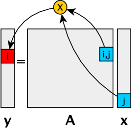
(a) SpMV

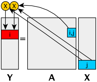
(b) SpMM

Figure 3: Memory access patterns for SpMV and SpMM. The color blue shows reads and red shows writes.

An $m\times n$ sparse matrix $\mathbf{A}$ with $\tau$ nonzeros is usually stored in the compressed row (or column) storage format CRS (or CCS). Two formats are dual of each other. Throughout the paper, we will use CRS hence, we will describe it here. CRS uses three arrays:

• cids[.] is an integer array of size $\tau$ that stores the column ids for each nonzero in row-major ordering.

• rptrs[.] is an integer array of size $m+1$. For $0\leq i<m$, rptrs[i] is the location of the first nonzero of $i$th row in the cids array. The first element is rptrs[0] $=0$, and the last element is rptrs[m] $=\tau$. Hence, all the column indices of row $i$ is stored between cids[rptrs[i]] and ${\it cids}[{\it rptrs}[i+1]]-1$.

• val[.] is an array of size $\tau$. For $0\leq i<\tau$, val[i] keeps the value corresponding to the nonzero in cids[i].

There exist other sparse matrix representations [14], and the best storage format almost always depends on the pattern of the matrix and the kernel. In this work, we use CRS as it constitutes a solid baseline. Since $\mathbf{A}$ is represented in CRS, it is a straightforward task to assign a row to a single thread in a parallel execution. As Figure 3(a) shows, each entry $\mathbf{y}_{i}$ of the output vector can be computed independently while streaming the matrix row by row. While processing a row $i$, multiple $\mathbf{x}$ values are read, and the sum of the multiplications is written to $\mathbf{y}_{i}$. Hence, there are one multiply and one add operation per nonzero, and the total number of floating point operations is $2\tau$.

4 SpMV on Intel Xeon Phi

For the experiments, we use a set of $22$ matrices in total whose properties are given in Table 1. The matrices we are taken from the UFL Sparse Matrix Collection with one exception mesh_2048 which corresponds to a 5-point stencil mesh in 2D with size $2048\times 2048$. We store the matrices in memory by using the CRS representation. All scalar values are stored in double precision (64-bit floating point). And all the indices are stored via $32$-bit integers. For all the experiments and figures in this section, the matrices are numbered from $1$ to $22$ by increasing number of nonzero entries, as listed in the table. For all the experiments, we first run the operation 70 times and compute the averages of the last 60 operations which are shown in figures and tables. Caches are flushed between each measurement.

Table 1: Properties of the matrices used in the experiments. All matrices are square.

						max	max
#	name	#row	#nonzero	density	nnz/row	nnz/r	nnz/c
1	shallow_water1	81,920	204,800	3.05e-05	2.50	4	4
2	2cubes_sphere	101,492	874,378	8.48e-05	8.61	24	29
3	scircuit	170,998	958,936	3.27e-05	5.60	353	353
4	mac_econ	206,500	1,273,389	2.98e-05	6.16	44	47
5	cop20k_A	121,192	1,362,087	9.27e-05	11.23	24	75
6	cant	62,451	2,034,917	5.21e-04	32.58	40	40
7	pdb1HYS	36,417	2,190,591	1.65e-03	60.15	184	162
8	webbase-1M	1,000,005	3,105,536	3.10e-06	3.10	4700	28685
9	hood	220,542	5,057,982	1.03e-04	22.93	51	77
10	bmw3_2	227,362	5,757,996	1.11e-04	25.32	204	327
11	pre2	659,033	5,834,044	1.34e-05	8.85	627	745
12	pwtk	217,918	5,871,175	1.23e-04	26.94	180	90
13	crankseg_2	63,838	7,106,348	1.74e-03	111.31	297	3423
14	torso1	116,158	8,516,500	6.31e-04	73.31	3263	1224
15	atmosmodd	1,270,432	8,814,880	5.46e-06	6.93	7	7
16	msdoor	415,863	9,794,513	5.66e-05	23.55	57	77
17	F1	343,791	13,590,452	1.14e-04	39.53	306	378
18	nd24k	72,000	14,393,817	2.77e-03	199.91	481	483
19	inline_1	503,712	18,659,941	7.35e-05	37.04	843	333
20	mesh_2048	4,194,304	20,963,328	1.19e-06	4.99	5	5
21	ldoor	952,203	21,723,010	2.39e-05	22.81	49	77
22	cage14	1,505,785	27,130,349	1.19e-05	18.01	41	41

4.1 Performance evaluation

The SpMV kernel is implemented in C++ using OpenMP and processes the rows in parallel. We tested our dataset with multiple scheduling policies. Figure 4 presents the highest performance obtained when compiled with -O1 and -O3. In most cases, the best performance is obtained either using 61 cores and 3 threads per core, or using 60 cores and 4 threads per core. The dynamic scheduling policy with a chunk size of 32 or 64 is typically giving the best results.

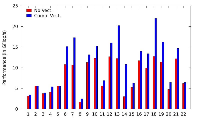
Figure 4: Comparing -O1 (No Vect.) and -O3 (Comp. Vect.) for SpMV in Xeon Phi.

When compiled with -O1, the performance obtained varies from $1$ to $13$GFlop/s. Notice that the difference of performance is not correlated to the size of the matrix. When compiled with -O3 the performance rises for all matrices and reaches 22GFlop/s on nd24k. In total, $5$ matrices from our set achieve a performance over 15GFlop/s.

An interesting observation is that the difference on performance is not constant; it depends on the matrix. Analyzing the assembly code generated by the compiler for the SpMV inner loop (which computes the dot product between a sparse row of the matrix and the dense input vector) gives an insight on why the performances differ. When -O1 is used, the dot product is implemented in a simple way: the column index of the nonzero is put in a register. And the value of the nonzero is put in another. Then, the nonzero is multiplied with the input vector element (it does not need to be brought to register, a memory indirection can be used here). The result is accumulated. The nonzero index is incremented and tested for looping purposes. In other words, the dot product is computed one element at a time with 3 memory indirections, one increment, one addition, one multiplication, one test, and one jump per nonzero.

The code generated in -O3 is much more complex. Basically, it uses vectorial operations so as to make 8 operations at once. The compiled code loads 8 consecutive values of the sparse row in a 512-bit SIMD register (8 double precision floating point numbers) in a single operation. Then it populates another SIMD register with the values of the input vector. Once populated, the two vectors are multiplied and accumulated with previous results in a single Fused Multiply-Add operation. Populating the SIMD register with the appropriate values of the $\mathbf{x}$ is non trivial since these values are not consecutive in memory. One simple (and inefficient) method would be to fetch them the one after the other. However, Xeon Phi offers an instruction, vgatherd, that allows to fetch multiple values at once. The instruction takes an offset array (in a SIMD register), a pointer to the beginning of the array, a destination register, and a bit-mask indicating which elements of the offset array should be loaded. In the general case, the instruction can not load all the elements at once, it can only simultaneously fetch the elements that are on the same cacheline. The instruction needs to be called as many times as the number of cachelines the offset register touches. So overall, one FMA, two vector loads (one for the nonzero from the matrix and one for the column positions), one increment, one test, and some vgatherd are performed for each 8 nonzeros of the matrix.

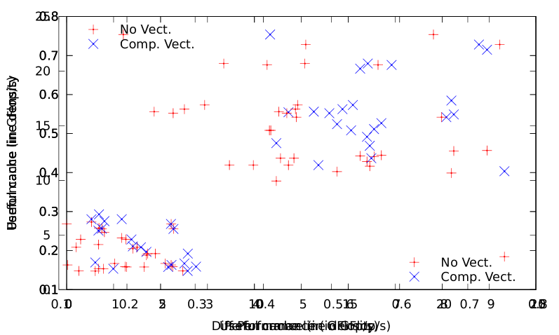
Figure 5: The improvement of -O3 (Comp. Vect.) is linked to cacheline density.

Figure 5 shows the SpMV performance for each matrix with -O1 and -O3 flags as a function of the useful cacheline density (UCLD), a metric we devised for the analysis. For each row, we computed the ratio of the number of nonzeros on that row to the number of elements in the cachelines of the input vector due to that row. Then we took the average of these values to compute UCLD. For instance, if a row has three nonzeros, 0, 19 and 20, the UCLD for that single row would be $\frac{3}{16}$ since there are three nonzeros spread on two cachelines of the input vector (the one storing 0-7 and the one storing 18-25). That is the worst possible value for UCLD is $\frac{1}{8}=0.125$ when only one element of each accessed cacheline is used and the best possible value is $1$ when the nonzeros are packed into well aligned regions of $8$ columns. For each matrix of our data set, there are two points in Figure 5, one giving the performance in -O1 (marked with ‘+’s) and one giving the performance in -O3 (marked with ‘$\times$’s). These two points are horizontally aligned for the same matrix, and the vertical distance between them represents the corresponding improvement on the performance for the matrix. The performance improvement with vectorization, and in particular with vgatherd, is significantly much higher when the UCLD is high. Hence, the maximum performance achieved with vectorial instructions is fairly correlated with UCLD. However, this correlation does not explain what is bounding the computation. The two most common source of performance bound are memory bandwidth and floating point instruction throughput. For Intel Xeon Phi, the peak floating point performance of the architecture is about 1TFlop/s in double precision. Clearly, that is not the bottleneck for our experiments.

4.2 Bandwidth considerations

The nonzeros in the matrix need to be transferred to the core before being processed. Assuming the access to the vectors do not incur any memory transfer, and since each nonzero takes 12 bytes (8 for the value and 4 for the column index) and incurs two floating point operations (multiplication and sum), the flop-to-byte ratio of SpMV is $\frac{2}{12}=\frac{1}{6}$. For our micro benchmarks, we saw that the sustained memory bandwidth is about 180GB/s, which indicates a maximum performance for the SpMV kernel of 30GFlop/s.

Assuming only 12 bytes per nonzero need to be transfered to the core gives only a naive bandwidth for SpMV: both vectors and the row indices also need to be transferred. For an $n\times n$ matrix with $\tau$ nonzeros, the actual minimum amount of memory that need to be transferred in both ways is $2\times n\times 8+(n+1)\times 4+\tau\times(8+4)=4+20\times n+12\times\tau$. If the density of the matrix is high $12\tau$ will dominate the equation, but for sparser matrices, $20n$ should not be ignored. The application bandwidth, which tries to take both terms into account, is a common alternative cross-architecture measure of performance on SpMV.

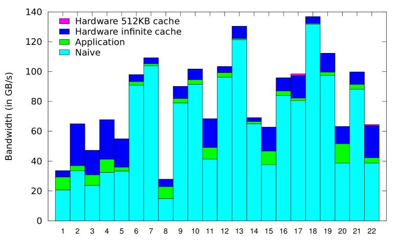
Figure 6: Bandwidth achieved on SpMV with different assumptions.

Figure 6 shows the bandwidth achieved in our experiments. It shows both naive and actual application bandwidths. Clearly, the naive approach ignores a significant portion of the data for some matrices. The application bandwidth obtained ranges from 22GB/s to 132GB/s. Most matrices have an application bandwidth below 100GB/s.

The application bandwidth is computed assuming that every single byte of the problem is transfered exactly once. This assumption is (mostly) true for the matrix and the output vector. However, it does not hold for the input vector for two reasons: first, it is unlikely that each element of the input vector will be used by the threads of a single core, some element will be transferred to multiple cores. Furthermore, the cache of a Xeon Phi core is only 512kB. The input vector does not fit in the cache for most matrices and some matrix elements may need to be transfered multiple times to the same core. We analytically computed the number of cachelines accessed by each core assuming that chunks of 64 rows are distributed in a round-robin fashion (a reasonable approximation of the dynamic scheduling policy). We performed the analysis with an infinite cache and with a 512kB cache. We computed the effective memory bandwidth of SpMV under both assumptions and display them as the top two stacks of the bars in Figure 6. Three observations are striking: first, the difference between the application bandwidth and estimated actual bandwidth is greater than 10GB/s on 10 instances and more than 20GB/s on three of them. The highest difference is seen on 2cubes_sphere (#2) where the amount of data transferred is 1.7 times larger than the application bandwidth. Second, there is no difference between the assumed infinite cache and 512kB cache bandwidth. There is only a visible difference in only two instances: F1 (#17) and cage14 (#22). That is, no cache thrashing occurs. Finally, even when we take the actual memory transfers into account, the obtained bandwidth is still way below the architecture peak bandwidth.

To understand the bottleneck of this application in a better way, we present the application bandwidth of two of the instances for various number of cores and threads per core in Figure 7. We selected these two instances because they seem to be representative for all the matrices. Most of the instances have a profile similar to the one presented in Figure 7(a): there is a significant difference between the performance achieved with 1, 2, 3, and 4 threads. Only 5 matrices, crankseg_2 (#13), pdbHYS (#7), webbase-1M (#8), nd24k (#18), and torso1 (#14), have a profile similar to Figure 7(b): there is barely no difference between the performance achieved with 3 and 4 threads.

Having that many matrices which show a significant difference between 3 and 4 thread/core performance indicates that there is no saturation either in the instruction pipeline or in the memory subsystem bandwidth. Most likely these instances are bounded by the latency of the memory accesses. As mentioned above, SpMV perform equally well for only 5 instances with 3 and 4 threads per core. These instances are certainly bounded by an on-core bottleneck: either the core peak memory bandwidth or the instruction pipeline is full. Three of the instances, crankseg_2, pdbHYS, and nd24k, achieves an application bandwidth over 100GB/s and they are certainly memory bandwidth bound. However two of them, webbase-1M and torso1, reach a bandwidth lesser than 80GB/s.

In both figures, the performance obtained when using 61 cores and 4 threads per core is significantly lower. We believe that using all the threads available in the system hinders some system operations. However, it is strange that this effect was not visible in the bandwidth experiments we conducted in Section 2.1 and 2.2.

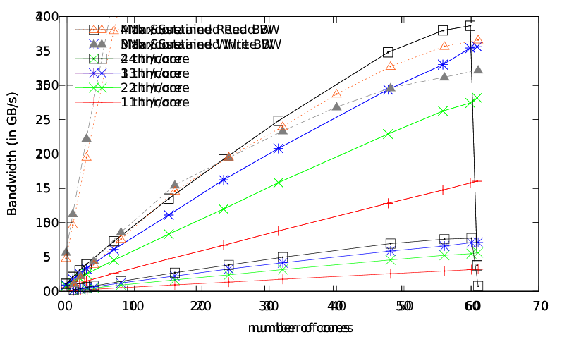
(a) pre2

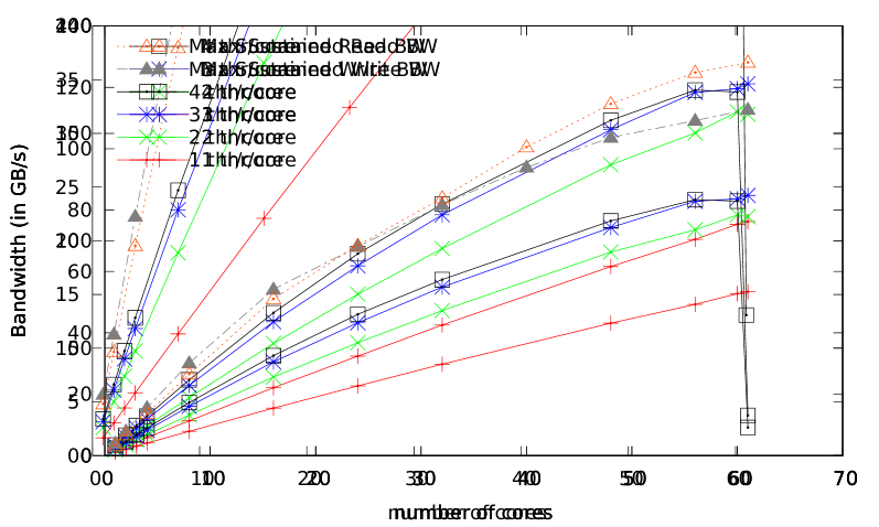
(b) crankseg_2

Figure 7: Strong scaling of application bandwidth for two instances (scheduled with dynamic,64).

4.3 A First summary

We summarize what we learned on SpMV with Intel Xeon Phi: maximizing the usefulness of the vgatherd instruction is the key to optimize the performance: matrices with nonzeros on a row within the same cacheline (within the same 8-column block in double precision) will get a higher performance. This is similar to coalesced memory accesses which is crucial for a good performance while using GPUs.

The difference between the application bandwidth and actual used bandwidth can be high because the same parts of the input vector can be accessed by different cores. Today, cutting edge processors usually have 4-8 cores sharing an L3 cache. However, the Intel Xeon Phi coprocessor has 61 of them, and hence 61 physically different caches. Thus, an improperly structured sparse matrix could require the same part of the input vector to be transferred 61 times. This issue is similar to the problem of input vector distribution in distributed memory SpMV. Moreover, despite the L2 cache of each core is small by today’s standards, we could not observe a cache thrashing during our experiments. At last, for most instances, the SpMV kernel appears to be memory latency bound rather than memory bandwidth bound.

4.4 Effect of matrix ordering

A widely-used approach to improve the performance of the SpMV operation is ordering the rows/columns of the input matrix to make it more suitable for the kernel. Permuting a set of row and columns is a technique used in sparse linear algebra for multiple purposes: improving numerical stability, preconditioning the matrix to reduce the number of iteration and improving performance. Here, we employ the MATLAB implementation of the reverse Cuthill-McKee algorithm (RCM) [5]. RCM has been widely used for minimizing the maximum distance between the nonzeros and the diagonal of the matrix, i.e., the bandwidth of the matrix. It uses a BFS-like vertex/row order w.r.t. the corresponding graph of the matrix and tries to group the nonzeros in a region around the diagonal leaving the area away from the diagonal completely empty. We expect that such a densification of the nonzeros can improve both the UCLD of the matrix and reduce the number of times the vector needed to be transfered from the main memory to the core caches. The results are presented in Figure 8. The improvements in performance, useful cacheline density, and vector access are given so that a positive value is an improvement and a negative value is a degradation. The last metric, Vector Access, represent the expected number of times the input vector needs to be transferred from the memory.

(a) Performance

(b) UCLD

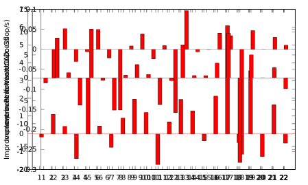
(c) Vector Access

Figure 8: Differences on the performance and metrics when using RCM ordering. A positive value implies an improvement.

The performance improvements are given on Figure 8(a). Matrix F1 (#17) obtains the most absolute improvement which is almost 6GFlop/s. For only 4 matrices, we observe an improvement higher than 2GFlop/s. For most of the matrices, less than 2GFlop/s improvements in the performance are observed, and for 8 matrices, we observe a degradation. For 6 of these matrices, shallow_water1 (#1), mac_econ (#4), pdb1HYS (#7), pre2 (#11), nd24k (#18), and cage14 (#22), an increase can also be observed on the number of times the input vector is transferred. Hence, RCM made these matrices less friendly for the architecture and Vector Access is indeed a crucial and correlated metric for the performance of SpMV on Xeon Phi.

4.5 Effect of register blocking

One of the limitations in the original SpMV implementation is that only a single nonzero is processed at a time. The idea of register blocking is to process all the nonzeros within a region at once. The region should be small enough that the data associated with it can be stored in the registers so as to minimize memory accesses [7]. To implement register blocking, we regularly partitioned $\mathbf{A}$ to blocks of size $a\times b$. If $\mathbf{A}$ has a nonzero within a region the corresponding block is represented as dense (explicitly including the zeros). Hence, the matrix reduces to a list of non-empty blocks and we represent this list via CRS. Since the Xeon Phi architecture has a natural alignment on 512 bits, we chose a block dimension ($a$ or $b$) to be $8$ (8 doubles takes 512 bits). The other dimension varies from 1 to 8. Each dense block can be represented using either a row-major order or a column-major order, depending which dimension is of size 8. When $8\times 8$ are used, experiments show that there is no significant difference between the two schemes.

To perform the multiplication, each block is loaded (or streamed) into the registers in packs of 8 values (zeros and nonzeros) allowing the multiplication to be performed using Fused Multiply-Add operations. Register blocking helps reducing the number of operations needed to process nonzeros inside a block. Furthermore, it can also reduce the size of the matrix: if the matrix has $64$ nonzeros in a dense $8\times 8$ region it would take $768$ bytes in memory with CRS ($64\times 8$ bytes for the value and $64\times 4$ bytes for the offset). With register blocking that region is represented in only 516 bytes since only a single offset is required.

Configuration	8x8	8x4	8x2	8x1	4x8	2x8	1x8
Relative performance	.53	.67	.78	.92	.65	.67	.64
# instances improved	0	2	5	8	2	1	1

Table 2: Performance of register-blocking-based implementation relative to the one without register blocking. The second row presents the geometric means of the relative performance of 22 instances: the ratio of Gflop/s obtained with register blocking to that of the original implementation.

The results obtained with register blocking are summarized in Table 2. We omit the matrix transformation times and only use the timings of matrix multiplications. Overall, we could not observe an improvement. Partitioning with $8\times 1$ blocks is the best scheme and improved performance on 8 instances compared to the original implementation. When register blocking improved performance it was never by more than $25\%$. On average, none of the block sizes helps.

When large blocks are used, the kernel is memory bound (the effective hardware memory bandwidth reaches over 160GB/s in many matrices with only 3 threads per core). However the average relative performance is worse since the matrices have low locality. In $8\times 8$ configuration, less than $35\%$ of the stored values are nonzeros for most of the matrices. That is less than $\frac{23}{64}$ of the transferred memory is useful and too much memory is wasted. According to our experiments, register blocking only saves memory if 70% of the values in the blocks are nonzeros. Unfortunately, none of the matrices respect that condition with $8\times 8$ blocks. However, when the blocks are smaller, the density increases and this explains the increase in relative performance. 10 matrices have more than 50% density at size $8\times 1$ (and 2 have more than 70% density).

Our experiments show that register blocking with dense block storage is not very promising for SpMV on Intel Xeon Phi. Other variants can be still useful: a logical and straightforward solution is storing the the blocks via a sparse storage scheme and generate the dense representation on-the-fly. A 64bit bitmap value would be sufficient to represent the nonzero pattern in a block [3]. Such representations would improve memory usage and increase the relative performance. However, they may not be sufficient to surpass the original implementation two reasons: if the matrices are really sparse any form of register blocking will provide only a little improvement. Besides, register blocking does not change the access pattern to the input vector whose accesses are the one inducing the latency in the kernel.

5 SpMM on Intel Xeon Phi

The flop-to-byte ratio of SpMV limits the achievable performance to at most 30GFlop/s. One simple idea to achieve more performance out of the Xeon Phi coprocessor is to increase the flop-to-byte ratio by performing more than one SpMV at a time. In other words, multiplying multiple vectors will allow us to reach a higher performance. Although not all the applications can take the advantage of the multiple vector multiplication at a time, some applications such as graph based recommendation systems [10] or eigensolvers (by the use of the LOBPCG algorithm) [19] can. Multiplying several vectors by the same matrix boils down to multiplying a sparse matrix by a dense matrix, which we refer to as SpMM. All the statements above are also valid for existing cutting-edge processors and accelerators. However, with its large SIMD registers, Xeon Phi is expected to perform significantly better.

In our SpMM implementation for the operation $\mathbf{Y}\leftarrow\mathbf{A}\mathbf{X}$, the dense $m\times k$ input matrix $\mathbf{X}$ is encoded in row-major, so each row is contiguous in memory. To process a row $\mathbf{A}_{i*}$ of the sparse matrix, a temporary array of size $k$ is first initialized to zero. Then for each nonzero in $\mathbf{A}_{i*}$, a row $\mathbf{X}_{j*}$ is streamed to be multiplied by the nonzero and the result is accumulated into the temporary array. We developed three variants of that algorithm for Xeon Phi: the first variant is a generic code which relies on compiler vectorization. The second is tuned for values of $k$ which are multiple of $8$. This code is manually vectorized to load the row of the vector by blocks of 8 doubles in a SIMD register and perform the multiplication and accumulation using Fused Multiply-Add. The temporary values are kept in registers by taking the advantage of the large number of SIMD registers available on Xeon Phi. In the third variant, we use Non-Globally Ordered write instructions with No-Read hint (NRNGO) and that proved to be fastest in our bandwidth experiments.

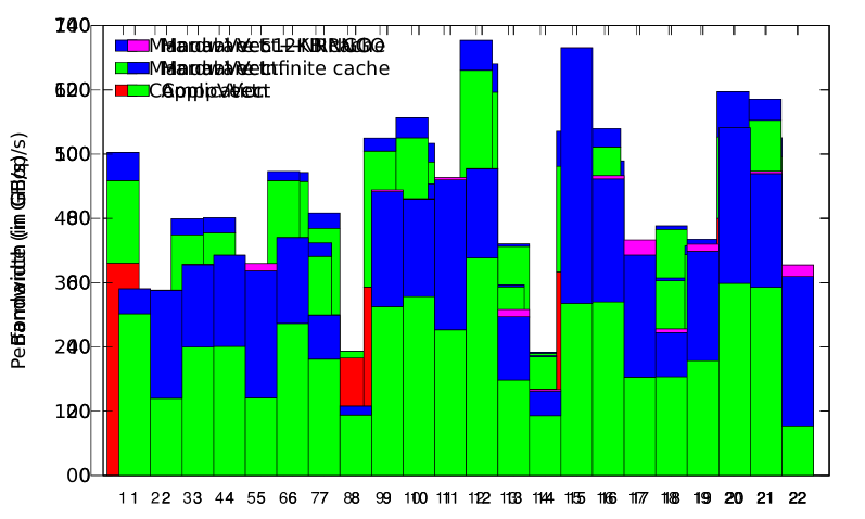
(a) Comparison of three SpMM variants

(b) Bandwidth of Manual Vect. + NRNGO

Figure 9: Performance of SpMM with $k=16$. NRNGO is the variant with No-Read hint and Non-Globally ordering.

We experimented with $k=16$ and present the results in Figure 9. In many instances, manual vectorization doubles the performance allowing to reach more than 60GFlop/s in 11 instances. The use of the NRNGO write instructions provides significant performance improvements. The achieved performance peaks on the matrix pwtk matrix at 128GFlop/s. Figure 9(b) shows the bandwidth achieved by the best implementation. The application bandwidth surpasses 60GB/s in only $1$ instance. The size of the data is computed as $8\times m\times k+8\times n\times k+(n+1)\times 4+\tau\times(8+4)$. However, since there are 16 input vectors, the overhead induced by transferring the values in $\mathbf{X}$ to multiple cores is much higher when the amount of data transfers are taken into account while computing the application bandwidth. Once again, the impact of having a finite cache is only very small. Hence, similar to SpMV, the cache size is not the problem for Xeon Phi, but having 61 different caches can be a problem for some applications.

6 Against other architectures

We compare the sparse matrix multiplication performance of Xeon Phi with 4 other architectures including 2 GPU configurations and 2 CPU configurations. We used two CUDA-enabled cards from NVIDIA. The NVIDIA Tesla C2050 is equipped with 448 CUDA Cores clocked 1.15GHz and 2.6GB of memory clocked at 1.5GHz (ECC on). This machine uses CUDA driver and CUDA runtime 4.2. The Tesla K20 comes with 2,496 CUDA Cores clocked at 0.71GHz and 4.8GB of memory clocked at 2.6GHz (ECC on). This machine uses CUDA driver and CUDA runtime 5.0. For both GPU configurations, we use the CuSparse library as implementation. We also use two Intel CPU systems: the first one is a dual Intel Xeon X5680 configuration, which we call as Westmere. Each processor is equipped with $6$ cores clocked at $3.33$Ghz and hyperthreading is disabled. Each processor is equipped with a shared $12$MB L3 cache, and each core has a local $256$kB L2 cache. The second configuration is a dual Intel Xeon E5-2670, which we denote with Sandy. Each processor is equipped with 8 cores clocked at 2.6GHz and hyperthreading is enabled. Each processor is equipped with a shared $20$MB L3 cache, and each core has a local $256$kB L2 cache. All the codes for both CPU architectures are compiled with the icc 13.0 with -O3 optimization flag. All kernels are implemented with OpenMP. For the performance and stability, all runs are performed with thread pinning using KMP_AFFINITY. The implementation used is the same as the one used on Xeon Phi except the vector optimizations in SpMM where the instruction sets differ.

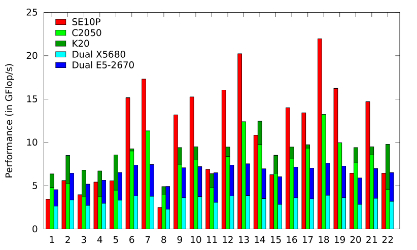
(a) SpMV

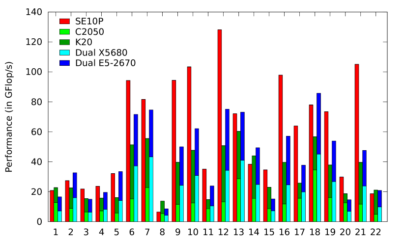
(b) SpMM

Figure 10: Architectural comparison between a Intel Xeon Phi coprocessor (Pre-release SE10P), two NVIDIA GPUs (C2050 and K20) and two dual CPU architectures (Intel Xeon X5680 and Intel Xeon E5-2670).

Results of the experiments are presented in Figure 10. Since we have two GPU and two CPU architectures where one is expected to be better than the other, we present them as stacked bar charts: K20 on top of C2050 and Sandy on top of Westmere. Figure 10(a) shows the SpMV results: Sandy appears to be roughly twice faster than Westmere. It reaches a performance between 4.5 and 7.6GFlop/s and achieves the highest performance for one instance. For GPU architectures, the K20 card is typically faster than the C2050 card. It performs better for 18 of the 22 instances. It obtains between 4.9 and 13.2GFlop/s and the highest performance on 9 of the instances. Xeon Phi reaches the highest performance on 12 of the instances and it is the only architecture which can obtain more than 15GFlop/s. Furthermore, it does it for 7 of the instances.

Figure 10(b) shows the SpMM results: Sandy gets twice the performance of the Westmere, which is similar to their relative SpMV performances. The K20 GPU is often more than twice faster than C2050, which is much better compared with their relative performances in SpMV. The Xeon Phi coprocessor gets the best performance in 14 instances where this number is $5$ and $3$ for the CPU and GPU configurations, respectively. Intel Xeon Phi is the only architecture which achieves more than 100GFlop/s. Furthermore, it reaches more than 60GFlop/s on 9 instances. The CPU configurations reach more than 60GFlop/s on 6 instances while the GPU configurations never achieve that performance.

7 Conclusion and Future Work

In this work, we analyze the performance of Intel Xeon Phi coprocessor on SpMV and SpMM. These sparse algebra kernels have been used in many important applications. To the best of our knowledge, the analysis gives the first absolute performance results of Intel Xeon Phi.

We showed that the sparse matrix kernels we investigated are latency bound. Our experiments suggested that having a relatively small 512kB L2 cache per core is not a problem for Intel Xeon Phi. However, having 61 cores brings increase/decrease in the usefulness of existing optimization approaches in the literature. Although it is usually a desired property, having a large number of cores can have a negative impact on the performance especially if the input data is large and it is required to be transferred to multiple caches. This increase the importance of matrix storage schemes, intra-core locality, and data partitioning among cores. As a future work, we are planning to investigate such techniques in detail to improve the performance of Xeon Phi.

Overall, the performance of the coprocessor is very promising. When compared with cutting-edge processors and accelerators, its SpMV, and especially SpMM, performance are superior thanks to its wide registers and vectorization capabilities. We believe that Xeon Phi will gain more interest in HPC community in the near future.

References

- [1] N. Bell and M. Garland. Implementing sparse matrix-vector multiplication on throughput-oriented processors. In Proc. High Performance Computing Networking, Storage and Analysis, SC ’09, pages 18:1–18:11, 2009.
- [2] A. Buluç, J. T. Fineman, M. Frigo, J. R. Gilbert, and C. E. Leiserson. Parallel sparse matrix-vector and matrix-transpose-vector multiplication using compressed sparse blocks. In Proc. SPAA ’09, pages 233–244, 2009.
- [3] A. Buluç, S. Williams, L. Oliker, and J. Demmel. Reduced-bandwidth multithreaded algorithms for sparse matrix-vector multiplication. In Proc. IPDPS, 2011.
- [4] T. Cramer, D. Schmidl, M. Klemm, and D. an Mey. Openmp programming on intel xeon phi coprocessors: An early performance comparison. In Proceedings of the Many-core Applications Research Community (MARC) Symposium at RWTH Aachen University, Nov. 2012.
- [5] E. Cuthill and J. McKee. Reducing the bandwidth of sparse symmetric matrices. In Proc. ACM national conference, pages 157–172, 1969.
- [6] J. Eisenlor, D. E. Hudak, K. Tomko, and T. C. Prince. Dense linear algebra factorization in OpenMP and Cilk Plus on Intel MIC: Development experiences and performance analysis. In TACC-Intel Highly Parallel Computing Symp., 2012.
- [7] E.-J. Im and K. A. Yelick. Optimizing sparse matrix computations for register reuse in sparsity. In Proc. of ICCS, pages 127–136, 2001.
- [8] A. Jain. pOSKI: An extensible autotuning framework to perform optimized spmvs on multicore architecture. Master’s thesis, UC Berkeley, 2008.
- [9] M. Krotkiewski and M. Dabrowski. Parallel symmetric sparse matrix-vector product on scalar multi-core CPUs. Parallel Comput., 36(4):181–198, Apr. 2010.
- [10] O. Küçüktunç, K. Kaya, E. Saule, and Ü. V. Çatalyürek. Fast recommendation on bibliographic networks. In Proc. ASONAM’12, Aug 2012.
- [11] J. Mellor-Crummey and J. Garvin. Optimizing sparse matrix-vector product computations using unroll and jam. Int. J. High Perform. Comput. Appl., 18(2), May 2004.
- [12] R. Nishtala, R. W. Vuduc, J. W. Demmel, and K. A. Yelick. When cache blocking of sparse matrix vector multiply works and why. Appl. Algebra Eng., Commun. Comput., 18(3):297–311, May 2007.
- [13] S. Potluri, K. Tomko, D. Bureddy, and D. K. Panda. Intra-MIC MPI communication using MVAPICH2: Early experience. In TACC-Intel Highly Parallel Computing Symp., 2012.
- [14] Y. Saad. Sparskit: a basic tool kit for sparse matrix computations - version 2, 1994.
- [15] E. Saule and Ü. V. Çatalyürek. An early evaluation of the scalability of graph algorithms on the Intel MIC architecture. In IPDPS Workshop MTAAP, 2012.
- [16] K. Stock, L.-N. Pouchet, and P. Sadayappan. Automatic transformations for effective parallel execution on intel many integrated core. In TACC-Intel Highly Parallel Computing Symp., 2012.
- [17] R. Vuduc, J. Demmel, , and K. Yelic. OSKI: A library of automatically tuned sparse matrix kernels. In Proc. SciDAC 2005, J. of Physics: Conference Series, 2005.
- [18] S. Williams, L. Oliker, R. Vuduc, J. Shalf, K. Yelick, and J. Demmel. Optimization of sparse matrix-vector multiplication on emerging multicore platforms. In Proc. SC ’07, pages 38:1–38:12, 2007.
- [19] Z. Zhou, E. Saule, H. M. Aktulga, C. Yang, E. G. Ng, P. Maris, J. P. Vary, and Ü. V. Çatalyürek. An out-of-core eigensolver on SSD-equipped clusters. In Proc. of IEEE Cluster, Sep 2012.